Simulation of air shower image in fluorescence light based on energy deposits derived from CORSIKA

Abstract

Spatial distributions of energy deposited by an extensive air shower in the atmosphere through ionization, as obtained from the CORSIKA simulation program, are used to find the fluorescence light distribution in the optical image of the shower. The shower image derived in this way is somewhat smaller than that obtained from the NKG lateral distribution of particles in the shower. The size of the image shows a small dependence on the primary particle type.

1 Introduction

The fluorescence method of extensive air shower detection is based on recording light emitted by air molecules excited by charged particles of the shower. For very high energies of the primary particle, enough fluorescence light is produced by the large number of secondaries in the cascading process so that the shower can be recorded from a distance of many kilometers by an appropriate optical detector system [1, 2]. As the amount of fluorescence light is closely correlated to the particle content of a shower, it provides a calorimetric measure of the primary energy.

The particles in an air shower are strongly collimated around the shower axis. Most of them are spread at distances smaller than several tens of meters from the axis, so that when viewed from a large distance, the shower resembles a luminous point on the sky. Therefore, a one-dimensional approximation of the shower as being a point source might be adequate in many cases regarding the shower reconstruction. For more detailed studies, however, the spatial spread of particles in the shower has to be taken into account. This is especially important for nearby showers, where the shower image, i.e. the angular distribution of light recorded by a fluorescence detector (FD), may be larger than the detector resolution.

The image of a shower has been studied in Ref. [3], where it was shown that for a disk-like distribution of the light emitted around the shower axis, the shower image has a circular shape, even when viewed perpendicular to the shower axis. Analytical studies including lateral particle distributions parameterized by the Nishimura-Kamata-Greisen (NKG) function or estimates based on average particle distributions taken from CORSIKA [4] were discussed in Ref. [5] and Ref. [6], respectively.

In this paper, detailed Monte Carlo simulations of the shower image based on the spatial energy deposit distributions of individual showers are performed. By using the energy deposit of the shower particles as calculated by CORSIKA [7], the previous simplified assumption of a constant fluorescence yield per particle is avoided. Assuming a proportionality between the fluorescence yield and ionization density, the light emitted by each segment of the shower is determined. A concept is developed to treat the shower as a three-dimensional object, additionally taking into account the time information on photons arriving at the FD. In contrast to previous analytical studies, shower fluctuations as predicted by the shower simulation code are preserved and studied. Propagation of the light towards the detector, including light attenuation and scattering in the atmosphere is simulated, so that the photon flux at the detector is calculated. The resulting distribution of photons arriving simultaneously at the detector, i.e. the shower image, is compared to results obtained by using the NKG approximation of particle distribution in the shower. The comparison is performed for different shower energies and different primary particles. In particular, it is checked whether the shower width depends on the primary particle type.

The plan of the paper is the following: definition of the shower width and algorithms of fluorescence light production are described in Section 2. In Section 3 the size of shower image in the NKG and CORSIKA approaches is calculated and its dependence on primary energy, zenith angle and primary particle is discussed. Conclusions are given in Section 4.

2 Simulations

2.1 Shower width and shape function

Given an optical imaging system for recording the light emitted by a shower, the shower width is defined as the minimum angular diameter $\alpha$ of the image spot containing a certain fraction $F(\alpha)$ of the total light recorded by the FD. The image is considered to be recorded instantaneously, i.e. with an integration time such that the corresponding angular shower movement is well below the angular resolution of the detector.

Four main components of light contribution can be distinguished: (i) fluorescence light, with isotropic emission; (ii) direct Cherenkov radiation, emitted primarily in the forward direction; (iii) Rayleigh-scattered Cherenkov light; (iv) Mie-scattered Cherenkov light. The relative contributions of these components depend on the geometry of the shower with respect to the detector [8], but in most cases the fluorescence light dominates the recorded signal. Assuming only minor effects on the shower width by absorption and scattering processes during the fluorescence light propagation from the shower to the detector, the light fraction $F(\alpha)$ is mainly determined by the corresponding light fraction $F(r)$ emitted around the shower axis

$$F(r)=\int_{0}^{r}f(r)2\pi rdr~{},$$ (1)

where $f(r)$ is the (normalized) lateral distribution of fluorescence light emitted. The main task is therefore to derive $f(r)$, which is also referred to as the shape function, since the brightness distribution of the shower image depends on the shape of $f(r)$. The shape functions in different methods of evaluating fluorescence light production described in the following, i.e. in the NKG and CORSIKA approach, and for different primary particle types in the CORSIKA approach will be compared.

Photon propagation towards the detector is simulated based on the Hybrid_fadc simulation software [9], including Rayleigh scattering on air molecules and Mie scattering on aerosols. The final shower image is constructed by recording the photons that arrive simultaneously at the detector [5]. These photons that form an instantaneous image of the shower, originate from a range of shower development stages. Thus, for a precise description of the shower image, we need to take into account also the geometrical time delays of the photons coming from these stages, as will be discussed later.

Since this work is intended as a general study, the resulting photon distribution after light propagation is assumed to be recorded by an ideal detector. Possible effects of specific detector conditions such as spatial resolution or trigger thresholds will also be commented on, however. Investigations specific to the fluorescence detectors of the Pierre Auger Observatory are described in Ref. [10]

2.2 Fluorescence light production

As the shower develops in the atmosphere, it dissipates most of its energy by exciting and ionizing air molecules along its path. From de-excitation, UV radiation is emitted with a spectrum peaked between 300 and 400 nm (three major lines at 337.1 nm, 357.7 nm, 391.4 nm). Measurements have shown that the variation of the fluorescence yield $n_{\gamma,0}$, i.e. the number of photons emitted per unit length along a charged particle track, as a function of altitude is quite small for electrons of constant energy. For example, the measured fluorescence yield of an 80 MeV electron varies by less than 12% around an average value of 4.8 photons/m over an effective altitude range of 20 km in the atmosphere [11]. This motivates to some extent the use of a constant, average fluorescence yield per shower particle, as will be described in the NKG approach (section 2.2.1).

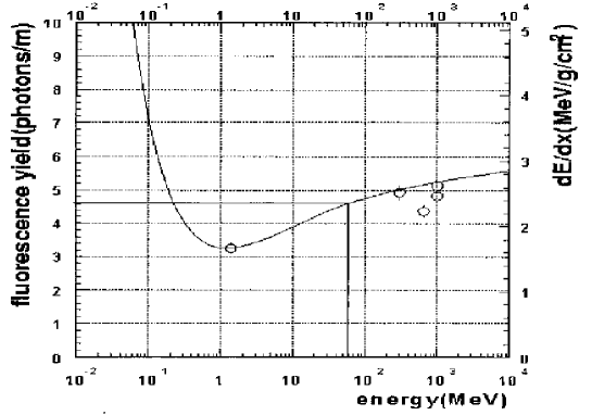
Figure 1: Energy dependence of nitrogen fluorescence between 300 and 400 nm in dry air at the pressure 760 mm Hg. The scale of fluorescence yield is adjusted so that the 1.4 MeV point lies on the $dE/dX$ curve (taken from Ref. [11]).

On the other hand, since the fluorescence light is induced by ionizing and exciting the molecules of the ambient air, the fluorescence yield is expected to depend on the ionization density along a charged particle track [11, 12, 13]. Most shower particles contributing to the energy deposit in air have kinetic energies from sub-MeV up to several hundred MeV [7] which is in the energy range of considerable dependence of ionization density on particle energy. As an example, a measurement of the air fluorescence yield [11] between 300 and 400 nm at pressure 760 mm Hg is shown in Figure 1. The solid line represents the electron energy loss $dE/dX$ as a function of the electron energy. The minimum of this curve corresponds to 1.4 MeV electrons with energy loss $\langle dE/dX\rangle|_{1.4MeV}=1.668$ MeV/gcm^-2 and fluorescence yield $n_{\gamma,0}=3.25$ photons per meter. We note that $dE/dX$ increases by about $50\%$ for energies from 1.0 MeV to 100 MeV, so the energy spectrum of electrons in a shower and its variations with atmospheric depth should be taken into account for an accurate determination of the fluorescence emission of the shower. Therefore to obtain a more realistic simulation of the spatial distribution of light production, the distribution of the energy deposit in the shower is used in the CORSIKA approach (section 2.2.2), where additionally the temperature and density dependence of the fluorescence yield is taken into account.

2.2.1 NKG approach

In the usual treatment that was also used in a previous study of the shower image [5], the fluorescence light emitted by a shower is calculated from [2]:

$$\frac{d^{2}N_{\gamma}}{dld\Omega}\simeq\frac{n_{\gamma,0}N_{e}}{4\pi}{\hskip 14.22636pt}\left[\frac{\mbox{photon}}{\mbox{sr }\mbox{m}}\right]$$ (2)

where $n_{\gamma,0}$ is a constant value of total fluorescence yield. The total number of particles $N_{e}=\int\rho_{N}(X,r)2\pi rdr$ is given by the Gaisser-Hillas function [1]

$$N_{e}(X)=N_{max}\left(\frac{X-X_{0}}{X_{max}-X_{0}}\right)^{(X_{max}-X_{0})/\lambda}\exp{((X_{max}-X)/\lambda)}$$ (3)

where $N_{max}$ is the number of particles at shower maximum given by [14]

$$N_{max}=0.7597\left(\frac{E_{0}[GeV]}{10^{9}}\right)^{1.010}*10^{9}$$ (4)

and $\rho_{N}(X,r)$ is density of electrons in the shower given by the Nishimura-Kamata-Greisen (NKG) formula [15]

$$\rho_{N}(X,r)=\frac{N_{e}(X)}{r_{M}^{2}}(\frac{r}{r_{M}})^{s-2}(1+\frac{r}{r_{M}})^{(s-4.5)}\frac{\Gamma(4.5-s)}{2\pi\Gamma(s)\Gamma(4.5-2s)},$$ (5)

$X$ is the atmospheric slant depth, $X_{0}$ the depth of first interaction, $X_{max}$ the depth of shower maximum, $\lambda$ the hadronic interaction length in air (commonly fixed to a value of $70$ g/cm²), $s$ the shower age parameter ($s=1$ at shower maximum) and $r_{M}$ the Molière radius.

The Molière radius is a natural transverse scale set by multiple scattering, and it determines the lateral spread of the shower. Since the electron radiation length (the cascade unit) in air depends on temperature and pressure, the Molière radius varies along the shower path. The distribution of particles in a shower at a given depth depends on the history of the changes of $r_{M}$ along the shower path rather than on the local $r_{M}$ value at this depth. To take this into account, one uses the $r_{M}$ value calculated at $2$ cascade units above the current depth [16]:

$$r_{M}[\mbox{m}]=272.5\frac{T[\mbox{K}](\frac{P[\mbox{mb}]-73.94\cos\theta}{P[\mbox{mb}]})^{1./5.25588}}{P[\mbox{mb}]-73.94\cos\theta}.$$ (6)

In the NKG approach we keep a constant value of fluorescence yield $n_{\gamma,0}=4.02$ photons per meter, as used by the HiRes group [2]. The spatial distribution of emitted light is therefore also given by the NKG formula, and the shape function follows from Eq. (5) as $f_{\rm NKG}(r)=\rho_{N}(X,r)/N_{e}(X)$. The fluorescence light fraction $F_{\rm NKG}(r)$ using equation (1) can then be determined analytically by the normalized incomplete beta function,

$$F_{\rm NKG}(r)=I_{x}(a,b)=\frac{1}{B(a,b)}\int_{0}^{x}u^{a-1}(1-u)^{b-1}du$$ (7)

where $x=1/(1+r_{M}/r)$, $a=s$, $b=4.5-2s$ and $B(a,b)$ is Euler’s beta function. Using the series expansion of $I_{x}(a,b)$, [17] the fluorescence light fraction can be given by

$$F_{\rm NKG}(r)=\left(\frac{1}{1+\frac{r_{M}}{r}}\right)^{4.5-s}\frac{1}{sB(s,4.5-2s)}\\ \left(1+\sum_{n=0}^{\infty}\frac{B(s+1,n+1)}{B(4.5-s,n+1)}\left(\frac{1}{1+\frac{r_{M}}{r}}\right)^{n+1}\right)$$ (8)

For $s=1$ formula (8) reduces to

$$F_{\rm NKG}(r)=1-\left(1+\frac{r}{r_{M}}\right)^{-2.5}.$$ (9)

Inverting the above equation and taking into account the distance from the detector to the shower ($R$) we can find the angular size $\alpha_{{\rm NKG}}$ that corresponds to a certain fraction of the total fluorescence light signal:

$$\alpha_{{\rm NKG}}=2\arctan\left(\frac{r}{R}\right)=2\arctan(\frac{r_{M}}{R}((1-F_{\rm NKG}(r))^{-0.4}-1)).$$ (10)

2.2.2 CORSIKA approach based on energy deposit

In contrast to the NKG approach, the fluorescence light production in the CORSIKA approach is connected to the local energy release of the shower particles in the air; additionally, a dependence of the yield on the local atmospheric conditions is taken into account:

$$n_{\gamma,0}(\lambda)=\epsilon_{\lambda}(P,T)\frac{\lambda}{hc}\frac{dE}{dX}\rho_{air}{\hskip 14.22636pt}\left[\frac{\mbox{photon}}{\mbox{m}}\right]$$ (11)

where $\epsilon_{\lambda}(P,T)$ is the fluorescence efficiency; $\rho_{air}$, $P$ and $T$ are density, pressure and temperature of air, respectively; $\lambda$ is the photon wavelength, $c$ is speed of light and $h$ is the Planck constant.

In the CORSIKA shower simulation program, the energy loss $dE/dX$ of the shower particles is calculated in detail, taking into account also the contribution of particles below the simulation energy threshold [7]. We extended the code to obtain a spatial distribution of the energy deposit. This offers the possibility to construct a shower simulation chain which allows the comparison of quantities very close to the measured ones, e.g. photon flux or distribution of light received at the detector or even per pixel as a function of time. In particular, shower-to-shower fluctuations generated by CORSIKA are preserved in this way.

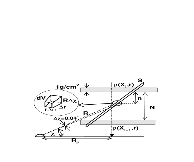
Figure 2: Geometry of an EAS as seen by the fluorescence detector. Photons which arrive simultaneously to the FD originate from surface S. See text for more details.

The adopted air shower simulation part of the simulation chain is illustrated in Figure 2. A two-dimensional energy deposit distribution around the shower axis is stored in histograms during the simulation process for different atmospheric depths. By interpolation between the different atmospheric levels, a complete description of the spatial energy deposit distribution of the shower, taking into account also the geometrical time delays, is achieved. More specifically, the lateral energy deposit $\rho_{E}(X_{i},r)$ is calculated for 20 horizontal layers of $\Delta X=1$ g/cm². Each observation level corresponds to a certain vertical atmospheric depth, the first one to $X_{1}=120$ g/cm² and the last one to $X_{20}=870$ g/cm².

The simultaneous photons, which constitute an instantaneous image of the shower, originate from a range of shower development stages [5], from the surface $S$ as shown in Figure 2. These simultaneous photons are defined as those which arrive at the FD during a short time window $\Delta t$. During this $\Delta t$ (corresponding to a small change of the shower position in the sky by $\Delta\chi=0.04^{\circ}$ as chosen in the code) the shower front moves downward along the shower axis by a small distance $R\Delta\chi$. This means that the small element of surface $S$ in polar coordinates corresponds to a small volume $\Delta V=r\Delta\phi\Delta rR\Delta\chi$, where $\Delta\phi$ and $\Delta r$ are steps in the azimuth angle and in the radial direction relative to the shower axis and $R$ is the distance from the FD to the volume $\Delta V$. The volume $\Delta V$ is located between two CORSIKA observation levels $X_{i}$ and $X_{i+1}$. The distance between these two levels is divided into $N$ sublevels, each of them labeled by $n$. Due to the small spacing between the chosen CORSIKA levels, the value of energy deposit within the volume $\Delta V$ at distance $r$ can then be constructed sufficiently well by linear interpolation:

$$\rho_{E}(X_{n},r)=\frac{(N-n)\rho_{E}(X_{i},r)+n\rho_{E}(X_{i+1},r)}{N}.$$ (12)

An additional linear interpolation in radial direction between bins of the CORSIKA output was used to find the density $\rho_{E}(X_{n},r)$ of the energy deposit.

Using the above interpolation, the number of photons $N_{\gamma}$ from the volume $\Delta V$ that are emitted towards the FD can be calculated as:

$$N_{\gamma}=\frac{\rho_{E}(X_{n},r)dS}{\langle dE/dX\rangle|_{1.4MeV}}\sum_{i=1}^{16}\epsilon_{i}g_{i}(\rho,T)\frac{\Delta\chi A}{4\pi R_{p}}$$ (13)

where i runs over 16 wavelength bins, $\epsilon_{i}$ is the fluorescence yield for a 1.4 MeV electron at pressure of 760 mm Hg and temperature of 14^∘ C, $dS$ is a projection of the surface $r\Delta\phi\Delta r$ into surface perpendicular to direction of the shower axis, $\langle dE/dX\rangle|_{1.4MeV}$ is the electron energy loss evaluated at 1.4 MeV, $A$ is the light collecting area of the FD, $R_{p}$ is the shower impact parameter with respect to the FD and $g_{i}(\rho,T)$ is a function describing the dependence of the fluorescence yield on the density $\rho$ and temperature $T$ of the air. Kakimoto et al. [11] provided an analytical formula for $g_{i}(\rho,T)$. For the 391.4 nm fluorescence line (13th bin in formula (13))

$$g_{13}(\rho,T)=\frac{\rho A_{2}}{F_{1}(1+\rho B_{2}\sqrt{T})}$$ (14)

and for the rest of the fluorescence spectrum

$$g_{i}(\rho,T)=\frac{\rho A_{1}}{2.760F_{1}(1+\rho B_{1}\sqrt{T})}$$ (15)

where $\rho$ is in units of g/cm³ and T is in Kelvin. $F_{1}$, $A_{1}$, $A_{2}$, $B_{1}$ and $B_{2}$ are constants and are $1.044\times 10^{-5}$, 0.929 cm²g^-1, 0.574 cm²g^-1, 1850 cm³g^-1K^-1/2, 6500 cm³g^-1K^-1/2, respectively. The value of 2.760 photon/m is the total fluorescence yield outside the 391 nm band.

In the CORSIKA simulations performed for this analysis, electromagnetic interactions are treated by an upgraded version [18] of the EGS4 [19] code. High-energy hadronic interactions are calculated by the QGSJET [20] interaction model. To reduce computing time for the simulation of high-energy events, a thinning algorithm [21] is selected within CORSIKA: Only a subset of the secondary particles that have energies below a specified fraction of the primary energy are tracked in detail. An appropriate weight is attached to each tracked particle to assure energy conservation. The artificial fluctuations introduced by thinning are sufficiently small, when a thinning level of $10^{-6}$ with optimum weight limitation [18, 22, 23] has been chosen. This weight limitation stops thinning in case of large particle weights and includes different weight limits for the electromagnetic component compared to the muonic and hadronic ones.

3 Results

Simulation runs were performed for proton and iron showers for different primary energy $E_{0}$. The depth of first interaction $X_{0}$ in the NKG approximation was chosen according to the average depth $X_{0}$ from CORSIKA, see Table 1. Showers landing at variable core distance $R_{p}=2,3,...,11$ and $12$ km were studied. The results shown in the following refer to the shower maximum, where also the fluorescence emission is largest.

3.1 Shower image in the NKG approach

The shape function of particle density $f_{{\rm NKG}}(r)$ at shower maximum is shown in Figure 3A for vertical and inclined ($\theta=45^{\circ}$) showers with $E_{0}=10$ EeV and $E_{0}=100$ EeV. It can be seen that these shape functions are almost identical. Some differences between vertical and inclined showers are seen only at distances to shower axis larger than $\simeq 50$ m. The differences are due to changes of the Molière radius with altitude: a larger zenith angle of the shower implies a higher position of the shower maximum and in consequence a larger value of the Molière radius. Since the Molière radius determines the lateral spread of particles in the shower, for inclined showers the shape function $f_{{\rm NKG}}(r)$ becomes broader. A similar effect can be observed for showers with the same geometry, but different energies (showers with lower energy have a higher position of the maximum and also a larger Molière radius) but in these cases the differences are much smaller.

In the NKG approach the size of the shower image $\alpha_{{\rm NKG}}$ is connected to the width of the shape function of particle density $f_{{\rm NKG}}(r)$ and can be calculated at shower maximum using Eq. (10) for fixed Molière radius, fraction of fluorescence light $F_{{\rm NKG}}(r)$ and the detector-to-shower distance $R$. The appropriate $F_{{\rm NKG}}(r)$ functions for showers presented in Figure 3A are shown in Figure 3B. It is seen that 90% (67%) of fluorescence light emitted (i.e. of shower particles) are found within distances about 160 m (58 m) around shower axis for vertical showers and about 190 m (70 m) for inclined showers. The corresponding angular width of fluorescence light distributions at the detector, positioned for instance at $R=3.16$ km, in these cases is about 5.7^∘ (2^∘) for vertical showers and 7.0^∘ (2.6^∘) for inclined showers. In Table 2 the sizes of shower image containing 90% and 67% of the signal according to formula (10) are listed. There is about 5% difference in the image spot size of showers with the same zenith angle but different energy, and about 19% between inclined and vertical showers. In Figure 3C the dependence of shower image versus $R$ in the NKG approach is shown. The $90\%$ spot size exceeds $1.5^{\circ}$ for vertical (inclined) showers at distances smaller than 12 km (14.5 km). With typical FD pixel resolution of $1$–$1.5^{\circ}$, the shower image will cover more than one pixel at these distances. For a correct primary energy determination of these events, the fluorescence light in the neighboring pixels has to be taken into account. For example, at $R=3.16$ km the fraction of light outside the circle corresponding to pixel field of view ($1.5^{\circ}$ in diameter) is about 40%, as marked by the vertical dashed line in Figure 3B, but only about 10% if the $R$ increases 4 times (increasing $R$ leads to proportional decreasing of image size). Neglecting this effect would result in a significant underestimation of the reconstructed primary energy, especially for nearby showers. The analysis of Figure 3 and Table 2 leads to the following conclusion: in case of the NKG approximation the size of the shower image is independent of the primary energy for showers at the same development stage and geometry. In other words, the same Molière radius and shower age imply the same shape of $f_{{\rm NKG}}(r)$ function and in consequence lead to the same spot size of the shower image.

In the above estimation of shower image we have neglected the influence of Rayleigh- and Mie-scattered and direct Cherenkov light distribution on the shower image size. To estimate this effect, relative differences between shower images obtained using these additional contributions to the fluorescence flux with respect to fluorescence only are shown in Figure 4. The additional contributions to the fluorescence light increase the image size on average by about 7% (3%) within the image size containing 90% (67%) of light and these changes of shower image size slightly depend on $R$. These changes can be well understood if we take into account the Rayleigh scattering, which is the second dominant component in the total signal for the studied geometry. It is well known that Rayleigh scattering probability is proportional to $(1+\cos^{2}\xi)$, where $\xi$ is the angle between the direction of photon emission and the direction towards the FD. Since $\xi$ increases for a vertical shower with increasing $R$, so the Rayleigh scattering probability and also contribution of Rayleigh-scattered light to the shower image will be smaller. We note from Figure 4 that this contribution depends on the fraction of light considered: it is larger when we study 90% of light than for 67%. This means that in the ”center” of shower image fluorescence dominates, but it is less in the ”tail”. The shower image in the scattered light is therefore larger, although the ”scattered” contribution is small for the considered geometries. In the following we concentrate on the main component, the unscattered fluorescence light.

3.2 Comparison of shower image in the NKG and CORSIKA approaches

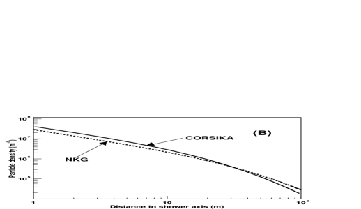
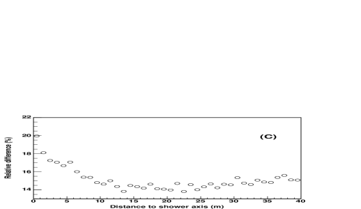
Figure 5: (A) Lateral distributions of energy deposit density in the CORSIKA and NKG approximations, calculated for an average vertical proton shower with energy 10 EeV. (B) Particle density from CORSIKA and derived using NKG function, (C) Relative difference $z$ between average energy loss obtained from the CORSIKA and NKG approaches.

In this section we study the differences between the calculated lateral distributions of energy deposit in the NKG and CORSIKA approaches and their influence on the shower image. We assume that fluorescence emmision dominates the received signal and that the distribution of light emitted by the shower is proportional to the distribution of energy deposit: $f(r)\sim\rho_{E}(X,r)$. For this purpose, in Figure 5A we show the calculated lateral distributions of the energy deposit versus the distances to the shower axis at any point of surface S (see Figure 2). In case of the NKG approximation, the lateral density of energy deposit (dashed line) is calculated using the following formula:

$$\rho_{{\rm NKG}}(X,r)=\langle dE/dX\rangle N_{max}f_{{\rm NKG}}(r)$$ (16)

where $\langle dE/dX\rangle$ is the energy loss of an electron corresponding to a constant value of the average fluorescence yield $n_{\gamma,0}=4.02$ photons per meter.

In case of the CORSIKA approach, the energy deposit density (solid line in Figure 5A) was obtained using the two-dimensional histogram of $dE/dX$. It is seen that the density of energy deposit obtained using CORSIKA histograms becomes larger than NKG at distances to shower axis smaller than 45 m. In the NKG approximation, it is assumed that all particles lose the same amount of energy and that the shape of the lateral distribution of energy deposit has the same (NKG) functional form. Plots in Figures 5B and 5C show that these assumptions are not strictly valid. In Figure 5B we see that the particle density calculated from the NKG formula (dashed line) is different from the particle density from CORSIKA (solid line). The difference in the lateral distribution of energy deposit is mainly caused by this difference in the lateral particle distribution. A minor additional effect on the shape function is given by the average energy loss per particle. In Figure 5C the calculated relative difference $z=1-\langle dE/dX\rangle/\langle dE/dX\rangle_{{\rm COR}}$ between average energy losses of electrons $\langle dE/dX\rangle$ in CORSIKA and NKG approach is shown. The average CORSIKA energy loss is always larger than energy loss in the NKG approach and the differences varies with distance from shower axis. This reflects a variation of the distribution of kinetic energy of particles around the shower axis, with more energetic particles being closer to the axis. Qualitatively, a narrower lateral particle distribution is expected for the CORSIKA proton events, as the electromagnetic component is permanently fed from high-energy hadrons collimated around the axis. The NKG approximation, on the contrary, rather reflects a purely electromagnetic shower behavior.

In Figure 6A, the normalized distribution of energy deposit from Figure 5A (the shape function of energy deposit $f_{E}(r)$) in the NKG and CORSIKA approximations are shown. We see that for distance to shower axis smaller than 25 m the CORSIKA shape function becomes considerably larger than the NKG one. Fitting CORSIKA data with a NKG-type function with fixed age $s=1$ leads to an effective value of the Molière radius $r_{m}=58$ m. This value is about 50% smaller than the original Molière radius ($r_{M}=104$ m) in the NKG approach. This implies that the differences in the NKG and CORSIKA approaches will lead to different sizes of shower image. To estimate this difference more precisely, first we calculate the fraction of energy deposit $F_{E}(r)$ based on $f_{E}(r)$ in CORSIKA and NKG approaches (see Figure 6B). Next we fit a two-parameter function

$$F_{E}(r)=1-\left(1+\frac{r}{a}\right)^{-b}.$$ (17)

which is motivated by the functional form derived in Eq. (9), to the fraction of energy deposit. The fit leads to the following values of parameters $a=54.24\pm 1.53$ m and $b=1.928\pm 0.033$. Using the above parameterization of $F_{E}(r)$, we find the angular size $\alpha_{{\rm COR}}$ corresponding to a given percentage of fluorescence light $F_{E}(r)$ in the CORSIKA approach:

$$\alpha_{{\rm COR}}=2\arctan(\frac{a}{R}((1-F_{E}(r))^{-1/b}-1)).$$ (18)

The size of shower image $\alpha_{{\rm NKG}}$ in the NKG approach can be calculated using Eq. (10). In Figure 6C the shower image size $\alpha_{{\rm NKG}}$ and $\alpha_{{\rm COR}}$ containing 90% of light are shown. We can see that the shower image in NKG approach is larger by about 23% than in CORSIKA. Finally, we calculate the relative difference $k$ between the size of shower image in NKG and CORSIKA approach as a function of percentage of fluorescence light according to the following formula:

$$k=\frac{\alpha_{{\rm NKG}}-\alpha_{{\rm COR}}}{\alpha_{{\rm NKG}}}\simeq 1-\frac{a}{r_{M}}\frac{(1-F_{E}(r))^{-1/b}-1}{(1-F_{{\rm NKG}}(r))^{-0.4}-1}.$$ (19)

The variation of $k$ is shown in Figure 6D.

3.3 Shower image in the CORSIKA approach

3.3.1 Dependence on primary energy

The shape functions of CORSIKA lateral distributions for proton showers with primary energies $E_{0}=10$ EeV (dashed line) and $100$ EeV (solid line) are shown in Figure 7A. It is seen that the higher energy leads to a slightly narrower shape function for distances above 10 m to shower axis. This implies that the size of the shower image will decrease with increasing energy. Figures 7 B, C and D confirm this result. The variation of the image size is rather small: below 7% in full $F_{E}(r)$ range. We note that the variation of the image size with energy is almost the same as that in the NKG approach (section 3.1).

3.3.2 Dependence on zenith angle

The integral of energy deposit $F_{E}(r)$ for proton showers with zenith angles $\theta=0^{o}$ and $\theta=45^{o}$ at energy 10 EeV is shown in Figure 8A. 90% of the energy deposit is found within the distance of 125 m for $\theta=0^{o}$ and 170 m for $\theta=45^{o}$ around the shower axis. This means that the image spot size is about 4.52^∘ and 6.15^∘, respectively (see also Table 3). A fit of a functional form as given in Eq. (17) to the fraction $F_{E}(r)$ of the energy deposit leads to $a_{45}=137.2\pm 3.4$ m and $b_{45}=2.86\pm 0.05$ for the inclined shower and to $a_{0}=54.24\pm 1.53$ m and $b_{0}=1.928\pm 0.033$ for the vertical shower. Using these parameters, we can find the angular size of the shower image according to formula (18) and the relative difference between showers with different zenith angles:

$$k_{{\rm COR}}=\frac{\alpha_{45^{\circ}}-\alpha_{0^{\circ}}}{\alpha_{45^{\circ}}}\simeq 1-\frac{a_{0}}{a_{45}}\frac{(1-F_{E}(r))^{-1/b_{0}}-1}{(1-F_{E}(r))^{-1/b_{45}}-1}.$$ (20)

where $\alpha_{0^{\circ}}$ and $\alpha_{45^{\circ}}$ are angular sizes of shower image for $\theta=0^{\circ}$ and $\theta=45^{\circ}$, respectively. The ratio $k_{{\rm COR}}$ versus fraction of light $F_{E}(r)$ is shown in Figure 8B. It is interesting to compare these differences with those observed in the NKG approach. In the NKG approach, the size of the shower image depends on the Molière radius (equation (10)), so for the same fraction of light $F_{E}(r)$ the relative differences for shower with different zenith angle is given by

$$k_{{\rm NKG}}=\frac{\alpha_{{\rm NKG},45^{\circ}}-\alpha_{{\rm NKG},0^{\circ}}}{\alpha_{{\rm NKG},45^{\circ}}}\simeq 1-\frac{r_{M,0^{\circ}}}{r_{M,45^{\circ}}},$$ (21)

where $r_{M,45^{\circ}}$ and $r_{M,0^{\circ}}$ are the Molière radii corresponding to the position of shower maximum for inclined and vertical shower, respectively. Using $r_{M}$ values from Table 2, we obtain $k_{{\rm NKG}}=19$%. We note that this value does not depend on the fraction of light $F_{E}(r)$ (horizontal line in Figure 8B), in contrast to the difference $k_{{\rm COR}}$, which strongly decreases with $F_{E}(r)$.

3.3.3 Dependence on primary particle type

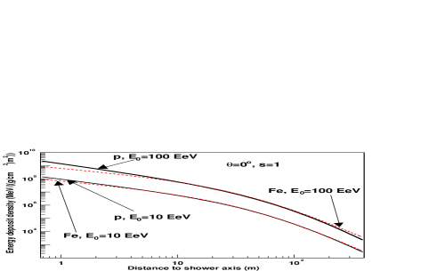
Figure 9: Comparison of the the average lateral distributions of energy deposit density calculated for an average iron and proton showers with different energy.

Average lateral distributions of energy deposit in showers with different primary particle and energy are presented in Figure 9. The lines represent three-parameter fits of NKG-type functions to data points; the parameters are shown in Table 4. The $r_{m}$ and $s$ are only effective fitting parameters, not ”real” Molière radius and age parameter. The NKG function describes the CORSIKA distribution of energy deposit very well close to shower axis, but with non-conventional $r_{m}$ and $s$. It seems that such parameterization will be useful to calculate quickly the fluorescence signal using formula (13). Variation of the parameters ($r_{m}$, $s$) with energy is not strong. For instance, in case of proton showers $r_{m}$ varies by about 2% between $10$ and $100$ EeV and the $s$ parameter varies by about 9%. This means that at first approximation the shape of energy deposit density around the shower maximum seems to be almost independent of energy, although the amount of total energy deposit changes. On the other hand, when we compare $s$ and $r_{m}$ for showers with the same energy but different primary, the differences are much larger.

On the basis of Figure 9, one expects differences in the size of shower image for the same energy, but different primary. To study this effect more precisely, we show in Figure 10B the integral of energy deposit $F_{E}(r)$ for iron and proton shape function at 10 EeV. It can be seen that 90% of energy deposit falls within 125 m from the shower axis in case of proton shower, and within 149 m for iron shower. The image spot size is about 4.5^∘ and 5.4^∘ for proton and iron, respectively. A fit of a functional form as given by Eq. 17 to the fraction of energy deposit in iron showers leads to $a_{Fe}=55.79\pm 1.83$ m and $b_{Fe}=1.805\pm 0.038$ and in proton showers $a_{p}=54.24\pm 1.53$ m and $b_{p}=1.928\pm 0.033$. Thus, the size of shower image for iron showers $\alpha_{Fe}$ and proton one $\alpha_{p}$ can be calculated using formula (18) with appropriate values of parameters; an example is shown in Figure 10C. The size of iron shower image is always larger by about 13% than proton one for all distances. In Figure 10D the relative difference $q=(\alpha_{Fe}-\alpha_{p})/\alpha_{Fe}$ between iron and proton shower image size versus fraction of light is presented. It can be seen that differences in the image spot size between iron and proton increase when we take into account a larger fraction of the energy deposit. We note that the difference $q$ was calculated assuming the same distance to the shower, but not the same altitude of the proton and iron shower maximum. It should therefore be checked if the observed difference between iron and proton image is only an atmospheric effect given by the different local value of $r_{M}$ in air. This atmospheric effect can be estimated using the Molière radius for proton and iron showers at their maxima and can be calculated using the equation $q=1-r_{M,Fe}/r_{M,p}$. Since the Molière radius for iron $r_{M,Fe}=110$ m and for proton $r_{M,p}=104$ m, the relative difference in the shower image due to the atmospheric effect is $q\simeq-6\%$. Thus, half of the difference between the primaries visible in $q$ presented in Figure 10D is caused by this atmospheric effect.

In Figure 11 the influence of fluctuations in proton and iron shower shape function of energy deposit are presented. Fluctuations in proton shower profile lead to changes in the size of the shower image of about $1^{\circ}$. However, the image of a proton shower is always smaller than iron shower image.

3.4 Detailed simulations of the shower image

This section summarizes results presented until now with one modification: we show the shower image including all light components.

Figure 12 shows the size of the shower image $\alpha$ containing $90\%$ or $67\%$ of light as a function of distance $R$ from the FD to the shower, for showers with different core distance $R_{p}$. A comparison of the shower image derived using the two-dimensional CORSIKA histograms and that given by the NKG function is made for two different shower energies. It is evident that the image size in the shower maximum is independent of energy in the NKG approximation and that the NKG approximation leads to larger sizes of shower image than those derived from CORSIKA. Moreover, for a shower with higher energy the image size from CORSIKA is slightly smaller than the size at lower energy. These differences can be understood when we take into account the variation of the shape function in these cases, which were discussed earlier and shown in Figures 3A, 6A and 7A. For example, Figure 7A shows that the values of the shape function at $100$ EeV are larger than those at $10$ EeV at distances to the shower axis smaller than 10 m. Since we calculate the widths of these functions at distances corresponding to $90\%$ or $67\%$ of the total signal, we expect that the width at the higher energy will be smaller. A similar effect is observed when one compares the shape functions in the NKG and CORSIKA approximations, (see Figure 6A). In this case one expects that the width of the shape function in the NKG approximation will be larger than that derived from CORSIKA. In case of the NKG approximation, the changes of the shape functions with energy are negligible, as seen in Figure 3A; the observed small differences are only due to different distances to the shower.

4 Conclusion

Shower image simulations more accurate than available until now are presented, which incorporate a more realistic distribution of fluorescence light emitted by the shower. The image simulations are based on distributions of energy deposited by the shower in air as derived from CORSIKA. A comparison of the size of the shower image obtained using CORSIKA and that given by the NKG function was made for different energies and primary particles. To a first approximation, the results of these two completely independent methods (analytical versus Monte Carlo) show quite reasonable agreement.

The image spot size derived from CORSIKA is smaller by about 15% compared to the NKG approximation. This difference is mainly due to the differences in lateral particle distributions in the NKG and CORSIKA approximation.

The energy deposit distribution from CORSIKA leads to a dependence of the size of shower image on the primary particle, so that studies of the shower image may be helpful for the primary particle identification.

Acknowledgements. We would like to thank R. Engel and F. Nerling for fruitful discussions and careful reading of the manuscript. This work was partially supported by the Polish Committee for Scientific Research under grants No. PBZ KBN 054/P03/2001 and 2P03B 11024 and by the International Bureau of the BMBF (Germany) under grant No. POL 99/013.

Table 1: Average values of depth of first interaction $X_{0}$, depth of shower maximum $X_{max}$ and altitude of shower max $H_{z}$ (above sea level) for vertical showers obtained from CORSIKA.

	$E_{0}$	$X_{0}$	$X_{max}$	$H_{z}$
	(EeV)	(g/cm2)	(g/cm2)	(km)
p	$10$	44.4	757	2.572
	$100$	42.1	805	2.034
Fe	$10$	10.6	696	3.241
	$100$	8.7	746	2.695

Table 2: Size of shower image $\alpha$ and distance $r$ around the shower axis containing $90\%$ and $67\%$ of fluorescence light in the NKG approximation for vertical proton showers of different $E_{0}$ and zenith angle $\theta$ landing at a distance of 3 km from the eye and observed from R=3.16 km. Additionally, the local Molière radius $r_{M}$ is shown at shower maxima.

$E_{0}$	$\theta$	$\alpha_{90\%}$	$r_{90\%}$		$\alpha_{67\%}$	$r_{67\%}$		$r_{M}$
(EeV)	(deg)	(deg)	(m)		(deg)	(m)		(m)
$10$	0	5.69	157		2.10	58		104
$10$	45	7.00	194		2.59	71		128
$100$	0	5.42	150		2.00	55		99
$100$	45	6.68	184		2.47	68		122

Table 3: Size of shower image $\alpha$ and distance $r$ containig $90\%$ and $67\%$ of fluorescence light for vertical proton showers of different zenith angle $\theta$ at energy 10 EeV.

$\theta$	$\alpha_{90\%}$	$r_{90\%}$		$\alpha_{67\%}$	$r_{67\%}$
(deg)	(deg)	(m)		(deg)	(m)
0	4.52	125		1.53	42
45	6.15	170		2.26	65

Table 4: Fitting parameters of NKG-type functions ($r_{m}$, $s$ and $N_{max}$ at shower maximum) to shape functions obtained using CORSIKA lateral distribution of energy deposit. $r_{m}(s=1)$ is the value obtained using fixed values of $s$ parameter at shower maximum.

	$E_{0}$	$r_{m}$	$s$	$N_{max}$	$\chi^{2}/ndf$	$r_{m}$(s=1)	$\chi^{2}/ndf$
	(EeV)	(m)		($10^{10}$ particles)		(m)
p	$10$	$98.1\pm 0.2$	$0.844\pm 0.001$	$1.572\pm 0.001$	3.95	58	4.1
	$100$	$96.7\pm 0.2$	$0.765\pm 0.001$	$16.492\pm 0.004$	2.00	46	8.3
Fe	$10$	$46.5\pm 0.9$	$1.181\pm 0.009$	$1.532\pm 0.001$	1.26	68	1.6
	$100$	$46.6\pm 0.8$	$1.201\pm 0.008$	$15.349\pm 0.008$	1.22	65	1.7

Figure 3: (A) Shape of particle density distribution $f_{{\rm NKG}}(r)$ versus distance to shower axis in the NKG approximation. Showers with different energies $E_{0}$ and zenith angles $\theta$ are shown; (B) Integral $F_{{\rm NKG}}(r)$ of the shape function $f_{{\rm NKG}}(r)$ from Figure 3A. Horizontal dashed lines correspond to 90% and 67%. The vertical dashed line indicates a $1.5^{\circ}$ pixel detector field of view. Upper scale is the shower image size corresponding to distance to shower R=3.16 km. (C) Size of shower image containing 90% of fluorescence light versus the detector-to-shower distance (R).

Figure 4: Relative difference between size of shower image calculated using total light and only fluorescence versus the detector-to-shower (R) distance for a vertical shower with energy 10 EeV.

Figure 6: (A) Shape of particles density $f_{E}(r)$ in the CORSIKA and NKG approximations. (B) Integral $F_{E}(r)$ of shape functions $f_{E}(r)$ from Figure 6A. (C) Size of shower image containing 90% of fluorescence light versus the detector-to-shower distance $R$. (D) Relative difference between shower image size obtained in the CORSIKA and NKG approaches, see text for more details. Vertical showers at energy 10 EeV are presented.

Figure 7: (A) Shape of energy deposit density $f_{E}(r)$ for vertical proton showers with energies 100 EeV and 10 EeV derived from CORSIKA. (B) Integral of energy deposits versus distance to shower axis. (C) Size of shower image containing 90% of fluorescence light versus detector-to-shower distance R. (D) Relative difference in the shower image size between proton showers with energies 10 EeV and 100 EeV.

Figure 8: (A) Integral of energy deposits versus distance to shower axis for proton showers with different inclination, derived from CORSIKA. (B) Relative difference in the shower size image between these showers.

Figure 10: (A) Shape of energy deposit density $f_{E}(r)$ for vertical 10 EeV proton and iron showers. (B) Integral of energy deposit versus distance to shower axis for proton shower (solid line) and iron (dashed line). (C) Size of shower image containing 90% of fluorescence light versus detector to shower distance $R$. (D) Relative difference in the shower image between iron and proton shower.

Figure 11: (A) Lateral distribution of energy deposit calculated for 15 single proton showers (solid lines) and average of 5 iron showers (dashed lines) at energy $E_{0}=10$ EeV. (B) Integral of the energy deposits versus distance to shower axis for proton showers (solid lines) and iron ones (dashed line).

Figure 12: (A) Size of the shower image at shower maximum containing 90% and 67% of light versus the detector to shower distance $R$, using the CORSIKA and NKG distributions of energy deposit. The dashed line corresponds to shower image obtained with constant value of fluorescence yield $n_{\gamma,0}=4.02$ photons/m. (B) Size of the shower image containing 90% and 67% of light versus $R$ using the CORSIKA distributions of energy deposit for iron (showers at different energies).

References

- [1] T. K. Gaisser and A. M. Hillas, Proc. 15th ICRC, Plovdiv, 8 353 (1977).
- [2] R. M. Baltrusaitis et al., Nucl. Instr. Meth. A240 410 (1985).
- [3] P. Sommers, Astropart. Phys. 3 349 (1995)
- [4] D. Heck et al., Report FZKA 6019, Forschungszentrum Karlsruhe, (1998).
- [5] D. Góra et al., Astropart. Phys. 16 129 (2001).
- [6] M. Giller et al., Astropart. Phys. 18 513 (2003)
- [7] M. Risse and D. Heck, Astropart. Phys. 20 661 2004; preprint astro-ph/0308158 (2003)
- [8] P. Homola et al., Pierre Auger Project Note GAP-2001-036 (2001).
- [9] B. Dawson, private communication (1998).
- [10] V. Souza, H. M. J. Barbosa, and C. Dobrigkeit, preprint astro-ph/0311201 (2003)
- [11] F. Kakimoto et al., Nucl. Instr. Meth. A 372 527 (1996).
- [12] A. N. Bunner, PhD Thesis, Cornell University, Ithaca, NY, USA (1967).
- [13] M. Nagano et al., Astropart. Phys. 20 293 (2003); preprint astro-ph/0303193.
- [14] R. M. Baltrusaitis et al., Proc. ICRC, La Jolla, 7 159 (1985).
- [15] K. Kamata et al., Suppl. Progr. Theor. Phys., 6 93 (1958)
- [16] K. Greisen, Prog. Cosmic Ray Phys. 1 (1956); J.A.J. Matthews, Pierre Auger Project Note GAP-1998-002 (1998).
- [17] M. Abramowitz and I. A. Stegun, (Eds.) Handbook of Mathematical Functions, New York, Dover Publications, Inc. (1965).
- [18] D. Heck and J. Knapp, Report FZKA 6097, Forschungszentrum Karlsruhe, (1998).
- [19] W. R. Nelson, H. Hirayama and D. W. O. Rogers , Report SLAC 265 (1985).
- [20] N. N. Kalmykow, S. S. Ostapchenko, and A. I. Pavlov, Nucl. Phys. B (Proc. Suppl.) 52B 17 (1997).
- [21] M. Hillas, Nucl. Phys. B (Proc. Suppl.) 52B 29 (1997).
- [22] M. Kobal et al., Proc. ICRC, Salt Lake City, 1 490 (1999). M. Kobal, Astropart. Phys. 15 259 (2001).
- [23] M. Risse et al., Proc. 27th ICRC, Hamburg, 2 522 (2001).