Markov Chain Monte Carlo joint analysis of Chandra X-ray imaging spectroscopy and Sunyaev-Zeldovich Effect data

Abstract

X-ray and Sunyaev-Zeldovich Effect data can be combined to determine the distance to galaxy clusters. High-resolution X-ray data are now available from the Chandra Observatory, which provides both spatial and spectral information, and Sunyaev-Zeldovich Effect data were obtained from the BIMA and OVRO arrays. We introduce a Markov chain Monte Carlo procedure for the joint analysis of X-ray and Sunyaev-Zeldovich Effect data. The advantages of this method are the high computational efficiency and the ability to measure simultaneously the probability distribution of all parameters of interest, such as the spatial and spectral properties of the cluster gas and also for derivative quantities such as the distance to the cluster. We demonstrate this technique by applying it to the Chandra X-ray data and the OVRO radio data for the galaxy cluster Abell 611. Comparisons with traditional likelihood-ratio methods reveal the robustness of the method. This method will be used in follow-up papers to determine the distances to a large sample of galaxy clusters.

1 Introduction

Analysis of Sunyaev-Zeldovich Effect (SZE) and X-ray data provides a unique method of directly determining distances of galaxy clusters. Clusters of galaxies contain hot plasma ($k_{B}T_{e}\sim$ 2-20 keV) that scatters the cosmic microwave background radiation (CMB). On average, this inverse Compton scattering boosts the energy of the CMB photons, causing a small distortion in the CMB spectrum (Sunyaev and Zeldovich 1970,1972). For recent reviews of the SZE and its application for cosmology see Birkinshaw (1999) and Carlstrom et al. (2002).

The SZE is proportional to the integrated pressure along the line of sight, $\Delta T\propto\int n_{e}T_{e}dl$, where $n_{e}$ and $T_{e}$ are the electron density and electron temperature of the cluster plasma. The thermal X-ray emission from the same plasma has a different dependence on the density, $S_{x}\propto\int n_{e}^{2}\Lambda_{ee}dl$, where $\Lambda_{ee}$ is the X-ray cooling function. Making assumptions on the distribution of the plasma (e.g., a $\beta$ profile) and taking advantage of the different dependence on $n_{e}$, SZE and X-ray observations can be combined to determine the distance to galaxy clusters. These cluster distances can be combined with redshift measurements to determine the value of the Hubble constant (Myers et al. 1997, Grainge et al. 2002, Reese et al. 2002).

In this paper we introduce a Markov chain Monte Carlo (MCMC) procedure for the joint analysis of SZE and X-ray data. The method is tested on the galaxy cluster Abell 611 which has SZE data obtained with the Caltech millimeter interferometric array at the Owens Valley Radio Observatory (OVRO) outfitted with centimeter-wave receivers (Carlstrom, Joy and Grego 1996) and X-ray data from the Chandra X-ray Observatory. In a subsequent paper we will report the application of this technique to a sample of $\sim$40 clusters.

2 Data

2.1 Chandra X-ray data

The Advanced CCD Imaging Spectrometer (ACIS) on board the Chandra X-ray Observatory provides high angular resolution (half-power radius $\sim 0.5$ arcsec) and good spectral resolution (50-300 eV FWHM) in the $\sim 0.3-10$ keV energy range. We use the following steps to reduce the raw (Level 1) Chandra data:
(a) We use the ‘acis_process_events’ tool from the Chandra Interactive Analysis of Observations (CIAO) package to correct the Level 1 data for charge transfer inefficiency.
(b) We generate a Level 2 event file applying standard filtering techniques: we select grade=0,2,3,4,6, status=0 events and filter the event file for periods of poor aspect solution using the good time interval (GTI) data.
(c) Periods of high background count rates are occasionally present, typically due to Solar flares (Markevitch 2001). We discard these periods by constructing a light-curve of a detector region devoid of astronomical sources, using a bin length of 500 seconds. Time intervals that are in excess of the median count rate by more than 4$\sigma$ are considered to be affected by high background levels, and are discarded from the dataset. This method is similar to that employed by Markevitch (2001) for the study of blank-sky fields.
(d) We extract the cluster spectrum out to a radius that encompasses 95% of the cluster counts. The 95% radius is determined by extracting counts in annuli around the cluster center, and forming the cumulative distribution. All detectable point sources in the X-ray image are excluded.

Background in the ACIS instrument includes detector and astronomical components (see Markevitch et al. 2003). The background is particularly time-variable in the lowest energy channels (E$\leq$ 0.7 keV; Snowden et al. 1998). At the highest energies, the cluster emission decreases and the signal becomes background-dominated. For these reasons, we limit our analysis to the 0.7-7 keV range; this band includes the Fe complex lines at $\sim$ 6.7 keV (in the rest frame) which are necessary for an accurate determination of the plasma metallicity.

2.1.1 Chandra observations of Abell 611

The X-ray data were obtained with the ACIS-S detector on the Chandra observatory on Nov. 3, 2001 (OBS ID 3194), with a total on-source time of 36,599 s. The detector operating temperature was -120 C. Periods of high background and poor aspect solution were filtered out, resulting in a total effective exposure time of 36,114 s.

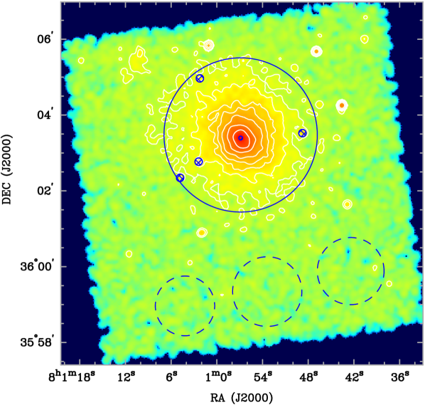
Figure 1: Chandra 0.7-7 keV image of Abell 611. Image is not exposure corrected, contours are 0.5, 1, 2, 3, 5, 9 and 15 counts/pixel, pixel size is 1.97 arcsec. The image was smoothed with a Gaussian kernel of $\sigma$=4 arcsec. The solid circle encompasses 95% of the cluster counts and cross-hatched areas were excluded due to point source contamination. Dashed circles are the regions used for background determination.

In Fig. 1 we show the ACIS-S3 image of the cluster, smoothed with a Gaussian kernel of $\sigma$=4 arcsec. The blue solid circle is the region used for the spectral extraction, cross-hatched areas are the excluded regions and the blue dashed circles are the regions used for background determination. Among the excluded regions is the cD galaxy 2MASX J08005684+3603234 (Crawford et al. 1999). The X-ray background level was 8.6$\times 10^{-6}$ counts cm^-2 arcmin^-2 s^-1. We assume a Galactic HI column density of $N_{H}=5.0\times 10^{20}$ cm^-2 (Dickey and Lockman 1990) in the spectral analysis of the X-ray data.

2.1.2 Background subtraction

We investigate the ACIS background through the analysis of two collections of blank-sky exposures (acis57D2000-01-29bkgrndN0003.fits and acisiD2000-01-29bkgrndN0002.fits) provided with the CIAO software for the purpose of background estimation. The two datasets have exposure times of respectively 54 ks and 450 ks. Several other blank-sky observations are available which cover the entire life span of the Chandra mission.

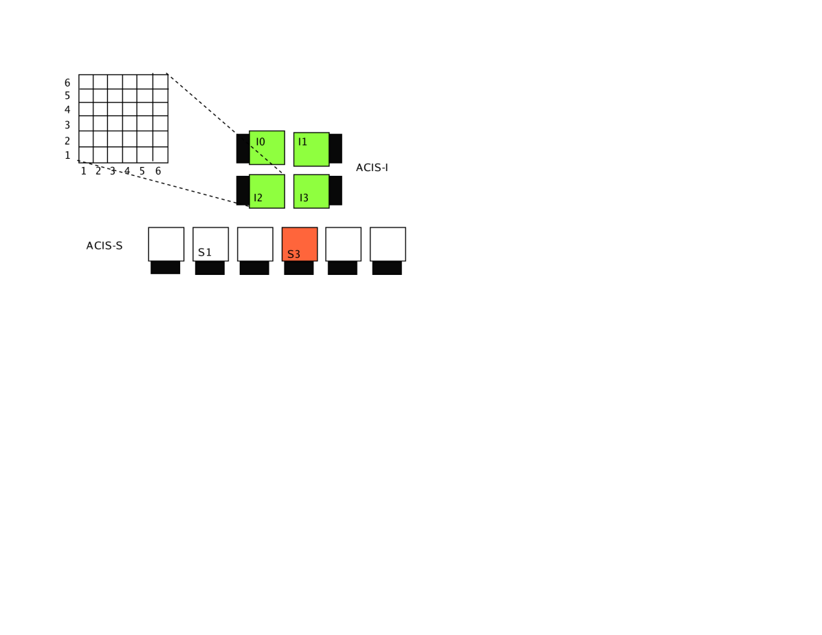
Figure 2: Layout of the ACIS detector, not to scale. Each CCD is divided into 36 zones to study the spatial behavior of the response.

The ACIS instrument is comprised of 10 CCDs on the focal plane of the Chandra telescope. A layout of the ACIS instrument is shown in Fig. 2 (see the Chandra Proposer’s Observatory Guide for further details). For each of the S3, I0, I1, I2, and I3 CCDs, we select only events in the 0.7-7 keV energy range from the two blank-sky observations. The linear size of each CCD is approximately 8 arcmin. We divide each CCD into a 6x6 grid, as indicated in Fig. 2, to investigate the spatial variation of each CCD’s response.

The S3 CCD has small spatial fluctuations in the detected counts, with a standard deviation for the 36 regions that is 7.1 % of the mean. We conclude that the ACIS-S3 CCD has a flat response, and that the background can be simply estimated from a portion of the CCD which is devoid of celestial sources (e.g., the galaxy cluster or other point sources).

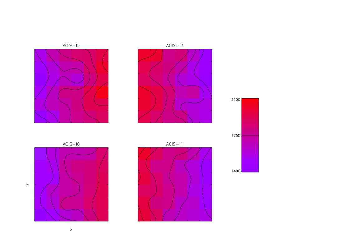
Figure 3: Spatial behavior of the ACIS-I response in 0.7-7 keV band. Counts from the 450 ks blank-field exposure (see text for details) were accumulated in $\sim 1.4\times 1.4$ square arcmin pixels.

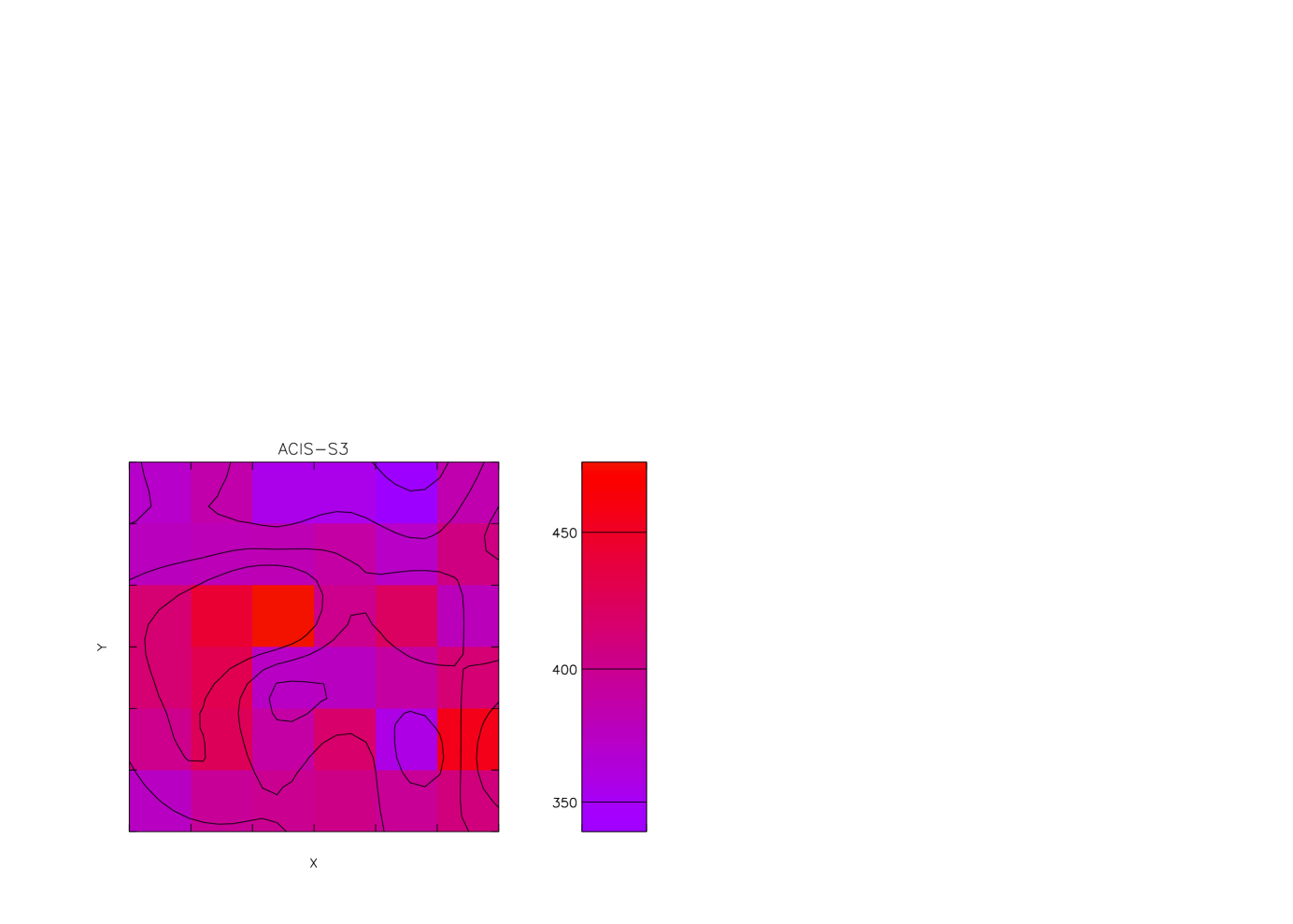
Figure 4: Spatial behavior of the ACIS-S3 response in 0.7-7 keV band. Counts from the 54 ks blank-field exposure (see text for details) were accumulated in $\sim 1.4\times 1.4$ square arcmin pixels.

The situation is different for the ACIS-I CCDs. In all four ACIS-I CCDs the response increases with distance from the read-out nodes, depicted as black rectangles in Fig. 2. This gradient in the response is at the level of 25 %, and it results in a standard deviation of about 10 % of the mean of the counts for all CCDs, as shown in Fig. 3. No such gradient is present in the S3 data, as shown in Fig. 4. Similar results were found by Markevitch (2001) using other blank-field Chandra exposures. Since the gradient and the absolute response are similar in all four ACIS-I CCDs, the background can be estimated by using any (or all) of the CCDs that are not contaminated by the cluster emission. The aimpoint of the ACIS-I observations is on CCD I3, and CCDs I0, I1 and I2 are typically free of cluster emission.

Our background estimation technique therefore consists of selecting a region devoid of astronomical sources from the same cluster observation, according to the following scheme:
(a) If the observation is performed with the ACIS-S configuration, the background is chosen from peripheral regions of the same ACIS-S3 CCD where the cluster is detected.
(b) If the observation uses the ACIS-I configuration, the background is chosen from the 3 CCDs (I0,I1 and I2) that are near the I3 CCD where the cluster aimpoint is located. The background region is at the same distance from the read-out nodes as the cluster. This is the case of several observations to be presented in follow-up papers.

2.2 Interferometric SZE data

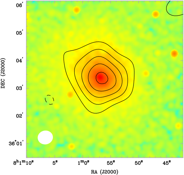
Figure 5: SZE contours overlaid on the Chandra 0.7-7 keV image of Abell 611. The rms noise is 40 $\mu$Jy/beam and the contours are at -5, -4, -3, -2, -1 and 1$\times 112$ $\mu$Jy/beam; negative (positive) contours are shown as solid (dashed) lines. The synthesized beam is 62x56 arcsec.

The SZE measurements discussed in this paper were obtained by outfitting the 6-element OVRO millimeter array with centimeter wavelength receivers (Carlstrom, Joy and Grego 1996). The details of the observations and data reduction are covered extensively in Reese et al. (2002) and only reviewed briefly here. The data were taken with two 1 GHz wide bands centered at 29 GHz and 30GHz with receiver temperatures $T_{rx}\sim$ 11-20 K. The typical system temperatures scaled to above the atmosphere were $T_{sys}\sim$ 45 K. Multiple configurations of the telescopes were used which typically placed most of the telescopes in a compact configuration to maximize the sensitivity on the angular scale of distant galaxy clusters ($\sim$ 1 arcmin), but with a subset of the telescopes forming longer baselines to provide simultaneous detection (and subsequent removal) of radio background point sources. Abell 611 was observed with the OVRO array for a total of 57 hours. The SZE data were reduced using the MMA software package (Scoville et al. 1993). No point sources were found with a 3$\sigma$ upper limit of $135\mu$Jy (not corrected for attenuation by the $4.2^{\prime}$ FHWM primary beam). In Fig. 5 we show a contour plot of the SZE data overlaid on the Chandra X-ray image.

3 Obtaining cluster distances

The high computational efficiency of the MCMC analysis and the improvements in the X-ray and SZE data will allow more complex models for the instracluster gas. To demonstrate the MCMC analysis, however, we follow the procedure detailed by Reese et al. (2002). We assume that the spatial distribution of the cluster plasma is described by a spherical isothermal $\beta$-model (Cavaliere and Fusco-Femiano 1976, 1978) given by:

$$n_{e}(r)=n_{e0}\left(1+\frac{r^{2}}{r_{c}^{2}}\right)^{-\frac{3\beta}{2}}$$ (1)

where $n_{e}$ is the electron number density, $r$ is the radius from the cluster’s center, $r_{c}$ is the core radius and $\beta$ is a power-law index. With this model, the thermodynamic SZE temperature decrement/increment $\Delta T$ is

$$\Delta T=f_{(x,T_{e})}T_{CMB}D_{A}\int d\zeta\sigma_{T}n_{e}\frac{k_{B}T_{e}}{m_{e}c^{2}}=\Delta T_{0}\left(1+\frac{\theta^{2}}{\theta_{c}^{2}}\right)^{\frac{1-3\beta}{2}}$$ (2)

where $f_{(x,T_{e})}$ is the frequency dependence of the SZE with $x=\frac{h\nu}{k_{B}T_{CMB}}$ (e.g., Reese et al. 2002 and references therein), $D_{A}$ is the cluster angular diameter distance, $T_{CMB}$=2.728 K (Fixsen et al. 1996), $\theta$ is the angular radius in the plane of the sky, $\theta_{c}$ the corresponding angular core radius, $\sigma_{T}$ is the Thomson cross section, $k_{B}$ is Boltzmann’s constant, $c$ is the speed of light in vacuo, $m_{e}$ is the electron’s mass and $T_{e}$ the electron’s temperature. The integration is performed along the line of sight, $l$, and we define $\zeta=l/D_{A}$.

The X-ray surface brightness is given by

$$S_{X}=\frac{1}{4\pi(1+z)^{4}}D_{A}\int d\zeta n_{e}^{2}\Lambda_{ee}=S_{X0}\left(1+\frac{\theta^{2}}{\theta_{c}^{2}}\right)^{\frac{1-6\beta}{2}}$$ (3)

where $S_{X}$ is the surface brightness, $z$ is the cluster’s redshift and $\Lambda_{ee}=\Lambda_{ee}(T_{e},A)$ is the X-ray cooling function of the gas.

Eq. 2 and 3 can be combined to determine $D_{A}$:

$$D_{A}=\frac{\Delta T_{0}^{2}}{S_{X0}}\left(\frac{m_{e}c^{2}}{k_{B}T_{e0}}\right)^{2}\frac{\Lambda_{ee}}{4\pi f^{2}_{(x,T_{e})}T^{2}_{CMB}\sigma^{2}_{T}(1+z)^{4}}\frac{1}{\theta_{c}}\left[\frac{\Gamma(3\beta/2)}{\Gamma(3\beta/2-1/2)}\right]^{2}\frac{\Gamma(3\beta-1/2)}{\Gamma(3\beta)}$$ (4)

where $\Gamma()$ is the gamma function which comes from the integration of the $\beta$-model along the central line of sight. Similarly, one can eliminate $D_{A}$ to obtain $n_{e0}$ (e.g., Reese et al. 2002; Birkinshaw 1999).

4 Joint SZE and X-ray data modelling

The SZE and the X-ray emission both depend on the properties of the hot cluster plasma. We use a joint model for the interferometric SZE radio data and the Chandra X-ray data which describes all the relevant spatial and spectral characteristics necessary for the distance measurement. The model consists of:
(a) A $\beta$-model of the plasma distribution (see Eq. 2 and 3). The model includes the variable parameters $S_{X0}$, $\beta$, $r_{c}$, $\Delta T_{0}$, and the fixed coordinates of the cluster center.
(b) A photoabsorbed optically-thin spectral model (Raymond-Smith and WABS models in XSPEC) to determine $T_{e}$ and metal abundance $A$ of the gas. Solar metal abundances are from Feldman (1992). The cluster plasma is assumed to be isothermal.
(c) Additional parameters: the X-ray background level, held fixed at its measured value (see sec. 2.1.1) and, if present, the position and flux of radio point sources. No radio point sources are found in the SZE data for A611.

In summary, the model is described by a set of parameters $\theta$ $\equiv$($\beta$, $r_{c}$, $\Delta T_{0}$, $S_{X0}$, $T_{e}$, $A$). For each parameter set $\theta$, we calculate the joint likelihood $\mathcal{L}$ (e.g., Bevington 1969) of the model with the available data. Since the datasets (SZE and X-ray) are independent, the joint likelihood is the product of the individual likelihoods.

The interferometric SZE data provide constraints in the Fourier u-v plane, and the likelihood of the SZE dataset is therefore directly calculated in u-v coordinates (see Reese et al. 2000). The likelihood of the X-ray images is calculated pixel by pixel. For the spectral X-ray data, an analytical model of the emissivity (available through the XSPEC software) is convolved with the Chandra response, and the likelihood is calculated in each spectral channel.

We employ the computationally efficient Markov chain Monte Carlo method in order to handle the large numbers of parameters involved in the joint SZE/X-ray spatial and spectral analysis.

4.1 The Markov chain method

The Markov chain Monte Carlo method can be used to obtain the probability distribution function of model parameters based on observational data (Gamermann 1997, Gilks, Richardson and Spiegelhalter 1996, Christensen and Meyer 2001, Lewis and Bridle 2002, MacKay 2003, Marshall, Hobson and Slosar 2003, Hobson and McLachlan 2003, Verde et al. 2003, Christensen et al. 2001). To create the Markov chain, we choose candidate parameter values ($\theta^{\prime}$) from the allowed parameter space (the parameter support, Table 1). The support values in Table 1 were determined from test runs of the Markov chain with very broad parameter limits to ensure that all statistically acceptable regions of parameter space were included.

Given these candidate parameters, we compute the likelihood of the model and the candidates are either accepted or rejected based on the Metropolis-Hastings acceptance algorithm (Metropolis et al. 1953; Hastings 1970; Gilks, Richardson and Spiegelhalter 1996). When a sufficiently large number of parameters has been accepted into the Markov chain, the frequency of their occurrence in the chain approaches the true probability distribution function (Gamermann 1997, Gilks, Richardson and Spiegelhalter 1996, MacKay 2003).

4.2 Proposal distribution and starting point

In constructing a MCMC one has the freedom to choose any desired method for drawing candidates (Roberts 1996; MacKay 2003). We draw candidates $\theta^{\prime}$ that are in the neighborhood of the previously accepted parameters, instead of drawing them from the full parameter space. Our ‘proposal’ distribution is a simple top-hat function. A small width for the proposal distribution typically results in a high acceptance rate, as candidates have a likelihood that is similar to that of the previously accepted parameters. On the other hand, a large number of steps is required for the Markov chain to sample the entire parameter space. We tested proposal distribution widths from 10% to 50% of the parameter support (see Table 1), calculated the number of iterations required for convergence (see the following section) and present the results in Table 2. The optimum proposal distribution width is approximately 25%, and we use this value for all subsequent analysis.

The starting point of a Markov chain can be chosen arbitrarily (e.g., Gilks, Richardson and Spiegelhalter 1996). We start the Markov chain at the midpoint of each parameter’s support (see Table 1), and run the Markov chain for 100,000 iterations. The acceptance rate for a 25% proposal distribution width is 11.4%.

4.3 Convergence of the Markov chain

A Markov chain requires a large number of steps before it reaches convergence. We test the convergence using three independent tests: the Raftery-Lewis diagnostic (Raftery and Lewis 1992), the Gelman-Rubin diagnostic (Gelman and Rubin 1992) and the Geweke test (Geweke 1992; Gamermann 1997; Geyer 1992).

The Raftery-Lewis method determines whether convergence to the stationary distribution has been achieved, and also estimates the number of iterations that are required in order to determine confidence intervals to a specified accuracy. We used the CODA routines (Best, Cowles, and Vines, S.K. 1995, Plummer et al. 2004) to compute the Raftery-Lewis statistics, and present the results in Table 3. For all of the parameters, the number of iterations required is less than our chain length of 100,000.

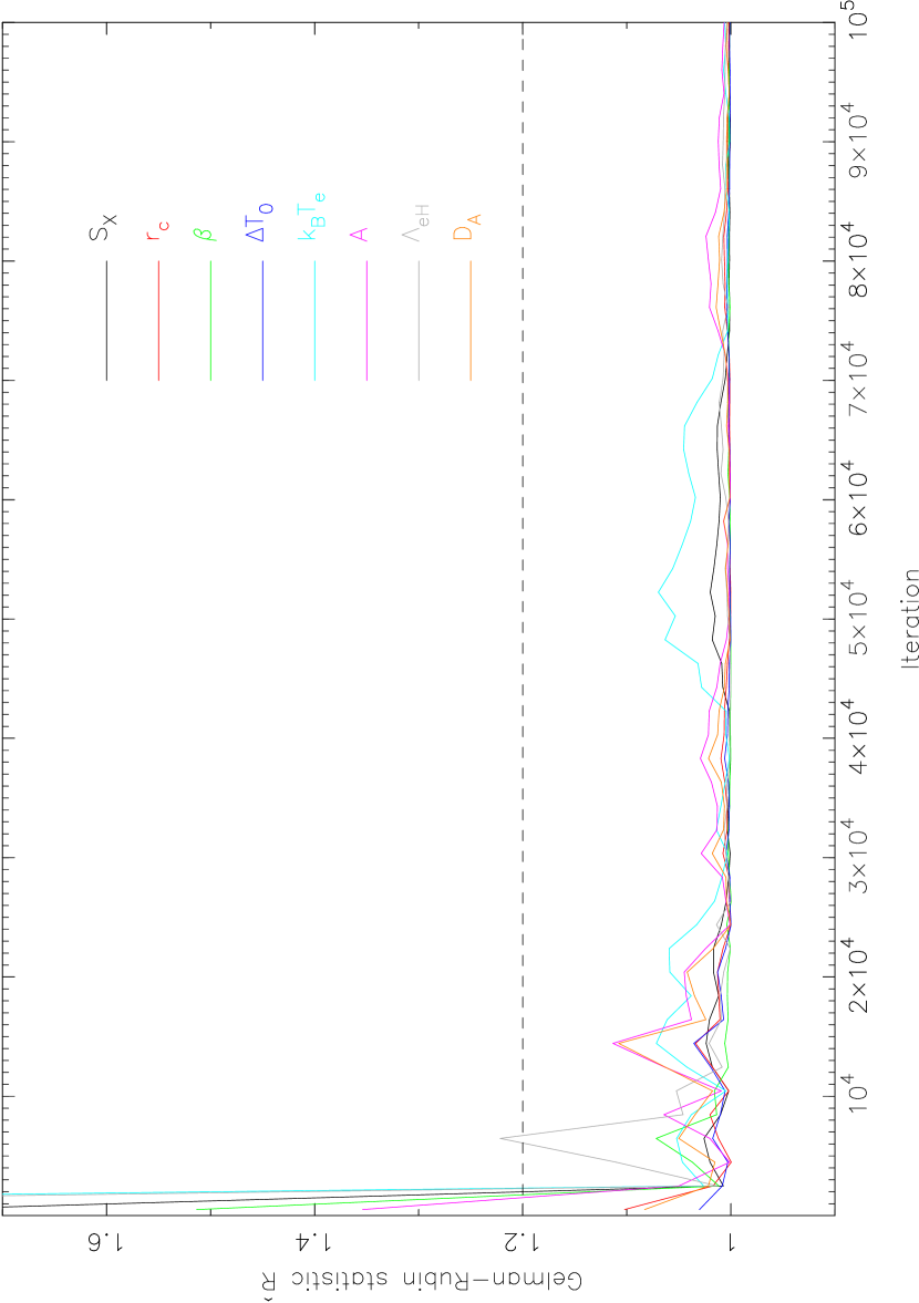
Figure 6: Gelman-Rubin statistic $\hat{R}$ obtained from 3 simultaneous Markov chains with different initial conditions.

The Gelman-Rubin test is based on several parallel Markov chains, each started from different initial values. The method calculates a factor, $\hat{R}$, based on the variance within and between each chain. Convergence is indicated by $\hat{R}\lesssim$ 1.2 (Gelman 1996). Fig. 6 shows the Gelman-Rubin statistic computed from three parallel chains; the test indicates that convergence is achieved early in our 100,000 element chain.

Finally, we compute the Geweke $z_{G}$ statistic. We discard the initial $n_{i}$=5,000 steps of the chain (the burn-in period), and divide the remaining $n$=95,000 steps into the initial 10% ($n_{b}=9,500$) and the final 50% ($n_{a}=47,500$) segments, according to Geweke (1992). The intermediate 40% portion in not used for testing the convergence. Since the values in the Markov chain are correlated by construction, the initial and final segments are averaged over 100 steps, to ensure that the rebinned values are uncorrelated (Roberts 1996). The $z_{G}$ function, also known as the Geweke z-score, is the standardized difference between the initial and the final portions of the chain, and it is distributed as a standard Gaussian N(0,1) if the chain has reached convergence. Convergence is therefore indicated if $z_{G}$ values are less than $\sim 3\sigma$ for all parameters (Geweke 1992; Gamerman 1997). The $z_{G}$ values for our Markov chain are shown in Table 3, and are all within $\pm 2\sigma$, consistent with convergence to the stationary distribution.

4.4 Results of the Markov chain Monte Carlo for Abell 611

In Fig. 7 we show the probability distribution functions for all parameters. The 68% and 90% confidence intervals (calculated by marginalizing over all other parameters) are given in Table 4.

Thinning the Markov chain is often employed to weed out values which are highly correlated with neighboring elements in the chain. To examine the effect this would have on the derived confidence intervals, we selected every tenth element in the chain and recalculated the statistics. The results (right side of Table 4) indicate that there is no significant change in the derived confidence intervals. Finally, we calculated the correlation coefficients between parameters, and the results are shown in Table 5. As expected, parameters $r_{c}$ and $\beta$ are strongly correlated (see Reese et al. 2002, Grego et al. 2001).

4.5 Comparison with other analysis methods

We employ the XSPEC spectral code to compare the confidence intervals on the spectral parameters $T_{e}$ and $A$. Table 6 shows the comparison between the MCMC-derived best-fit values and confidence intervals with those provided by XSPEC. The results are in excellent agreement, confirming our MCMC results. In addition, we use the CIAO Sherpa software to determine the $\beta$-model parameters, and results are also shown in Table 6. The agreement with the results of Table 4 provides additional confidence in the reliability of our analysis.

Abell 611 data were also analyzed by Reese et al. (2002). Using the same SZE data, but lower resolution ROSAT and ASCA X-ray data, they found a SZE decrement of $\Delta T_{0}=-853\pm^{120}_{140}\;\mu$K. Our results of $\Delta T_{0}=-801\pm{84}\;\mu$K are again in very good agreement with theirs.

5 Conclusions

We present a Markov chain Monte Carlo technique to derive cluster distances from SZE and X-ray data. The method was succesfully tested on the OVRO and Chandra data of Abell 611, a galaxy cluster at z=0.288. We measure an angular diameter distance of $D_{A}=1.00\pm^{0.24}_{0.21}$ Gpc (68% confidence level). In a previous work based on the same SZE data, but using lower-resolution X-ray data, Reese et al. (2002) derived a distance of $D_{A}=0.99\pm^{0.32}_{0.29}$ Mpc.

The Chandra X-ray data provides simultaneous spatial and spectral information, featuring the finest angular resolution to date ($\sim 0.5$ arcsec half-power radius). The MCMC method has two major advantages: it is computationally more efficient than the traditional likelihood ratio-based methods and it provides simultaneously the probability distribution function of all model parameters.

This technique will be used in future papers to determine the distances of a large sample of galaxy clusters for which there are available high-resolution Chandra X-ray data and BIMA/OVRO SZE data.

This work is supported by NASA LTSA grant NAG 5-7986. E.D.R. acknowledges support from NASA Chandra Postdoctoral Fellowship PF 1-20020. Partial support was also provided by NSF grants AST-0096913 and PHY-0114422. S.J.L. acknowledges support from NASA GSRP Fellowship NGT5-50173. We thank the referee for helpful comments and suggestions.

Table 1: Parameters in the Markov chain Monte Carlo

Parameter	Starting value	Lower limit	Upper limit	Units
$S_{X0}$	1.02	0.89	1.16	$10^{-3}$ counts s-1 cm-2 arcmin-2
$r_{c}$	20	17	23	arcsec
$\beta$	0.59	0.56	0.62	–
$\Delta T_{0}$	-0.80	-1.10	-0.50	mK
$k_{B}T_{e}$	6.25	5	7.5	keV
$A$	0.35	0.1	0.6	solar

Table 2: Number of iterations required for convergence as a function of proposal distribution width

Parameter	Proposal distribution width
	10%	20%	25%	30%	50%
$S_{X0}$	113680	60885	29190	50256	91122
$r_{c}$	165540	68498	86906	47957	101375
$\beta$	118503	64832	73780	61800	97292
$\Delta T_{0}$	101200	73270	40185	50892	97379
$k_{B}T_{e}$	68180	74148	32916	92579	99748
$A$	129903	49358	89360	38143	89423
$\Lambda_{ee}$	99160	59080	65918	52810	100557
$D_{A}$	88480	67312	62899	53478	106959

Note. — The number of iterations required for convergence are obtained from the Raftery-Lewis test, for a 68% confidence interval (see Table 3).

Table 3: Markov chain Convergence Tests

	Raftery-Lewis		Raftery-Lewis		Geweke
	(68% C.I.)		(90% C.I.)
	Burn-in	Iterations required	Burn-in	Iterations required	$z_{G}$
Parameter	Iterations	for convergence	Iterations	for convergence
$S_{X0}$	108	29190	97	36518	0.78
$r_{c}$	304	86906	225	78690	-0.84
$\beta$	280	73780	138	51794	-0.80
$\Delta T_{0}$	147	40185	137	51595	1.45
$k_{B}T_{e}$	122	32916	95	35775	0.34
$A$	320	89360	171	67583	-1.12
$\Lambda_{ee}$	253	65918	160	58176	-1.03
$D_{A}$	248	62899	109	40924	-1.59

Note. — We used the CODA software to calculate the Raftery-Lewis statistics. For the 68% confidence interval (corresponding to the q=0.16 quantile), we required an accuracy of r=2% with a probability of s=90%. For the 90% confidence interval (q=0.05 quantile), we required an accuracy of r=1% with a probability of s=90%.

Table 4: Markov chain Monte Carlo results for Abell 611 data

	FULL CHAIN			THINNED CHAIN
Parameter	Median	68 % interval	90 % interval	Median	68 % interval	90 % interval
$S_{X0}$	1.02	$\pm^{0.03}_{0.03}$	$\pm^{0.05}_{0.05}$	1.02	$\pm^{0.03}_{0.03}$	$\pm^{0.05}_{0.05}$
$r_{c}$	20.00	$\pm^{0.70}_{0.62}$	$\pm^{1.14}_{1.10}$	20.00	$\pm^{0.69}_{0.61}$	$\pm^{1.14}_{1.02}$
$\beta$	0.594	$\pm^{0.008}_{0.007}$	$\pm^{0.013}_{0.012}$	0.594	$\pm^{0.006}_{0.007}$	$\pm^{0.013}_{0.012}$
$\Delta T_{0}$	-0.801	$\pm^{0.084}_{0.083}$	$\pm^{0.133}_{0.139}$	-0.800	$\pm^{0.082}_{0.082}$	$\pm^{0.132}_{0.140}$
$k_{B}T_{e}$	6.25	$\pm^{0.30}_{0.28}$	$\pm^{0.50}_{0.43}$	6.25	$\pm^{0.30}_{0.28}$	$\pm^{0.50}_{0.42}$
$A$	0.34	$\pm^{0.07}_{0.07}$	$\pm^{0.12}_{0.12}$	0.34	$\pm^{0.07}_{0.07}$	$\pm^{0.07}_{0.07}$
$\Lambda_{ee}$	2.26	$\pm^{0.03}_{0.03}$	$\pm^{0.06}_{0.05}$	2.26	$\pm^{0.03}_{0.03}$	$\pm^{0.06}_{0.04}$
$D_{A}$	1.00	$\pm^{0.24}_{0.21}$	$\pm^{0.43}_{0.33}$	1.01	$\pm^{0.24}_{0.21}$	$\pm^{0.42}_{0.33}$

Note. — Units of measure for $\Lambda_{ee}$ are counts cm³ s^-1, and $D_{A}$ is measured in Gpc. For units of measure of all other quantities, see Table 1.

Table 5: Correlation coefficients for parameters in Markov chain Monte Carlo

$\begin{array}[]{r|rrrrrrrr}&S_{X0}&r_{c}&\beta&\Delta T_{0}&A&k_{B}T_{e}&\Lambda_{ee}&D_{A}\\ \hline\cr S_{X0}&1.00&-0.86&-0.64&-0.10&0.02&0.03&0.03&-0.02\\ r_{c}&&1.00&0.93&0.14&-0.01&-0.04&-0.02&-0.01\\ \beta&&&1.00&0.15&-0.00&-0.04&-0.02&-0.03\\ \Delta T_{0}&&&&1.00&-0.01&-0.00&-0.01&-0.90\\ A&&&&&1.00&-0.15&0.93&0.13\\ k_{B}T_{e}&&&&&&1.00&0.22&-0.40\\ \Lambda_{ee}&&&&&&&1.00&-0.02\\ D_{A}&&&&&&&&1.00\\ \end{array}$

Table 6: Comparison of Markov chain Monte Carlo results with XSPEC and CIAO Sherpa results

Parameter	68% interval	68% interval
	(MCMC)	(XSPEC/Sherpa)
$k_{B}T_{e}$	6.23$\pm^{0.29}_{0.29}$	6.20$\pm{0.30}$ (XSPEC)
$A$	0.34$\pm^{0.07}_{0.07}$	0.35$\pm^{0.07}_{0.08}$ (XSPEC)
$S_{X0}$	1.02$\pm^{0.03}_{0.03}$	1.07$\pm^{0.03}_{0.03}$ (Sherpa)
$r_{c}$	20.00$\pm^{0.70}_{0.62}$	19.42$\pm{0.63}$ (Sherpa)
$\beta$	0.594$\pm^{0.008}_{0.007}$	0.589$\pm{0.01}$ (Sherpa)

Note. — The CIAO Sherpa spatial fit is based only on the Chandra X-ray data, not the combination of X-ray and radio data, as in Table 4. We determined, however, that the results of Table 4 are virtually unchanged when the X-ray data alone are used for the determination of the beta model; the high S/N X-ray data drive the fit of the spatial parameters.

Figure 7: Results of the Markov chain for all parameters Top: Probability distribution. We excised the initial 5,000 events, and used 95,000 events to determine the distribution. Bottom: Time series of the Markov chain including all 100,000 events.

References

- (1) Best, N.G., Cowles, M.K. and Vines, S.K. 1995, CODA Manual version 0.30, MRC Biostatistic Unit, Cambridge, UK
- (2) Bevington, P.R. 1969, Data reduction and error analysis for the physical sciences, McGraw-Hill
- (3) Birkinshaw, M. 1999, Phys. Rep., 310, 97
- (4) Carlstrom, J.E., Holder, G.P. and Reese, E.D. 2002, ARA&A40, 643
- (5) Carlstrom, J.E., Joy, M.K. and Grego, L. 1996, ApJ, 456, 75
- (6) Cavaliere, A. and Fusco-Femiano, R. 1976, A&A, 49, 137
- (7) Cavaliere, A. and Fusco-Femiano, R. 1978, A&A, 70, 677
- (8) Christensen, N., Meyer, R., Knox, L. and Luey, B. 2001, CQGra, 18, 2677
- (9) Christensen, N. and Meyer, R. 2001, Phys. Rev. D, 58, 082001
- (10) Crawford, C.S., Allen, S.W., Ebeling, H., Edge, A.C. and Fabian, A.C. 1999 MNRAS, 306, 857
- (11) Dickey, J.M. and Lockman, F.J. 1990, ARA&A, 28, 215
- (12) Feldman, U. 1992, Physica Scripta, 46, 202
- (13) Fixsen, D.J. et al. 1996, ApJ, 473, 576
- (14) Gamerman, D. 1997, Markov Chain Monte Carlo: stochastic simulation for Bayesian inference, Chapman and Hall
- (15) Gelman, A. and Rubin D.B. 1992, Stat. Science 7, 457
- (16) Geweke, J. 1992, in Bayesian Statistics IV, Ed. Bernardo, J.M. e al., Clarendon Press-Oxford, 169
- (17) Geyer, C.J. 1992, Practical Markov Chain Monte Carlo, Statist. Sci., 7, 473
- (18) Gilks, W.R., Richardson, S. and Spiegelhalter, D.J. 1996, Markov Chain Monte Carlo in practice, Chapman and Hall
- (19) Grainge, K., Jones, M. E., Pooley, G., Saunders, R., Edge, A., Grainger, W. F. and Kneissl, R. 1999, MNRAS, 333, 318
- (20) Grego, L. et al. 2001, ApJ, 552, 2
- (21) Hastings, W.K. 1970, Biometrika, 57,97
- (22) Hobson, M.P and McLachlan, C. 2003, MNRAS, 338, 765
- (23) Kneib, J.-P. et al. 2003, ApJ598, 804
- (24) Lewis, S. and Bridle, S. 2002, PhRvD, 66, 3511
- (25) MacKay, D. 2003, Information Theory, Inference, and Learning Algorithms, Cambridge University Press (http://www.inference.phy.cam.ac.uk/mackay/itprnn/book.html)
- (26) Markevitch, M. 2001, CXC memo (http://asc.harvard.edu/cal)
- (27) Markevitch, M. et al. 2003, ApJ, 583, 70
- (28) Marshall, P. J., Hobson, M. P. and Slosar, A. 2003, MNRAS, 346, 489
- (29) Metropolis, N., Rosenbluth, A.W., Rosenbluth, M.N., Teller, A.H. and Teller, E. 1953, Journal of Chemical Physics, 21, 1087
- (30) Morrison, R. and McCammon, D. 1983, ApJ, 270, 119
- (31) Myers, S. T., Baker, J. E., Readhead, A. C. S., Leitch, E. M. and Herbig, T. 1997, ApJ, 485, 1
- (32) Plummer, M., Best, N.G., Cowles, M.K. and Vines, S.K. 2004, The CODA package (http://www-fis.iarc.fr/coda)
- (33) Raftery, A.L. and Lewis, S. 1992, 763, Bayesian Statistic 4, Eds. J.M. Bernardo et al., Oxford University Press
- (34) Reese, E.D. et al. 2000, ApJ, 533, 38
- (35) Reese, E.D., Carlstrom, J.E., Joy, M.K., Mohr, J.J., Grego, L. and Holzapfel, W.L. 2002, ApJ, 581, 53
- (36) Roberts, G.O. 1996, in Markov Chain Monte Carlo in practice, Ed.s Gilks, W.R., Richardson, S. and Spiegelhalter, D.J., Chapman and Hall, 45.
- (37) Snowden, S.L., Egger, R., Finkbeiner, D.P., Freyberg, M.J. and Plucinsky, P.P. 1998, ApJ, 493, 715
- (38) Sunyaev, R.A. and Zeldovich, Y.B. 1970, Comments Astrophys. Space Phys., 2, 66
- (39) Sunyaev, R.A. and Zeldovich, Y.B. 1972, Comments Astrophys. Space Phys., 4, 173