The effect of starspots on eclipse timings of binary stars

Abstract

We investigate the effects that starspots have on the light curves of eclipsing binaries and in particular how they may affect the accurate measurement of eclipse timings. Concentrating on systems containing a low-mass main-sequence star and a white dwarf, we find that if starspots exhibit the Wilson depression they can alter the times of primary eclipse ingress and egress by several seconds for typical binary parameters and starspot depressions. In addition, we find that the effect on the eclipse ingress/egress times becomes more profound for lower orbital inclinations. We show how it is possible, in principle, to determine estimates of both the binary inclination and depth of the Wilson depression from light curve analysis

The effect of depressed starspots on the O–C diagrams of eclipsing systems is also investigated. It is found that the presence of starspots will introduce a ‘jitter’ in the O–C residuals and can cause spurious orbital period changes to be observed. Despite this, we show that the period can still be accurately determined even for heavily spotted systems.

1 Introduction

The study of eclipsing binary stars provides our best source of accurate stellar parameters, such as masses and radii, which are essential to theories of stellar structure and evolution. One can also use eclipsing systems to study, in great detail, the orbital period evolution of binary stars – which in turn can be used to test theories of binary star evolution.

Measurements of the orbital period can be made by timing the eclipse ingress and egress, and then determining a standard time marker (e.g. the time of mid-eclipse) from which a linear ephemeris can be calculated. The method of searching for orbital period changes then amounts to comparing observed time markers with those predicted from the ephemeris using a standard O–C analysis, and then looking for any systematic differences. These measurements can be especially accurate for close binary systems where a compact object such as a white dwarf is eclipsed, as these provide sharp eclipse transitions. Furthermore, with the advent of ultra-fast CCD cameras such as ultracam (see Dhillon & Marsh 2001; Dhillon & Marsh 2004), timings of eclipse ingress/egress events in these objects have been measured to an accuracy of $\sim$0.1 seconds.

In many of the short-period binaries containing a low-mass main-sequence star (the secondary star) eclipsing a compact object (the primary star), the secondary star is either known to show high levels of magnetic activity (e.g. the pre-cataclysmic variable V471 Tau – see Ramseyer et al. 1995) or has all the necessary prerequisites for a magnetically active star (rapid rotation coupled with a convective envelope). TiO studies by O’Neal et al. (1998) have shown that the spot coverage on active stars can exceed 50 per cent of the stellar surface. Combine this with the fact that observations of sunspots show that they are depressed below the surrounding photosphere by 100’s of kilometres (the so-called ‘Wilson depression’) then we may well expect the surfaces of such stars to appear heavily pitted. Therefore, it is plausible that the appearance of a starspot on the limb of the secondary star as it occults the primary could then affect the time of eclipse ingress or egress and hence introduce spurious orbital period changes.

In this paper we show how the presence of starspots and the Wilson depression can influence eclipse light curves. We start in Section 2 with a description of the model that was used to investigate the effect, and present simulated eclipse light curves in Section 3 which demonstrate its magnitude. In Section 4 we investigate the consequences that depressed starspots may have on O–C analysis. Finally, in Section 5 we discuss the implications that our results have.

2 Model

Figure 1: A schematic (not to scale) showing how the intersection points with the surface of the red dwarf of the Earth vector ($\hat{E}$) originating from the white–dwarf surface are found. The white–dwarf is on the left and is marked WD, the red dwarf is on the right. See text for further details.

Detached eclipsing binary systems containing one active, late main–sequence star in orbit around a compact object probably provide the best candidates in which to detect the effects of Wilson–depressed starspots on eclipse light curves. There are three main reasons for this. First, the sharp eclipse transitions in such systems allow accurate period measurements to be determined and, in addition, the compact object acts as a fine pencil–beam able to probe through a moderately sized, depressed starspot.

Second, detached systems are also desirable as mass transfer between the components in semi–detached systems makes secure identification of the ingress and egress times of the compact object more difficult due to, for example, the presence of an accretion disc. Mass transfer itself also causes orbital period changes which further complicate the subsequent period analysis.

Third, the effects that Wilson–depressed starspots have on orbital period analysis (see later) are insignificant in comparison to the Applegate effect (Applegate, 1992). This mechanism requires an energy $\Delta E\sim(\Delta J)^{2}/2I$ to transfer angular momentum $\Delta J$ within the star. $I$ is the moment of inertia of the outer parts of the star and scales as $MR^{2}\sim M^{3}$ for late–type stars. The energy available for effecting the change must come from the star’s luminosity which scales as $\sim M^{-4}$ for low–mass stars. Therefore, the timescale for a given $\Delta J$ scales as $\sim M^{-7}$ in the Applegate mechanism, and therefore this effect should be weak in low-mass M dwarf stars (Marsh, 2004, private communication).

For these reasons, we only consider a binary system containing a low-mass main-sequence star and a white dwarf in our model. The white dwarf is modelled as a sphere of radius $R_{wd}$, the surface of which is divided into a large number (typically 100000’s) of elements of approximately equal area. The main-sequence star is represented as a sphere of radius $R_{star}$. Given the component masses and orbital period, the orbital separation can then be calculated via Kepler’s third law, thereby defining the gross properties of our model binary system.

We then assume that there is a single star-spot on the main-sequence star which is circular and depressed below the surrounding immaculate photosphere by a depth $W_{d}$. The spot position is specified in terms of its latitude ($b$), longitude ($l$, where $l$ = 0$\degr$ is defined as lying on the leading edge of the secondary star) and its angular size as subtended at the star’s centre. In addition, it is assumed that the transition from starspot to immaculate photosphere is immediate, that is, the ‘walls’ of the starspot are vertical (probably a reasonable approximation in the case of large spots) and that the atmosphere within the Wilson depression is transparent.

Only the eclipse of the white–dwarf itself is considered in these simulations. To construct a simulated light curve, we first determine which surface elements on the white dwarf grid are self-obscured by the white dwarf. This is done by calculating the angle between the vector pointing towards the Earth (which we shall call the Earth vector) and the normal vector to the surface element. Taking a set of Cartesian coordinates ($x,y,z$) which rotate with the binary, with the origin at the centre-of-mass of the binary, the $z$-axis lying along the axis of rotation, the $x$-axis lying along the line joining the centre-of-masses and pointing towards the main-sequence star and the $y$-axis forming a right-handed set, the Earth vector $\hat{E}$ is defined as

$$\hat{E}_{x}=\cos\theta\sin i$$

$$\hat{E}_{y}=-\sin\theta\sin i$$

$$\hat{E}_{z}=\cos i,$$

where $i$ is the inclination of the binary and $\theta=2\pi\phi_{orb}$ (where $\phi_{orb}$ is the orbital phase). If the angle between the Earth vector and normal vector is greater than 90$\degr$ then that surface element is self-obscured.

For each surface element on the white dwarf grid that is not self-obscured, we then calculate the closest approach to the centre of the main-sequence star of the line originating from the surface element and pointing in the direction of the Earth vector. If the closest approach of this line is greater than the radius of the main-sequence star ($R_{star}$) then the surface element is not eclipsed, whereas if the closest approach is less than $R_{star}-W_{d}$ then the surface element is eclipsed. A special case presents itself when the closest approach falls between the previous two conditions, since it is then possible that the ray from the surface element may pass unobscured through the Wilson depression.

To determine whether or not this is the case, the two intersection points of the ray with the surface of the main-sequence star at a radius $R_{star}$ must be determined. Only if both intersection points lie within the latitude and longitude of the spot will the ray pass through the Wilson depression unobscured. If either one of the intersection points lies outside a spotted region then the ray must pass through the ’wall’ of the spot and is therefore eclipsed.

Fig. 1 illustrates how the two intersection points are ascertained. The length $d$ of the line joining the element on the white dwarf to the centre of the red dwarf is easily calculated, as is the angle $\alpha$ between this line and the Earth vector $\hat{E}$. The angles $\beta_{1}$ and $\beta_{2}$ are then obtained by applying the sine rule, which gives

$$\beta_{1}=\sin^{-1}\left(\frac{d\sin\alpha}{R_{star}}\right)$$

$$\beta_{2}=\pi-\sin^{-1}\left(\frac{d\sin\alpha}{R_{star}}\right).$$

Using these angles, the distances $I_{1}$ and $I_{2}$ to the two intersection points can then found from the cosine rule, which gives

$$I_{1}=\sqrt{d^{2}+R_{star}^{2}-2dR_{star}\cos{\left(\pi-\alpha-\beta_{1}\right)}}$$

$$I_{2}=\sqrt{d^{2}+R_{star}^{2}-2dR_{star}\cos{\left(\pi-\alpha-\beta_{2}\right)}}.$$

Extrapolation along the Earth vector from the white dwarf surface element by a distance $I_{1}$ and $I_{2}$ give the Cartesian coordinates of the two intersection points which can then be checked to see if they lie within the spotted region. The contributions from the visible surface elements are then summed together, taking into account their projected surface areas. Although we could include limb-darkening and other intensity variations across the white dwarf in this model, for the purposes of this work we have assumed that the white-dwarf disc is featureless. Furthermore, we do not include any contribution from the main-sequence star, which is effectively treated as a completely dark occulting body.

In the next section we use this model to simulate light curves that demonstrate the effect that starspots can have on eclipse timings.

3 Results

For our first simulation, we take the pre-CV NN Ser as an example system and have adopted the binary parameters listed in Table LABEL:tab:pars. We define a single spot located at $l$ = 0$\degr$, $b$ = 0$\degr$ and covering 30$\degr$ of the secondary star (c.f. the polar spot on the primary of VW Cep, which appears to cover 50$\degr$ – see Hendry & Mochnacki 2000).

The depth of the Wilson depression in sunspots has been measured in many previous studies. For example, Suzuki (1967) measured depths of 600–1100 km, Balthasar & Wohl (1983) found the depression to be as large as 2500 km, whereas some authors suggest that not all sunspots exhibit a Wilson depression and may even show a ‘reverse Wilson’ effect (Bagare & Gupta 1998). Given the range in depths measured for sunspots and the fact that we cannot reliably predict the magnitude of the Wilson depression in starspots, we have simulated eclipse light curves assuming a range of spot depths spanning 0–1000 km, in steps of 100 km. We shall call the case where there are no starspots the ‘immaculate’ case.

Fig. 2 shows a sequence of simulated light curves at a time resolution of 0.1 seconds (as typically obtained by ultracam) around the time of white dwarf ingress. It can be clearly seen that the presence of a depressed starspot causes the time of ingress to be delayed compared to the time of ingress for the immaculate case. For a starspot with a 1000 km Wilson depression, this delay amounts to 2.7 seconds in our model. Fig 3 shows the difference between the immaculate ingress light curve and the spotted ingress light curve for spots of different Wilson depressions. In this case we see that the maximum difference between the immaculate and spotted light curves occurs approximately 37 seconds ($\sim$0.0033 in phase units) after the start of ingress, and for a Wilson depression of 1000 km this difference amounts to 5.4% of the total contribution from the white dwarf.

For our next series of simulations we have varied the orbital inclination of the system. For each inclination, the spot latitude was changed such that the centre of the starspot lay approximately on the position of the limb where the white dwarf was eclipsed. Assuming that the white dwarf is eclipsed by the leading edge of the secondary star (i.e., at the position $l$ = 0$\degr$), then the latitude ($b$) of the region of the secondary that occults the centre of the white dwarf for any orbital inclination is given by

$$b=\sin^{-1}\left[\frac{a.\tan\left(90-i\right)}{R_{star}}\right],$$

where $a$ is the binary separation. For each inclination, the latitude of the spot was varied according to the above equation.

The results are summarised in Fig. 4. This shows that, as the inclination is lowered, there is a lengthening in the delay of the eclipse ingress timing for any particular depth of the Wilson depression. At an inclination of 82$\degr$, this delay can be as much as 4.4 seconds in the presence of an appropriately placed spot with a 1000 km Wilson depression.

Another feature of note is that the maximum difference between the immaculate and spotted eclipse light curves shows a reverse trend with inclination compared to the ingress delay times. For lower inclinations the magnitude of this difference diminishes, which is due to the changing slope of the occulting limb of the secondary star. Fig. 5 is a schematic showing how the limb eclipses the white dwarf at an inclination of 90$\degr$ and also at a lower inclination. From this it can be seen that the slope of the ingress light curve should be much shallower in the low inclination case. Therefore, even though there is a greater ingress delay at a low inclination, the white dwarf is obscured far more slowly and this causes the maximum difference between the immaculate and spotted eclipse light curves to diminish.

This feature (the anti-correlation between the ingress delay and eclipse difference) is potentially useful. If one can observe an immaculate eclipse light curve and establish an accurate period for the system then, by observing any systematic deviations in ingress/egress timings and simultaneously assessing the maximum difference between the immaculate and spotted eclipses, it should be possible to uniquely define a point on a diagram similar to Fig. 4 that gives the orbital inclination and size of the Wilson depression.

Table 1: Binary properties assumed in the model, taken from Catalán et al. (1994).

Parameter	Value
$M_{1}$/M⊙	0.57
$M_{2}$/M⊙	0.12
$R_{1}$/R⊙	0.017
$R_{2}$/R⊙	0.153
$P_{orb}$ (s)	11239
$i\degr$	90

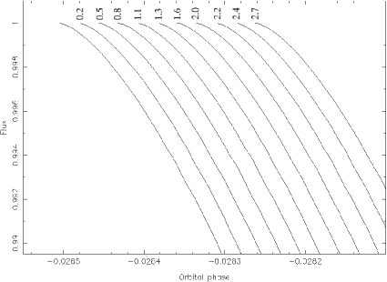
Figure 2: A sequence of simulated light curves around the time of white dwarf ingress. The eclipse assuming an immaculate photosphere is shown on the left. The other light curves assume that a Wilson–depressed starspot lies on the occulting limb and the depth of this depression is increased in 100 km steps from left to right. The time resolution of the light curves are all 0.1 seconds and the flux has been normalised by the out-of-eclipse contribution from the white dwarf. The ingress delay in seconds for each case, as measured against the immaculate photosphere model, is indicated above the corresponding light curve ingress point.

Figure 3: The difference, during ingress, between the immaculate eclipse light curve and the spotted eclipse light curve. The depth of the Wilson depression varies from 1000 km (top) to 100 km (bottom) in steps of 100 km.

Figure 4: A summary of how starspots of different Wilson depressions affect both the ingress delay (horizontal axis) and the maximum difference in flux between the ingress light curve of a spotted and immaculate star (vertical axis). The solid lines show the effects at different inclinations and the dashed lines indicate the depth of the Wilson depression assumed in each model.

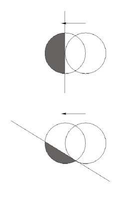
Figure 5: A schematic showing how the projected area of the white dwarf obscured per unit time is smaller for eclipsing systems of lower inclinations. The vertical line represent the limb of the occulting star and the circles represent the white dwarf. The top diagram depicts the white dwarf as it first contacts the companion (right-hand circle) in a high inclination binary. The left-hand circle depicts the white dwarf a short time later when the shaded portion has been eclipsed. The bottom panel shows the same scenario but for a lower inclination system. The arrow indicates the motion of the white–dwarf relative to the occulting limb of the red dwarf which has been depicted as stationary for clarity.

4 Observational practices

Given that starspots can alter the times of eclipse ingress and egress, it is important to understand the effect that this has on period determination and O–C analysis.

In order to investigate this we have used the model described in Sections 2 & 3 to simulate a series of eclipse light curves over many cycles. We assume a series of 12 hour long observations, each separated by a 30 day gap and all having a time resolution of 0.1 seconds. Over the 30 day interval between each 12 hour observation it is assumed that the spots evolve such that they are located in completely different positions. The spot distribution is modelled as a series of randomly placed spots of 30$\degr$ diameter covering a total of 30$\%$ of the stellar surface. Each spot is then randomly assigned a Wilson depression of between 100–1000 kilometres, leading to a systematic shift of the ingress or egress transition of 0.0–2.7 seconds. During the course of each 12 hour observation both the spot locations and depths are fixed. We adopt the binary parameters listed in Table LABEL:tab:pars throughout the simulations.

To investigate the effects of starspots, we first determined the time of mid–eclipse for each light curve by locating the start time of ingress and the end time of egress for each eclipse in turn. The mid–eclipse was then defined as lying exactly half–way between these points. We then fit these times of mid–eclipse over the whole set of simulated observations by a linear ephemeris of the form

$$HJD=T_{0}+nP,$$

where $T_{0}$ is the mid–eclipse zero–point, $n$ is the cycle number and $P$ is the orbital period. Fig. 6 shows the O–C diagram derived from this simulation. This shows that the presence of starspots causes a random ‘jitter’ in the O–C diagram. From Fig. 6 it is possible to distinguish between starspots that lie on the leading or trailing limb since a positive O–C residual results when a spot is on the leading limb, whereas a spot on the trailing limb results in a negative O–C residual. Where starspots lie on both limbs the O–C residual is dependent on which spot has the largest Wilson depression and hence it is more difficult to tell from Fig. 6 when this latter situation has occurred.

One might expect a correlation, however, between the eclipse duration (measured from the start of ingress to the end of egress and plotted in Fig. 7) and the observed O–C residuals. This is because the presence of a starspot on the leading limb of the occulting star will cause a delay in the ingress transition of, for example, $\delta t$ seconds. This would then cause the observed eclipse duration $D$ to shorten by $\delta t$ seconds but result in a smaller shift in the mid–eclipse timing of $\delta t/2$ seconds. If the precise orbital period and zero–point were known then the shift in the mid–eclipse timing would also result in an O–C residual of magnitude $\delta t/2$. Therefore, by plotting

$$D+2\times|O-C|,$$

points taken from observations where a spot lies on just one limb of the occulting star should fall on the same line, this is shown in Fig. 8. In practice, we do not know the precise period and zero–point, leading to the larger scatter seen in Fig. 8. Points where starspots are present on both limbs, however, lie systematically lower since their O–C residuals are partially cancelled out. Using this method, it is therefore also possible to identify those observations where starspots lie on both limbs.

Figure 6: The O–C diagram derived from the simulation described in Section 4. The left–pointing arrows denote observations where a spot lies on the trailing limb, right–pointing arrows denote observations when a spot lies on the leading limb, open circles where spots lie on both limbs and crosses where both limbs are clear of spots. Note that 3–4 eclipses are covered in each 12 hour observation, which leads to the grouping of several points around the same cycle number, the scatter in each group being due to timing errors assumed in the simulation.

Figure 7: The duration of each eclipse in seconds; the symbols are the same as in Fig 6.

Figure 8: A plot of the eclipse duration $D$ summed with twice the magnitude of the O–C residuals for that eclipse observation; The symbols are the same as in Fig 6.

Since we have shown how depressed starspots can affect O–C diagrams, we now investigate the impact that this has on the accuracy of both the period and the mid–eclipse zero-point ($T_{0}$) determined from the linear ephemeris fit. To do this we fit a linear ephemeris to the accumulated data after each observation date – essentially updating the ephemeris after each observation. We then compared the calculated period and mid–eclipse zero–point to the true values used in the simulation in order to asses how accurate the calculated values are, and how they vary with increasing cycle number. This information is shown in the left–hand panel of Fig. 9. The right–hand panel shows a similar analysis but for an immaculate star with no starspots as a comparison.

As can be seen, the orbital period is quickly determined to better than 1-ms accuracy after four separate observations (after cycle 695), even though some ingress and egress times are affected by the presence of starspots during this time. The reason why spots do not appear to have an adverse effect on the orbital period determination is that they only introduce a scatter in the O–C diagram (Fig. 6) and do not change its overall slope – allowing the orbital period to still be accurately determined.

The mid-eclipse zero-point ($T_{0}$) can also be determined with reasonable accuracy, although it still shows a departure from the true zero-point of $\sim$0.13 seconds after $\sim$11000 cycles. Another feature to note is that the trend in the mid-eclipse zero–point error appears to reflect that of the error in the orbital period. This is because a calculated orbital period that is longer than the true period causes the calculated times of mid–eclipse to become stretched out. This leads to the determination of an earlier zero–point in order to compensate for this and minimise the O–C residuals. It is this that causes the non–spotted O–C residuals in Fig. 6 to lie systematically below zero.

It should be noted that, although the overall slope of the O–C residuals is not changed by the presence of spots, during the appearance and/or disappearance of a starspot the slope of the O–C curve is temporarily changed. Therefore, spurious orbital period changes may be observed, especially over short time baselines. Indeed, a quadratic ephemeris fit did reveal a spurious but statistically significant orbital period change. Fit over the entire 1500 day dataset, we find that the rate of orbital change $\dot{P}$ = $9.5\times 10^{-9}\pm 1.0\times 10^{-9}$. In the model simulations presented here, this amounts to the false detection of a 1.2 second change in the orbital period over a four year interval. As a further check, we also produced a simulated dataset using a similar model to before but assuming zero starspot coverage. As expected, a quadratic ephemeris fit to this data did not find a significant period change.

Given that the appearance and disappearance of starspots on the limb is a largely random event (although there is evidence that starspots can form at preferred longitudes, see e.g. Holzwarth & Schüssler 2003), the sense and magnitude of the resultant $\dot{P}$ is also random. It would, therefore, be distinguishable from other mechanisms such as the Applegate effect (Applegate, 1992) and presence of a third body which both produce cyclical variations (e.g. Soydugan et al. 2003), and magnetic braking which will give a steadily decreasing orbital period. The orbital period change caused by the latter effect would also be reinforced by the parabolic dependence with time exhibited by a true orbital period change. In conclusion, the orbital period can still be accurately determined if the observations are carried out over a long enough interval over which the random effects of starspots will cancel out.

Figure 9: The discrepancy between the true orbital period and zero–point and those computed using a linear ephemeris fit. Top panel – the full line indicates the error (true - computed) on the orbital period, and the dashed lines indicates the error on the zero-point determination, both in seconds. Bottom panel – the error on the orbital period determination in milli-seconds. The left-hand panels show the results for the spotted model described in Section 4. and the right-hand panels show the results for an unspotted but otherwise identical model for comparison. It is clear that the orbital period can still be accurately determined within $\sim$ 3000 cycles despite the influence of starspots. The error in the zero–point is found to be greater, but is still determined to within $\sim$0.13 seconds over the full dataset.

5 Conclusions

In Section 3 we showed that depressed starspots can delay ingress or advance egress in eclipsing main-sequence white-dwarf binaries by several seconds, and that the magnitude of this effect becomes stronger for lower inclinations. We have also shown that it is, in principle at least, possible to determine both the inclination of the system and the depth of the Wilson depression from light curve analysis.

Depressed starspots also cause a ‘jitter’ in the residuals of O–C diagrams, which can also result in the false detection of spurious orbital period changes. Such changes due to starspots would be distinguishable from other mechanisms that cause period changes, and it should still be possible to determine the orbital period accurately.

Observational evidence for such effects are of interest. First, it would confirm that starspots also show the Wilson depression exhibited by sunspots – providing further tests of the solar-stellar connection. Second, it is not entirely clear whether the giant starspots that are found in Doppler images of rapidly rotating stars are actually monolithic, or groups of far smaller, individually unresolved, starspots. The effects described here will only be produced by relatively large starspots, and observations of these effects provide one of the few ways in which it would be possible to determine the monolithic nature (or otherwise) of starspots.

The best candidates in which to see the effects of Wilson–depressed starspots are eclipsing detached white–dwarf/late M–dwarf binaries, where the Applegate mechanism will be weak. However, even where the Applegate mechanism is strong, Wilson–depressed starspots would still cause variations in the eclipse width to be seen, which would otherwise remain constant under simple period changes.

Finally, Kalimeris et al. (2002) have shown that intensity variations due to starspots (not taking into account Wilson depressions) can introduce disturbances of up to $\sim$0.01 days in the O–C residuals of contact binaries. Given the rapid evolutionary timescales of spots (of the order of days) seen in recent Doppler images of the contact binary AE Phe (Barnes et al. 2004), this may lead to explaining some of the observed jitter in the O–C curves of these objects. Since, in this work, the effects of a Wilson depression seem to result in a scatter of only a few seconds in the O–C residuals, it seems unlikely that the Wilson depression will be a significant source of jitter for contact binaries. However, given the different geometries involved and procedures for determining standard time-markers, a proper assessment of whether this latter statement holds true is beyond the scope of this paper.

References

- Applegate (1992) Applegate J. H., 1992, ApJ, 385, 621
- Bagare & Gupta (1998) Bagare S. P., Gupta S. S., 1998, Bull. Astr. Soc. India, 26, 197
- Balthasar & Wohl (1983) Balthasar H., Wohl H., 1983, Solar Phys., 88, 71
- Barnes et al. (2004) Barnes J. R., Lister T., Hilditch R., Collier Cameron A., 2004, MNRAS, in press
- Catalán et al. (1994) Catalán M. S., Davey S. C., Sarna M. J., Smith R. C., Wood J. H., 1994, MNRAS, 269, 879
- Dhillon & Marsh (2001) Dhillon V. S., Marsh T. R., 2001, New Astron. Rev., 45, 91
- Dhillon & Marsh (2004) Dhillon V. S., Marsh T. R., 2004, MNRAS, in preparation
- Hendry & Mochnacki (2000) Hendry P. D., Mochnacki S. W., 2000, ApJ, 531, 467
- Holzwarth & Schüssler (2003) Holzwarth V., Schüssler M., 2003, A&A, 405, 303
- Kalimeris et al. (2002) Kalimeris A., Rovithis-Livaniou H., Rovithis P., 2002, A&A, 387, 969
- Marsh (2004) Marsh T. R., 2004, private communication
- O’Neal et al. (1998) O’Neal D., Saar S. H., Neff J. E., 1998, ApJ, 501, L73
- Rajaguru & Hasan (2002) Rajaguru S. P., Hasan S. S., 2002, in Strassmeier K. G., Washuettl A., eds, 1st Potsdam Thinkshop on Sunspots and Starspots AIP, p. 115
- Ramseyer et al. (1995) Ramseyer T. F., Hatzes A. P., Jablonski F., 1995, AJ, 110, 1364
- Soydugan et al. (2003) Soydugan F., Demircan O., Soydugan E., İbanoğlu C., 2003, AJ, 126, 393
- Suzuki (1967) Suzuki Y., 1967, PASJ, 19, 220