Cross section predictions for hydrostatic and explosive burning

Abstract

We review different models used for reactions involved in nuclear astrophysics. The reaction rate is defined for resonant as well as for non-resonant processes. For low-density nuclei, we describe the DWBA method, the potential model, the $R$-matrix method, and microscopic cluster models. The statistical model is developed for high-level densities. Details of calculations in the low- and high-density regimes are illustrated with new results concerning transfer reactions and level densities.

and

1 Introduction

Nuclear reactions are important for studying energy generation and nucleosynthesis in astrophysical processes [1, 2]. Especially in explosive burning scenarios, large reaction networks include mainly nuclei far from stability which have not been studied experimentally so far, and perhaps will never be accessible in the laboratory. This poses a challenge to both experimentalists and especially theorists, which have to predict reaction cross sections of more or less unknown nuclei. Another challenge is found in the comparatively low interaction energies which pose problems for predictions as well as for measurements already close to and at stability. Here we provide and overview of the current status of theory and details of the remaining challenges, illustrated by several examples of new calculations.

Theoretical models can be roughly classified in three categories [3]:
$(i)$ Models involving adjustable parameters, such as the $R$-matrix [4] or the $K$-matrix [5] methods; parameters are fitted to the available experimental data and the cross sections are extrapolated down to astrophysical energies. These fitting procedures of course require the knowledge of data, which are sometimes too scarce for a reliable extrapolation.
$(ii)$ “Ab initio” models, where the cross sections are determined from the wave functions of the system. The potential model [6], the Distorted Wave Born Approximation (DWBA) [7], and microscopic models [8, 9] are, in principle, independent of experimental data. More realistically, these models depend on some physical parameters, such as a nucleus-nucleus or a nucleon-nucleon interaction which can be reasonably determined from experiment only. The microscopic Generator Coordinate Method (GCM) provides a “basic” description of a $A$-nucleon system, since the whole information is obtained from a nucleon-nucleon interaction. Since this interaction is nearly the same for all light nuclei, the predictive power of the GCM is important.
$(iii)$ Models $(i)$ and $(ii)$ can be used for low level-density nuclei only. This condition is fulfilled in most of the reactions involving light nuclei ($A\leq 20$). However when the level density near threshold is large (i.e. more than a few levels per MeV), statistical models, using averaged optical transmission coefficients, are more suitable (see Sec. 4).

In Sec. 2, we start with useful definitions commonly used in nuclear astrophysics, such as of the reaction rates which are the actual quantities used in reaction networks, and their relation to cross sections and the relevant energy range. We then discuss different approaches and reaction mechanisms for systems with low (Sec. 3) and high level densities (Sec. 4). In nuclear astrophysics, the relevant projectile energy range often covers both the low and high density regimes. The difficulties concerning the prediction of reaction rates bridging the two regimes are briefly addressed in Sec. 4.3. Concluding remarks are presented in Sec. 5.

2 Reaction Rates

Let us consider a reaction between two nuclei with masses $A_{1}m_{N}$ and $A_{2}m_{N}$ and charges $Z_{1}e$ and $Z_{2}e$ (we express here the masses in units of the nuclear mass $m_{N}$). The theory of stellar evolution involves the reaction rate at temperature $T$, defined as [10, 1, 2]

$$N_{A}<\sigma v> = N_{A}\left(\frac{8}{\pi\mu m_{N}(k_{B}T)^{3}}\right)^{\frac{1}{2}}\ \int\sigma(E)\,E\,\exp(-E/k_{B}T)\,dE,$$ (1)

where we assume that the star can be considered as a perfect gas following the Maxwell-Boltzmann distribution. In Eq. (1), $v$ is the relative velocity, $N_{A}$ is Avogadro’s number, $\mu$ is the dimensionless reduced mass, and $k_{B}$ is Boltzmann’s constant. At sub-coulomb energies the cross section varies as

$$\sigma(E)\sim\exp(-2\pi\eta)/E,$$ (2)

where $\eta=Z_{1}Z_{2}e^{2}/\hbar v$ is the Sommerfeld parameter.

Using (2), the integrand of (1) can be approximated by a Gaussian shape [10, 1] with a maximum at the Gamow peak. The energy and width are given by

$$E_{0}=\left[\pi\frac{e^{2}}{\hbar c}Z_{1}Z_{2}k_{B}T(\mu m_{N}c^{2}/2)^{1/2}\right]^{2/3}\approx 0.122\,\mu^{1/3}(Z_{1}Z_{2}T_{9})^{2/3}\ {\rm MeV},$$ (3)

$$\Delta E_{0}=4(E_{0}k_{B}T/3)^{\frac{1}{2}}\approx 0.237\,(Z_{1}^{2}Z_{2}^{2}\mu)^{1/6}\,T_{9}^{5/6}\ {\rm MeV},$$ (4)

where $T_{9}$ is the temperature expressed in $10^{9}K$. The Gamow energy defines the energy range where the cross section needs to be known to derive the reaction rate. In most cases, this energy is much lower than the Coulomb barrier which means that the cross sections drop to very low values. To compensate the fast energy dependence of the cross section, nuclear astrophysicists use the $S$-factor defined as

$$S(E)=\sigma(E)\,E\,\exp(2\pi\eta),$$ (5)

which is mainly sensitive to the nuclear contribution of the cross section. For non-resonant reactions, the energy dependence of the $S$ factor is smooth.

Rigorously the reaction rate should be calculated numerically by using experimental or theoretical cross sections. However, the analytical approach provides a more intuitive understanding of the physics, and is still widely used. Let us start with non-resonant reactions, where the $S$-factor weakly depends on energy. In this case, the integral (1) can be replaced by an accurate analytical approximation. A Taylor expansion near $E_{0}$ provides

$$\exp(-2\pi\eta-E/k_{B}T)\approx\exp(-3E_{0}/k_{B}T)\exp\left(-\left(\frac{E-E_{0}}{\Delta E_{0}/2}\right)^{2}\right).$$ (6)

Assuming a linear variation of $S(E)$ in the Gamow peak [1], the reaction rate is then given by

$$N_{A}<\sigma v> \approx N_{A}\left(\frac{32E_{0}}{3\mu m_{N}(k_{B}T)^{3}}\right)^{\frac{1}{2}}\exp\left(-\frac{3E_{0}}{k_{B}T}\right)\,\left(1+\frac{5k_{B}T}{36E_{0}}\right)$$ (7)

$$\times S(E_{0}+\frac{5}{6}k_{B}T),$$

which presents a fast variation with temperature.

The formalism developed here is valid for any form of the $S$-factor. The analytical procedure can be extended further by assuming a quadratic form of the $S$-factor

$$S(E)\approx S_{0}+S^{\prime}_{0}E+\frac{1}{2}S^{\prime\prime}_{0}E^{2},$$ (8)

which is used in some astrophysics tables [10]. We have

$$N_{A}<\sigma v>\approx N_{A}\left(\frac{32E_{0}}{3\mu m_{N}(k_{B}T)^{3}}\right)^{\frac{1}{2}}\exp\left(-\frac{3E_{0}}{k_{B}T}\right)$$

$$\times\left[S_{0}(1+\frac{5k_{B}T}{36E_{0}})+S^{\prime}_{0}(E_{0}+\frac{35}{36}k_{B}T)+\frac{1}{2}S^{\prime\prime}_{0}E_{0}(E_{0}+\frac{89}{36}k_{B}T)\right].$$ (9)

This yields the well known $T^{1/3}$ expansion of the reaction rate, up to $T^{5/3}$ [10]; Eq.(9) provides the rate from the $S$-factor properties at zero energy.

For resonant reactions, the $S$-factor is assumed to have a Breit-Wigner form (for the Breit-Wigner expression for cross sections see Eq. 31). The general definition (1) is of course still valid. However, one has to account for the fast variation of $S(E)$ near the resonance energy. Since a numerical approach is difficult for narrow resonances, we present an analytical method, widely used in nuclear astrophysics.

A careful analysis of integrand (1) shows that it always presents two maxima: at the resonance energy, and at the Gamow energy. The peak at the resonance energy does not depend on temperature. The second peak, corresponding to the Gamow energy, moves according to the temperature. From these considerations, and except in the temperature range where both peaks overlap, the resonant reaction rate can be split in two terms

$$N_{A}<\sigma v>\approx N_{A}<\sigma v>_{R}\,+\,N_{A}<\sigma v>_{T},$$ (10)

where $N_{A}<\sigma v>_{R}$ corresponds to the maximum at $E=E_{R}$. For a narrow resonance, we have

$$N_{A}<\sigma v>_{R}=N_{A}\left(\frac{2\pi}{\mu m_{N}k_{B}T}\right)^{\frac{3}{2}}\hbar^{2}\omega\gamma\exp(-E_{R}/k_{B}T),$$ (11)

where the resonance strength $\omega\gamma$ is defined by

$$\omega\gamma=\frac{2J+1}{(2I_{1}+1)(2I_{2}+1)}\,\frac{\Gamma_{1}\Gamma_{2}}{\Gamma_{1}+\Gamma_{2}},$$ (12)

$J$ being the spin of the resonance, and ($\Gamma_{1},\Gamma_{2}$) the widths in the entrance and exit channels. In capture reactions, the $\gamma$ width is in general much lower than the particle width. The resonance strength is then proportional to the lower partial width.

The second maximum of integrand (1) yields the so-called ”tail resonance” term $N_{A}<\sigma v>_{T}$. Its analytical expression is identical to the non-resonant rate (7) with a Breit-Wigner expression for $S(E)$.

3 Systems with low level densities

3.1 Introduction

Although it is in general not trivial to draw a distinct line between the direct and the compound reaction mechanism (as, e.g., in the case of processes involving only few interaction steps of a few nucleons without participation of the bulk of nucleons), direct reactions are usually assumed to be fast, one-step processes with few degrees of freedom in which the captured particle directly enters the final state without sharing any energy with other nucleons [11]. It has long been known that direct reactions mainly occur at high projectile energies where the formation of a compound nucleus is suppressed due to the slow reaction time-scale [11, 12]. Such high projectile energies ($E_{\mathrm{proj}}\gtrsim 20$ MeV) are not important in the effective energy range relevant for hydrostatic or explosive astrophysical burning. However, direct reactions can also dominate the cross section at very low energies in systems with low level densities. This occurs for light nuclei and for nuclei with low particle separation energies. For example, very neutron-rich nuclei far off stability have decreasing neutron separation energies which implies that low level densities are encountered in the projectile-target system at $r$-process energies. Similar considerations hold for proton-rich nuclei close to the proton dripline encountered in the $rp$-process. A special case concerns nuclei with magic nucleon numbers. Due to their wide level spacing, direct reactions may become important for intermediate and heavy nuclei already close to or at the line of stability (see also Sec. 4.2). On the other hand, reactions in light nuclei are always direct because the reaction systems contain only few nucleons. Due to this fact, reactions in solar burning have been known to proceed via the direct mechanisms since decades. More recently, a number of studies have analyzed reactions in astrophysical burning (for both capture and transfer reactions) and also investigated direct interactions in neutron capture on intermediate and heavy nuclei far off stability occurring in the $r$-process [13, 14, 15, 16, 17].

In fact, the distinction between direct and compound reactions might be misleading, especially in light nuclei. For example, it is often assumed that the term “direct” is synonymous to “non-resonant”. This is incorrect since potential resonances can still be included in the models described below (e.g. [13]). Only very narrow single-particle resonances are not reproduced in models using effective optical potentials. Therefore we prefer to address reactions in low level density systems and such in systems with high level densities, and to present the relevant models for cross section predictions in this context. Nevertheless, for simplicity we will still occasionally use the term “direct” in the following discussion. However, it is to be understood as described above.

The discussion of reactions in low level-density systems is started with distorted wave methods for transfer and capture reactions, belonging to the group of potential models which describe the dynamics of a system by solving the Schrödinger equation with an effective potential. The potential is of optical-potential type (see also Sec. 4.1) but other nucleus-nucleus potentials are used in different models due to the nature of the model and varying approximations of coupling to other channels [11].

3.2 The DWBA method for transfer reactions

The Distorted Wave Born Approximation (DWBA) starts from the premise that elastic scattering is dominant and has to be treated fully, while non-elastic events can be treated by perturbation theory. Although DWBA is a first-order theory, the way it is usually applied is not simply first-order. That is because optical potentials fitted to elastic scattering data may include higher-order effects implicitly. Therefore different potentials are needed for higher-order methods, such as coupled-channels calculations, than those used in DWBA in order to reproduce the same elastic data.

The DWBA method can be applied to transfer reactions

$$a(=b+x)+A\rightarrow b+B\,(=A+x)$$ (13)

and assumes that particle $x$ goes from the projectile $a$ to the target $A$ [11]. The cross section for reaction (13) is obtained from the matrix elements

$$T^{\rm DWBA}=\int\int d\mbox{$\mbox{\boldmath$\rho$}$}_{\alpha}d\mbox{$\mbox{\boldmath$\rho$}$}_{\beta}\,\chi^{-}_{\beta}(\mbox{$\mbox{\boldmath$\rho$}$}_{\beta})<\Psi_{b}\Psi_{B}|\Delta V|\Psi_{a}\Psi_{A}>\chi^{+}_{\alpha}(\mbox{$\mbox{\boldmath$\rho$}$}_{\alpha}),$$ (14)

where the distorted waves $\chi^{+}_{\alpha}(\mbox{$\mbox{\boldmath$\rho$}$}_{\alpha})$ and $\chi^{-}_{\beta}(\mbox{$\mbox{\boldmath$\rho$}$}_{\beta})$, ($\mbox{$\mbox{\boldmath$\rho$}$}_{\alpha}$ and $\mbox{$\mbox{\boldmath$\rho$}$}_{\beta}$ are the relative coordinates) corresponding to the relative motion in the entrance and exit channels, respectively, are generated by optical potentials $U_{\alpha}$ and $U_{\beta}$. The residual interaction is defined in two different ways

$$\Delta V = V_{xA}+V_{bA}-U_{\alpha}\rm{\ \ (prior)}$$ (15)

$$= V_{bx}+V_{bA}-U_{\beta}\rm{\ \ (post)},$$

which correspond to ”prior” and ”post” definitions, respectively; they provide identical values for $T^{DWBA}$. The main problem of the method is that the potentials are usually poorly known. In general, a good approximation is to neglect $V_{bA}-U_{\alpha}$ or $V_{bA}-U_{\beta}$. The matrix element then contains distorted scattering wave functions $\chi_{\alpha}$, $\chi_{\beta}$, and the radial bound state wave functions of the transferred cluster. All of these wave functions are usually numerically computed with optical potentials as shown in Sec. 4.1.

Since more realistic descriptions of nucleus $a(B)$ should involve other configurations than $b+x\ (A+x)$, spectroscopic factors are introduced ($\mathcal{S}_{a}$ and $\mathcal{S}_{B}$). The DWBA cross section is therefore linked to the experimental cross section through

$$\sigma_{\rm exp}=\mathcal{S}_{a}\,\mathcal{S}_{B}\,\sigma_{\rm DWBA}.$$ (16)

A recent work [18] aims at investigating the precision of the DWBA for transfer reactions at low energies. We have investigated the ¹³C($\alpha$,n)¹⁶O reaction by a microscopic model, and used the DWBA in conditions as close as possible to the reference calculation. The conclusion is twofold. On one hand, the DWBA method turns out to be very sensitive to the conditions of the calculations: choice of the nucleus-nucleus potentials and, to a lesser extent, of the internal wave functions of the colliding nuclei. This sensitivity is due to very basic properties, i.e. the short-range character of the DWBA matrix elements, which are quite sensitive to details of the wave functions. On the other hand, the difference between the DWBA and the reference microscopic method can be fairly large, and varies with angular momentum. This is most likely due to antisymmetrization effects which are approximately included in the DWBA through the choice of deep nucleus-nucleus potentials. This property should also occur in other systems and suggests that the DWBA method can only provide transfer cross sections with a non-negligible uncertainty.

Future experiments with unstable beams will provide valuable information on the level structure and spectroscopic factors (also for the important neutron capture reactions discussed in Sec. 3.3). Usually, (d,p) reactions are used for this purpose as neutron capture at low energies cannot be studied on radioactive isotopes. However, an analysis of the results might be complicated because the experimental cross sections have to be compared to calculations which still bear considerable uncertainties in the optical potentials used. One has to be extremely cautious in interpreting such comparisons as the resulting spectroscopic factors may carry large uncertainties. A promising way out might be the use of the adiabatic approximation instead of DWBA which arises from neglecting the internal excitation energies of states relative to the bombarding energy [11, 19]. It can be formulated in such a manner that no optical potentials are needed [20]. Some parameters have to be adjusted by including elastic data but no further reaction information is required. Further investigation will show whether this approach is practicable for reactions far off stability.

3.3 Capture reactions in a potential model

Capture reactions can be treated in a first-order approach involving an electromagnetic operator describing the emission of $\gamma$-radiation due to the dynamics in the movement of the electric charges. Since the application to neutron or proton capture dominated by electric dipole transitions is most important in astrophysics, here we give the expression for E1 direct capture. The cross section of the direct radiative capture process $a+A\rightarrow\gamma+B$, which is entirely electromagnetic, is given by [2, 21, 22]:

$$\sigma_{\rm E1} = \frac{16\pi}{9}\left(\frac{E_{\gamma}}{\hbar c}\right)^{3}\frac{e^{2}\mu_{\alpha}^{3}}{\hbar^{2}k_{\alpha}}\frac{3}{\left(2I_{\rm a}+1\right)\left(2I_{\rm A}+1\right)}\left(\frac{Z_{\rm a}}{m_{\rm a}}-\frac{Z_{\rm A}}{m_{\rm A}}\right)^{2}C^{2}\mathcal{S}_{\ell_{\beta}J_{\beta}}$$ (20)

$$\times\sum_{\ell_{\alpha}J_{\alpha}}\left(2J_{\beta}+1\right)\left(2J_{\alpha}+1\right)\max\left(\ell_{\alpha},\ell_{\beta}\right)$$

$$\times\left\{\begin{array}[]{ccc}1&\ell_{\beta}&\ell_{\alpha}\\ I&J_{\alpha}&J_{\beta}\end{array}\right\}^{2}a_{I}^{2}\left|R_{1\beta\alpha}\right|^{2}$$

with the radial integral

$$R_{1\beta\alpha}=\frac{1}{k_{\alpha}}\int u_{\beta}^{*}(r)\chi_{\alpha}(r)\;r\;dr\quad.$$ (21)

In the above expression, the energy of the emitted photon is $E_{\gamma}$. The charge and mass of the projectile and target nucleus are $Z_{\rm a}$, $m_{\rm a}$, $Z_{\rm A}$ and $m_{\rm A}$, respectively. The orbital and total angular momentum quantum numbers of the nuclei in the entrance and exit channels are $\ell_{\alpha}$, $J_{\alpha}$, $\ell_{\beta}$ and $J_{\beta}$, respectively. The spin quantum number, the orbital and total angular momentum quantum numbers are characterized by $S$, $L$ and $I$, respectively, with indices a, A and B corresponding to the projectile, target and residual nucleus, respectively. The symbol $\left\{\matrix{\ldots}\right\}$ is the $6j$ symbol. The radial distorted wave in the entrance channels is given by $\chi_{\alpha}$. The radial bound state wave function of the final state is denoted by $u_{\beta}$. The spectroscopic factor and the isospin Clebsch–Gordan coefficient for the partition $B=A+a$ are given by $C$ and ${\mathcal{S}}_{\ell_{\beta}J_{\beta}}$, respectively.

The required wave functions $\chi_{\alpha}$, $u_{\beta}$ are found by solving the Schrödinger equation with an appropriate optical potential. The spectroscopic factor is the overlap of the wavefunctions of the target and the final nucleus and is extracted from experiment or a more microscopic calculation. In case of single nucleon capture the spectroscopic factor is simply related to the occupation probability $V^{2}$ of the orbital into which the nucleon is captured, e.g., ${\mathcal{S}}=(1-V^{2}_{j})$ for depositing a nucleon onto an even target [12]. The same spectroscopic factor applies to (d,p) and (d,n) reactions, respectively. For a discussion of how to extract spectroscopic factors for neutron or proton capture such transfer reactions, see the end of the previous Sec. 3.2.

The optical potential can be derived using the folding approach (see Sec. 4.1) and by determining the parameter $\lambda$ from systematics of volume integrals [23]. The capture cross sections are very sensitive to excitation energy and spin of the final states. This poses a big problem far off stability where there is no experimental information available. It has been shown that neutron capture cross sections predicted utilizing input from different microscopic structure models can differ by orders of magnitude [24]. Large jumps in the cross section when going along an isotopic chain were also found, due to the fact that a weakly bound state (which nevertheless dominates the cross section) can become unbound in the subsequent isotope and become unavailable for capture.

3.4 R-matrix

In the $R$-matrix method, the energy dependence of the cross sections is obtained from Coulomb functions, as expected from the Schrödinger equation. The goal of the $R$-matrix method [4] is to parameterize some experimentally known quantities, such as cross sections or phase shifts, with a small number of parameters, which are then used to extrapolate the cross section down to astrophysical energies.

The $R$-matrix framework assumes that the space is divided into two regions: the internal region (with radius $a$), where the nuclear force is important, and the external region, where the interaction between the nuclei is governed by the Coulomb force only. Although the $R$-matrix parameters do depend on the channel radius $a$, the sensitivity of the cross section with respect to its choice is quite weak. The physics of the internal region is parameterized by a number $N$ of poles, which are characterized by energy $E_{\lambda}$ and reduced widths $\gamma_{\lambda\alpha}$. In a multichannel problem, the $R$-matrix at energy $E$ is defined as

$$R_{\alpha\beta}(E)=\sum_{\lambda=1}^{N}\frac{\gamma_{\lambda\alpha}\gamma_{\lambda\beta}}{E_{\lambda}-E},$$ (22)

which must be given for each partial wave $J$. Indices $\alpha$ and $\beta$ refer to the channels.

The $R$-matrix method can be applied to transfer as well as to capture reactions. It is usually used to investigate resonant reactions but is also suited to describe non-resonant processes [25]. In the latter case, the non-resonant behavior is simulated by a high-energy pole, referred to as the background contribution, which makes the $R$-matrix nearly energy independent. The pole properties are associated with the physical energy and width of resonances, but not strictly equal. This is known as the difference between “formal” parameters and “observed” parameters, deduced from experiment. In a general case, involving more than one pole, the link between those two sets is not straightforward; recent works [26, 27] have established a general formulation to deal with this problem.

Figure 1 shows a recent application to the ¹⁴N(p,$\gamma)^{15}$O reaction (ground-state contribution) with the data obtained by the LUNA collaboration [28] . Within the $E1$ multipolarity, $1/2^{+}$ and $3/2^{+}$ resonances are taken into account. The ground-state contribution represents about 15% of the total $S$ factor. At zero energy, we have $S(0)=1.7\pm 0.2$ keV-b, in agreement with previous results.

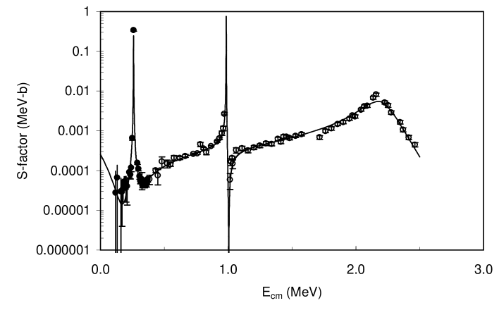
Figure 1: $R$-matrix fit of the ¹⁴N(p,$\gamma$)¹⁵O reaction for capture to the ¹⁵O ground-state. Open circles are the data of Schröder et al. [29] and full circles represent the LUNA data [28].

3.5 Microscopic models

Microscopic models are based on basic principles of quantum mechanics, such as the treatment of all nucleons, with exact antisymmetrization of the wave functions. The hamiltonian of an $A$-nucleon system is

$$H=\sum^{A}_{i=1}T_{i}\ +\ \sum^{A}_{i<j=1}V_{ij},$$ (23)

where $T_{i}$ is the kinetic energy and $V_{ij}$ a nucleon-nucleon interaction [8, 9].

The Schrödinger equation associated with this hamiltonian can not be solved exactly when $A>3$. The Quantum Monte Carlo method [30] represents a significant breakthrough in this direction, but is currently limited to $A=10$. In addition its application to continuum states is not feasible for the moment (it has been applied to the d$(\alpha,\gamma)^{6}$Li reaction [31], but the $\alpha+d$ relative motion is described by a nucleus-nucleus potential).

In cluster models, it is assumed that the nucleons are grouped in clusters. We present here the application to two-cluster systems. This provides a natural extension of the formalism to scattering states. The internal wave functions of the clusters are denoted as $\phi_{i}^{I_{i}\pi_{i}\nu_{i}}(\mbox{\boldmath$\xi_{i}$})$, where $I_{i}$ and $\pi_{i}$ are the spin and parity of cluster $i$, and $\xi_{i}$ represents a set of its internal coordinates. One defines the channel function as

$$\varphi^{JM\pi}_{\ell I}(\Omega_{\rho},\mbox{\boldmath$\xi_{1}$},\mbox{\boldmath$\xi_{2}$})=\left[Y_{\ell}(\Omega_{\rho})\otimes[\phi_{1}^{I_{1}\pi_{1}}(\mbox{\boldmath$\xi_{1}$})\otimes\phi_{2}^{I_{2}\pi_{2}}(\mbox{\boldmath$\xi_{2}$})]^{I}\right]^{JM},$$ (24)

where different quantum numbers show up: the channel spin $I$, the relative angular momentum $\ell$, the total spin $J$ and the total parity $\pi={\pi}_{1}{\pi}_{2}{(-)}^{\ell}$.

The total wave function is written as

$$\Psi^{JM\pi}=\sum_{\alpha\ell I}{\mathcal{A}}\,g^{J\pi}_{\alpha\ell I}(\rho)\ \varphi^{JM\pi}_{\alpha\ell I}(\Omega_{\rho},\mbox{\boldmath$\xi^{i}_{1}$},\mbox{\boldmath$\xi^{j}_{2}$}),$$ (25)

which corresponds to the Resonating Group (RGM) definition. Index $\alpha$ corresponds to different two-cluster arrangements, and $\mathcal{A}$ is the antisymetrization operator. In most applications, the internal cluster wave functions are defined in the shell model. Accordingly, the nucleon-nucleon interaction must be adapted to this choice, which leads to effective forces, such as the Volkov [32] or the Minnesota [33] interactions. The relative wave function $g(\rho)$ is to be determined from the Schrödinger equation. In recent applications, this function is expanded over gaussian functions [8, 34], which corresponds to the Generator Coordinate Method (GCM). The GCM is equivalent to the RGM, but is better adapted to numerical calculations, as it makes uses of projected Slater Determinants.

The main advantage of cluster models with respect to other microscopic theories is its ability to deal with reactions, as well as with nuclear spectroscopy. The first applications were done for reactions involving light nuclei, such as d, ³He or $\alpha$ particles. More recently, much work has been devoted to the improvement of the internal wave functions: multicluster descriptions [35, 36], large-basis shell model extensions [37], or monopolar distortion [38]. Microscopic cluster models have a wide range of applications, both in low-energy reactions and in the spectroscopy of light nuclei. The main limitation arises from the number of channels included in the wave function, which reduces the validity of the model at low energies. Also high-level densities require many channels in the wave functions. Nuclear astrophysics is probably one of the best candidates for applications of microscopic cluster models. The low energies and the low densities involved in most nuclei make the conditions of application quite valid.

We illustrate cluster models with a recent application to the ¹⁷F(p,$\gamma)^{18}$Ne reaction [39]. The knowledge of the ¹⁷F(p,$\gamma)^{18}$Ne reaction rate is important for the understanding of the energy production and of the nucleosynthesis in novae [40]. Until now, a direct measurement of the cross section down to astrophysical energies (typically 0.3 MeV) has not been performed. It is now well established that the $3^{+}_{1}$ level dominates the rate at high temperatures since it is the only $s-$wave resonance at low energies. The gamma width remains experimentally unknown and is estimated by shell-model calculations. At low temperatures, the non-resonant contribution is dominant but is evaluated with simple models [41] which need confirmation from more elaborate theories.

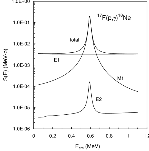
Figure 2: ¹⁷F(p,$\gamma)^{18}$Ne astrophysical $S$-factor with the contribution of different multipolarities.

The GCM wave functions are defined as a combination of ¹⁷F + p and $\alpha+^{14}$O channel functions. The ¹⁷F and the ¹⁴O nuclei are described by $s,p$ and $sd$ (for ¹⁷F) harmonic oscillator shells. This framework allows the description of the ¹⁷F$(5/2^{+},1/2^{+},3/2^{+})$+p and ¹⁴O$(0^{+},2^{+})+\alpha$ channels.

The proton width of the $3^{+}$ resonance (21 keV) is in fair agreement with the experimental value ($18\pm 3$ keV) [42]. For the gamma width, we find 33 meV; a recent evaluation of the reaction rate [42] uses $\Gamma_{\gamma}=29\pm 19$ meV. The astrophysical $S$-factor is calculated for the $E1$, $E2$, and $M1$ multipolarities. In each case, the four $0^{+}_{1}$,$2^{+}_{1}$, $2^{+}_{2}$ and $4^{+}_{1}$ bound states are considered. The $J$ values for scattering states are limited to 4, which corresponds to $\ell=2$. The total and partial $S$-factors are displayed in Fig. 2.

4 Systems with high level densities

4.1 Optical model

Due to the complexity of the nucleon-nucleon (NN) interaction, one often resorts to working with effective interactions instead of solving microscopic models based on NN potentials (but see Sec. 3.5). Widely used in calculating different reaction mechanisms is the optical model. In that model, the complicated many-body problem posed by the interaction of two nuclei is replaced by the much simpler problem of two particles interacting through an effective potential, the so-called optical potential [11, 12, 43]. Such an approach is usually feasible only with few contributing channels. Always included is elastic scattering. That is why optical potentials can be derived from elastic scattering data.

In general, the optical potential is complex. The real part describes the refraction of the incident waves by the nucleus (elastic scattering), the imaginary part their absorption, hence the term “optical” model. Thus, the imaginary part of the resulting wave function contains all non-elastic processes removing flux from the incident channel. In general, the potential is expected to be energy-dependent for obvious reasons. Most applications make use of local potentials although, in principle, also the effective potential should be non-local. An additional slight energy-dependence is introduced by this neglection [11].

The required potential parameters can be derived either by fits to experimental elastic data or from microscopic considerations. An example of the latter is the folding approach [44] which is often employed to determine the real potential. In this approach an effective NN interaction is folded with projectile and target nucleon density distributions. The latter have to be derived from electron scattering data or further microscopic considerations. Another example for a more microscopic approach is the use of the local density approximation [45, 46]. The advantage of this model is that also the imaginary part can be determined. Again, certain parameters have to be fitted to experimental data and density distributions have to be known.

The standard definition of the optical model stems from the description of elastic and inelastic scattering. The time-independent radial Schrödinger equation is numerically solved with an optical potential which provides a mean interaction potential, averaging over individual NN interactions. In consequence, single-particle resonances cannot be described in such a model. However, resonances stemming from potential scattering can still be found. Elementary scattering theory yields expressions for the elastic cross section and the reaction cross section. The latter includes all reactions and inelastic processes which cause loss of flux from the elastic channel. With the diagonal element $S^{\alpha\alpha}$ of the S-matrix $S$ (sometimes also called scattering matrix or collision matrix), the reaction cross section for spinless particles is then given by [43]

$$\sigma^{\alpha\alpha}_{\mathrm{r}}=\frac{\pi}{k^{2}}\sum_{L}\left(2L+1\right)\left(1-\left|S^{\alpha\alpha}_{L}\right|^{2}\right)\quad.$$ (26)

This can be generalized to other channels $\beta$, not just the elastic one. The elements of the S-matrix are complex, in general, and related to the scattering amplitude $f$ of the outgoing wave function

$$f^{\alpha\beta}=\frac{1}{2ik}\sum_{L}(2L+1)(S^{\alpha\beta}_{L}-1)P_{L}(\cos\theta)\quad,$$ (27)

which is nothing else than the transition amplitude $T^{\alpha\beta}=-(2\pi\hbar)/\mu_{\beta}f^{\alpha\beta}$, in turn, with $\mu$ being the reduced mass. As mentioned above, the imaginary part of the optical potential gives rise to an absorption term in the solution of the Schrödinger equation, thus removing flux from the considered channels. Therefore, the matrix element $S^{\alpha\alpha}$ is also related to the transmission coefficient

$$t_{L}=\left(1-\left|\mathrm{e}^{2i\delta_{L}}\right|^{2}\right)=1-\left|S^{\alpha\alpha}_{L}\right|^{2}$$ (28)

which describes the absorption of the projectile by the nucleus. Important for practical application is that the phase shifts $\delta_{L}$ can be derived from elastic data.

In the preceding Sec. 3.1 we have already discussed several models making use of potentials of the optical type. In the following, the statistical model of nuclear reactions is described which also applies optical potentials to calculate the formation and decay of the compound nucleus.

4.2 Statistical model

It is well established that the number of states in a nucleus increases in principle exponentially with excitation energy. Thus, with increasing projectile energy, different resonance regimes are covered. Starting without or only few resonances at low energy and more, but still well separated, resonances at intermediate energies, one will eventually encounter a region where the average resonance width $\left<\Gamma\right>$ becomes larger than the average level spacing $D=1/\rho$. This is the domain of the compound nucleus reaction which can be calculated in a statistical model only using average resonance properties, also called the Hauser-Feshbach approach. In astrophysical applications, the compound reaction mechanism is especially important for reactions with charged projectiles as the relevant energy range (given by the Gamow peak, eq. 4) is shifted to higher energies as compared to neutron-induced reactions. Nevertheless, also for reactions involving neutrons the statistical model can be applied when the reaction $Q$-value or the level density is sufficiently high. This is true for most intermediate and heavy nuclei close to stability with non-magic neutron numbers. The relevant quantity is the number of available levels in the Gamow peak. An estimate of the applicability range of the statistical model is given in [47].

The statistical model is based on the Bohr independence hypothesis [48]. It states that the projectile forms a compound system with the target and shares its energy among all of the nucleons. This implicitly requires long reaction time-scales as the compound nucleus has to live long enough to establish complete statistical equilibrium. Compared to the direct mechanism (Sec. 3.1) it is about 5 orders of magnitude longer and includes many degrees of freedom. Finally, the compound nucleus can decay by emitting photons or particles. According to the Bohr hypothesis the final decay is independent of the formation process, except for the basic conservation laws of energy, angular momentum, parity, and nucleon number. Thus, the cross section can be factorized into two terms

$$\sigma^{\alpha\beta}_{\mathrm{CN}}=\sigma^{\alpha}_{\mathrm{form}}b_{\mathrm{dec}}=\sigma^{\alpha}_{\mathrm{form}}\frac{\left<\Gamma^{\beta}\right>}{\left<\Gamma_{\mathrm{tot}}\right>}\quad.$$ (29)

the formation cross section $\sigma_{\mathrm{form}}$ and a branching ratio describing the probability for decay to the observed channel $\beta$. An early implementation of this was the Weisskopf-Ewing theory [49]. Today, the Hauser-Feshbach approach [50] is widely used which also incorporates angular momentum conservation. Modern theories also treat pre-equilibrium emission of particles in different ways. However, for the energies encountered in astrophysical scenarios, this additional mechanism is usually negligible.

In the Hauser-Feshbach theory, the formation cross section is calculated as in the optical model (Sec. 4.1) but using averaged transmission coefficients $\left<T\right>$ which can again be computed from a Schrödinger equation and using appropriate optical potentials. The average widths occurring in the branching ratio $b_{\mathrm{dec}}$ are related to average transmission coefficients via $\left<T\right>=2\pi\rho\left<\Gamma\right>$, with $\rho$ being the average level density. In fact, it can be shown [51] that the expression for the compound reaction cross section

$$\sigma_{\mathrm{CN}}^{\alpha\beta}=\frac{\pi}{k_{j}^{2}}\frac{1+\delta_{ij}}{(2I_{i}+1)(2I_{j}+1)}\sum_{J\pi j\ell j^{\prime}\ell^{\prime}}(2J+1)\frac{\left<T^{\alpha}_{Jlj}\right>\left<T^{\beta}_{Jl^{\prime}j^{\prime}}\right>}{\sum_{\alpha lj}\left<T^{\alpha}_{Jlj}\right>}W^{\alpha\beta}$$ (30)

can be derived from a Breit-Wigner expression and substituting the resonance parameters with average quantities. The Breit-Wigner expression for the cross section as the sum of $n$ individual resonances is given by

$$\sigma^{\alpha\beta}_{\rm BW}=\frac{\pi^{2}}{k^{2}_{j}}\frac{1+\delta_{ij}}{(2I_{i}+1)(I_{j}+1)}\sum_{k=1}^{n}(2J_{k}+1)\frac{\Gamma_{k}^{\alpha}\Gamma_{k}^{\beta}}{(E-E_{k})^{2}+(\Gamma^{\rm tot}_{k}/2)^{2}}\quad.$$ (31)

The indices $i$ refer to the target, $j$ to the projectile, $\alpha$ to the entrance channel, and $\beta$ to the exit channel. The total width of a resonant state $k$, $\Gamma^{\rm tot}_{k}$, is the sum over the partial widths of the individual decay channels $\Gamma^{\rm tot}_{k}=\Gamma_{k}^{\alpha}+\Gamma_{k}^{\beta}+\dots$ Using the relation

$$\left<\frac{\Gamma_{k}^{\alpha}\Gamma_{k}^{\beta}}{(E-E_{k})^{2}+(\Gamma^{\rm tot}_{k}/2)^{2}}\right>=\frac{1}{\Delta E}\int\frac{\Gamma_{k}^{\alpha}\Gamma_{k}^{\beta}}{(E-E_{k})^{2}+(\Gamma^{\rm tot}_{k}/2)^{2}}dE\approx\frac{2\pi}{\Delta E}\frac{\Gamma_{k}^{\alpha}\Gamma_{k}^{\beta}}{\Gamma^{\rm tot}_{k}}$$ (32)

we can write

$$\left<\sum_{k}(2J_{k}+1)\frac{\Gamma_{k}^{\alpha}\Gamma_{k}^{\beta}}{(E-E_{k})^{2}+(\Gamma^{\rm tot}_{k}/2)^{2}}\right>=\sum_{J,\pi}(2J+1)2\pi\frac{\Delta n(J,\pi)}{\Delta E}\left<\frac{\Gamma_{J,\pi}^{\alpha}\Gamma_{J,\pi}^{\beta}}{\Gamma^{\rm tot}_{J,\pi}}\right>$$

$$= \sum_{J,\pi}(2J+1)2\pi\rho_{J,\pi}\frac{\left<\Gamma_{J,\pi}^{\alpha}\right>\left<\Gamma_{J,\pi}^{\beta}\right>}{\left<\Gamma^{\rm tot}_{J,\pi}\right>}W^{\alpha\beta}(J,\pi) \quad.$$ (33)

From the last line above it is easily seen that the Hauser-Feshbach cross section in Eq. 30 is an averaged Breit-Wigner cross section $\sigma_{\mathrm{CN}}=\left<\sigma_{\mathrm{BW}}\right>$, when $W^{\alpha\beta}=1$.

In the general case, the width fluctuation coefficients

$$W^{\alpha\beta}(E,J,\pi)=\left<\frac{\Gamma^{\alpha}_{J,\pi}(E)\Gamma^{\beta}_{J,\pi}(E)}{\Gamma^{\rm tot}_{J,\pi}(E)}\right>\frac{\left<\Gamma^{\rm tot}_{J,\pi}(E)\right>}{\left<\Gamma^{\alpha}_{J,\pi}(E)\right>\left<\Gamma^{\beta}_{J,\pi}(E)\right>}$$ (34)

describe non-statistical correlations between the widths in the channels $\alpha$ and $\beta$. They differ from unity close to channel openings and enhance the weaker channel [43].

Although it might seem tempting to conclude that the cross section of a reaction proceeding through the compound mechanism should be smooth because it is formed from the superposition of amplitudes from a very large number of states with random phases, this is a wrong assumption [43]. Ericson [52] first showed that the cross sections can continue to show large fluctuations. The usual Hauser-Feshbach equations do not account for these fluctuations. Therefore, a meaningful comparison to experimental data is only possible after averaging the data over a sufficiently wide energy range, comparable to the average resonance widths. When using the statistical model to compute astrophysical reaction rates (or when deriving rates experimentally directly) this is taken care of automatically. However, when using beams with a very narrow energy spread it should be noted that the results cannot be directly compared to calculations [53].

There is a number of available predictions, e.g. [54, 55, 56, 57, 58, 59, 60]. The underlying model is the same in all cases [50] but the used nuclear properties and prediction of properties are different. Due to the number of reactions to be included in reaction networks, global models have to be applied. It should be noted that rates derived from the statistical model are not applicable at all astrophysical temperatures. The specific temperature limits are given, e.g. in [56], and it is advisable to refrain to use those rates below or close to the given temperature.

The most relevant quantities for calculating the statistical model cross sections are reaction $Q$ values, optical potentials, level densities, the electromagnetic transition strength (mostly E1 and M1) for photon transmission coefficients, and information on low-lying discrete states. Due to the fact that average properties of usually a large number of transitions are used, the results are not as sensitive to a variation in the input as the direct reaction cross sections. Nevertheless, extrapolations to far from stability can bear considerable errors due to effects which are not pronounced close to stability. Modern investigations focus on improving the prediction of nuclear properties needed in the statistical model. There are basically two types of approaches. First, one tries to obtain new data as close as possible to the astrophysically relevant energy range for a number of nuclei. From a systematic comparison of predictions with various nuclear inputs to the data, theory is tested close to stability. Another approach is to implement recent microscopic information to derive nuclear properties far off stability and study their impact on the rates. The latter approach is the only one possible when dealing with highly unstable target nuclei but it is prone to the highest uncertainties. An attempt has to be made not just to take nuclear structure predictions at face value but rather to learn from comparison of different model and to extract dependences of the required nuclear properties. When such basic dependences are known, they can be easily implemented, e.g., in a parametrized form, in global reaction models. A good example for proceeding this way is the treatment of the nuclear level density. A number of recent microscopic calculations have proved that the backshifted Fermi-gas approach [47] perfectly reproduces the shape of the level density as a function of energy, both for exotic nuclei and to high excitation energies [61, 62, 63, 64, 65]. Thus, the determination of the level density parameter and the backshift remains. Those can again be extracted in a simple manner from globally available calculations of nuclear masses. At low excitation energies the Fermi-gas formula has to be replaced by a constant temperature formula or a similar approach. At intermediate excitation one has to account for the fact that parities are not distributed evenly. Based on Monte Carlo shell model calculations a simple model for the partition function ratio was suggested recently. We have adopted this model and are currently extending it to all nuclei [66, 67]. Fig. 3 shows an example for the calculated parity ratio in ⁶¹Fe. This will allow not only to establish a better description of cross sections for nuclei with low separation energies but will also be important for checking the applicability range of the statistical model.

Figure 3: Shown is the nuclear level density ratio of $\pi=-1$ levels to $\pi=+1$ levels in ⁶¹Fe as a function of excitation energy. Note that the ratio is considerably lower than 1 even several MeV above the neutron separation energy ($E_{\mathrm{sep}}=5.58$ MeV).

Comparison with recent reaction data has shown that the global statistical model approaches work well at stability for reactions involving neutrons and protons as projectiles but that there can be problems predicting $\alpha$ capture due to the uncertainty in the global optical $\alpha$ potential [47, 68, 69, 70, 71, 72, 73, 74, 75, 76, 77, 78]. The problem lies in the fact that astrophysically relevant $\alpha$-energies are close to or below the Coulomb barrier and the potentials show a strong energy-dependence over this energy range. Thus, the optical potentials are both hard to measure and difficult to calculate. A number of attempts was made to derive an improved global description of the potential [53, 79, 80, 81, 82, 83, 84, 85, 23]. Very promising seems the new global potential of [86] which led to good agreement for a number of reactions [87].

A new group of experiments is testing the ground-state photon transmissions and thereby the reliability of the used GDR strength [88, 89, 90, 91, 92, 93, 94, 95, 96, 97] (see also Mohr et al., this volume). Also there, no discrepancies have been found so far. However, concerning the photon strength function it has been suggested that there could be some additional strength at low photon energy, created by soft-mode vibrations, often called pygmy resonance. A low-lying pygmy resonance could increase the neutron capture cross section far off stability considerably [17, 98]. However, different nuclear structure models still disagree about position, strength and existence of this resonance in exotic nuclei, e.g. [99, 100]. It will only be important if there is additional strength below the neutron separation energy, if the statistical model is applicable, and if it also appears in nuclei which are sufficiently close to stability so that they are not produced in a reaction equilibrium but rather by individual capture or photodisintegration reactions.

4.3 Transition regions with intermediate level densities

Because of the Coulomb barrier, the Gamow window for charged particle reactions is located at higher energy than for neutron-induced reactions (see Sec. 2). Therefore the statistical model of nuclear reactions is applicable for the majority of cases with charged projectiles. The only exceptions are proton captures close to the proton dripline as encountered in the $rp$ process. The situation is different for neutron capture. Although a large number of reactions at stability proceeds at high level densities, already at stability there are some which reach into the regime of intermediate and low level densities. As stated above, this happens for nuclei with low level densities at neutron shell closures. On the neutron-rich side, unstable nuclei exhibit low neutron separation energies soon, leading to formation of the compound nucleus at low level density.

The effective neutron energies are quite low in all astrophysical scenarios, $E_{\mathrm{n}}\lesssim 120$ keV [68]. Although some scenarios start out from higher plasma temperatures leading to higher neutron energies, reaction equilibria are established and individual rates lose importance at such conditions. Since one has to cover the energy range of $E_{\mathrm{n}}\lesssim 120$ keV, it becomes obvious that several reaction mechanisms might contribute in different parts of that range in nuclei with low level density. Especially the treatment of isolated resonances is very difficult because the locations and strengths have to be predicted very accurately in order to apply R-matrix or Breit-Wigner formulas. Furthermore, the interplay between competing reaction mechanisms has not been treated rigorously so far. It can be shown that there should be no coherent effects between direct and compound reactions [11] but there can be interferences between single resonances and a direct background [101].

The imaginary parts of the optical potentials used might have to be modified to account for the flux into other reaction channels. The statistical model uses the optical model reaction cross section as given by Eq. (26) to compute the formation cross section $\sigma_{\mathrm{form}}$. Thus, it is implicitly assumed that all flux lost from the elastic channel is used to form a compound nucleus subsequently decaying statistically. In the transition region this is an oversimplification as other reaction mechanisms become important, too. Therefore, an increasing fraction of the lost flux is accounted for in other reaction channels, not in the statistical one, and the imaginary part used for $\sigma_{\mathrm{form}}$ would have to be decreased accordingly with decreasing level density. A neglection of this effect leads to an overestimate of $\sigma_{\mathrm{form}}$ and thus of the statistical model cross section.

Although there have been successful calculations incorporating all reaction mechanisms [102, 103, 104] and explaining differences between resonance and activation measurements [105, 106] without modification of the potential, this conceivable complication should be kept in mind. In consequence, it is very important to have measurements directly in the relevant energy range. Extrapolations upwards from lower energies or downwards from higher energies can prove treacherous, especially when different reaction mechanisms are involved [107]. Even when just measuring elastic data to derive optical potentials, the energy range relevant for astrophysics has to be covered.

5 Conclusion

The methods to predict nuclear reaction rates are well established. Approaches based on nucleon-nucleon interactions have the advantage that they are first-principle methods, automatically including all relevant effects such as antisymmetrization, correlations, Pauli blocking, etc. On the other hand, depending on the model, effective NN interactions might have to be adjusted for each case. Common to all microscopic approaches is that the involved numerics limits the application to few-nucleon systems. The other class of reaction theories, based on optical potentials derived either from microscopic structure considerations or from phenomenology, average over certain properties and can be viewed as approximations to the exact calculation. Their strength lies in the wide applicability and the fact that the neglection of certain effects can be compensated by slightly adjusted optical potentials (which is automatically ascertained when deriving phenomenological potentials from experiment).

However, any model can only be as good as the underlying nuclear structure model required to provide the necessary input for the reaction calculation. While the combination of experimental data and predicted nuclear structure leads to good accuracy in the theoretical rates at and close to stability, larger errors should be expected further off stability. Future radioactive ion beam facilities (RIA, GSI upgrade) will provide the possibility for improvement. The situation is also eased by the fact that nuclei far off stability are usually produced in reaction equilibria (such as the (n,$\gamma$)–($\gamma$,n) equilibrium of the $r$ process) where individual reactions are not important. Thus, reactions have to be explicitly included only closer to stability (hydrostatic and explosive burning, freeze-out from high-temperature scenarios). Due to this fact it is actually possible to produce meaningful astrophysical models. We can also expect the future facilities to directly study this relevant range of nuclei.

References

- [1] D. D. Clayton, Principles of stellar evolution and nucleosynthesis, The University of Chicago Press (Chicago, 1983).
- [2] C. Rolfs, W. S. Rodney, Cauldrons in the Cosmos, University of Chicago Press (Chicago, 1988).
- [3] P. Descouvemont, Theoretical models for nuclear astrophysics, Nova Science Publishers (New York, 2003).
- [4] A. M. Lane, R. G. Thomas, Rev. Mod. Phys. 30 (1958) 257.
- [5] J. Humblet, Nucl. Phys. A187 (1972) 65.
- [6] D. Baye, P. Descouvemont, Ann. Phys. 165 (1985) 115.
- [7] H. Oberhummer, G. Staudt, in ”Nuclei in the Cosmos”, ed. H. Oberhummer et al., Springer (Berlin, 1991), p. 29.
- [8] K. Wildermuth, Y. C. Tang, A Unified Theory of the Nucleus, ed. by K. Wildermuth and P. Kramer, Vieweg (Braunschweig, 1977).
- [9] K. Langanke, Adv. in Nuclear Physics 21 (1994) 85.
- [10] W. A. Fowler, G. R. Caughlan, B. A. Zimmerman, Ann. Rev. Astron. Astrophys. 5 (1967) 525; G. R. Caughlan, W. A. Fowler, At. Data Nucl. Data Tables 40 (1988) 283; 13 (1975) 69.
- [11] G. R. Satchler, Direct Nuclear Reactions, Clarendon Press (Oxford, 1983).
- [12] N. K. Glendenning, Direct Nuclear Reactions, Academic Press (New York, 1983).
- [13] T. Rauscher, K. Grün, H. Krauss, H. Oberhummer, E. Kwasniewicz, Phys. Rev. C 45 (1992) 1996.
- [14] S. Winkler et al., J. Phys. G 18 (1992) L147.
- [15] H. Krauss, K. Grün, T. Rauscher, H. Oberhummer, Ann. Phys. 2 (1993) 258.
- [16] P. Mohr, Phys. Rev. C 67 (2003) 065802.
- [17] S. Goriely, Phys. Lett. B436 (1998) 10.
- [18] A. Adahchour, P. Descouvemont, to be published.
- [19] S. I. Drozdov, Soviet Phys. JETP 1 (1955) 588, 591; D. M. Chase, Phys. Rev. 104 (1956) 838.
- [20] N. Austern, J. S. Blair, Ann. Phys. (New York) 33 (1965) 15; J. Tostevin, priv. comm.
- [21] R. F. Christy, I. Duck, Nucl. Phys. 24 (1961) 89.
- [22] C. Rolfs, Nucl. Phys. A217 (1973) 29.
- [23] U. Atzrott, P. Mohr, H. Abele, C. Hillenmayer, G. Staudt, Phys. Rev. C 53 (1996) 1336.
- [24] T. Rauscher, R. Bieber, H. Oberhummer, K.-L. Kratz, J. Dobaczewski, P. Möller, M. M. Sharma, Phys. Rev. C 57 (1998) 2031.
- [25] C. Angulo, P. Descouvemont, Nucl. Phys. A639 (1998) 733.
- [26] C. Angulo, P. Descouvemont, Phys. Rev. C 61 (2000) 064611.
- [27] C. R. Brune, Phys. Rev. C 66 (2002) 044611.
- [28] A. Formicola et al., submitted to Phys. Lett. B.
- [29] U. Schröder et al., Nucl. Phys. A467 (1987) 240.
- [30] S. C. Pieper, R. B. Wiringa, Ann. Rev. Nucl. Part. Sci. 51 (2001) 53.
- [31] K. M. Nollett, R. B. Wiringa, R. Schiavilla, Phys. Rev. C 63 (2001) 024003.
- [32] A. B. Volkov, Nucl. Phys. 74 (1965) 33.
- [33] D. R. Thompson, M. LeMere, Y. C. Tang, Nucl. Phys. A286 (1977) 53.
- [34] Y. Suzuki, K. Varga, Stochastic variational approach to quantum mechanical few-body problems, Springer (Berlin, Heidelberg, 1998).
- [35] P. Descouvemont, D. Baye, Nucl. Phys. A567 (1994) 341.
- [36] M. Dufour, P. Descouvemont, Nucl. Phys. A605 (1996) 160.
- [37] P. Descouvemont, Nucl. Phys. A596 (1996) 285.
- [38] D. Baye, M. Kruglanski, Phys. Rev. C 45 (1992) 1321.
- [39] M. Dufour, P. Descouvemont, Nucl. Phys. A730 (2004) 316.
- [40] C. Iliadis et al., Astrophys. J. Suppl. 142 (2002) 105.
- [41] A. Garcia et al., Phys. Rev. C 43 (1991) 2012.
- [42] D.W. Bardayan et al., Phys. Rev. Lett. 83 (1999) 45; Phys. Rev. C 62 (2000) 055804.
- [43] E. Gadioli, P. E. Hodgson, Pre-Equilibrium Nuclear Reactions, Clarendon Press (Oxford, 1992).
- [44] G. R. Satchler, W. G. Love, Phys. Rep. 55C (1977) 183.
- [45] J. P. Jeukenne, A. Lejeune, C. Mahaux, Phys. Rev. C 16 (1977) 80.
- [46] E. Bauge et al., Phys. Rev. C 63 (2001) 024607.
- [47] T. Rauscher, F.-K. Thielemann, K.-L. Kratz, Phys. Rev. C 56 (1997) 1613.
- [48] N. Bohr, Nature 137 (1936) 344.
- [49] V. F. Weisskopf, P. H. Ewing, Phys. Rev. 57 (1940) 472.
- [50] W. Hauser, H. Feshbach, Phys. Rev. 87 (1952) 366.
- [51] J. J. Cowan, F.-K. Thielemann, J. W. Truran, Nuclear Evolution in the Universe, University of Chicago Press, in preparation.
- [52] T. Ericson, Phys. Rev. Lett. 5 (1960) 430.
- [53] P. E. Koehler, Yu. M. Gledenov, T. Rauscher, C. Fröhlich, Phys. Rev. C 69 (2004) 015803.
- [54] T. Rauscher and F.-K. Thielemann, in ”Stellar Evolution, Stellar Explosions, and Galactic Chemical Evolution”, ed. A. Mezzacappa (IOP, Bristol 1998), p. 519.
- [55] S. Goriely, Nucl. Phys. A718 287c (2003); see also http://www-astro.ulb.ac.be.
- [56] T. Rauscher, F.-K. Thielemann, At. Data Nucl. Data Tables 75 (2000) 1; At. Data Nucl. Data Tables 79 (2001) 47; see also http://nucastro.org/reaclib.html.
- [57] J. J. Cowan, F.-K. Thielemann, J. W. Truran, Phys. Rep. 208 (1991) 267.
- [58] D. G. Sargood, Phys. Rep. 93 (1982) 61.
- [59] S. Woosley, W. Fowler, J. Holmes, B. Zimmerman, At. Data Nucl. Data Tables 22 (1978) 371.
- [60] J. Holmes, S. Woosley, W. Fowler, B. Zimmerman, At. Data Nucl. Data Tables 18 (1976) 305.
- [61] D. Dean, et al., Phys. Rev. Lett. 74 (1995) 2909.
- [62] V. Paar and R. Pezer, Phys. Rev. C 55 (1997) R1637.
- [63] Y. Alhassid, G. F. Bertsch, S. Liu and H. Nakada, Phys. Rev. Lett. 84 (2000) 4313.
- [64] P. Van Isacker, Phys. Rev. Lett. 89 (2002) 262502.
- [65] Y. Alhassid, G. F. Bertsch, L. Fang, Phys. Rev. C 68 (2003) 044322.
- [66] T. Rauscher, Nucl. Phys. A719 (2003) 73c.
- [67] D. Mocelj, T. Rauscher, G. Martinez-Pinedo, K.-H. Langanke, L. Pacearescu, A. Faessler, Y. Alhassid, in preparation.
- [68] Z. Y. Bao, H. Beer, F. Käppeler, F. Voss, K. Wisshak, T. Rauscher, At. Data Nucl. Data Tables 76 (2000) 70.
- [69] Zs. Fülöp, Á.Z. Kiss, E. Somorjai, C.E. Rolfs, H.P. Trautvetter, T. Rauscher, H. Oberhummer, Z. Phys. A355 (1996) 203.
- [70] T. Sauter, F. Käppeler, Phys. Rev. C 55 (1997) 3127.
- [71] E. Somorjai et al., Astron. Astrophys. 333 (1998) 1112.
- [72] J. Bork, H. Schatz, F. Käppeler, T. Rauscher, Phys. Rev. C 58 (1998) 524.
- [73] F. R. Chloupek et al., Nucl. Phys. A652 (1999) 391.
- [74] S. Harissopulos et al., Phys. Rev. C 64 (2001) 055804.
- [75] Gy. Gyürky, E. Somorjai, Zs. Fülöp, S. Harissopulos, P. Demetriou, T. Rauscher, Phys. Rev. C 64 (2001) 065803.
- [76] N. Özkan et al., Nucl. Phys. A710 (2002) 469.
- [77] S. Galanopulos et al., Phys. Rev. C 67 (2003) 015801.
- [78] Gy. Gyürky et al., Phys. Rev. C 68 (2003) 055803.
- [79] D. Galaviz et al., Nucl. Phys. A719 (2003) 111c.
- [80] P. Demetriou, C. Grama, S. Goriely, Nucl. Phys. A707 (2002) 253.
- [81] Zs. Fülöp et al., Phys. Rev. C 64 (2001) 065805.
- [82] Yu. M. Gledenov, P. E. Koehler, J. Andrzewski, K. H. Guber, T. Rauscher, Phys. Rev. C 62 (2000) 042801(R).
- [83] P. Mohr, Phys. Rev. C 61 (2000) 045802.
- [84] T. Rauscher, Proc. IX Workshop on Nuclear Astrophysics, eds. W. Hillebrandt, E. Müller, MPA/P10 (MPA, Garching 1998), p. 84.
- [85] P. Mohr et al., Phys. Rev. C 55 (1997) 1523.
- [86] M. Avrigeanu, W. von Oertzen, A. J. M. Plomben, V. Avrigeanu, Nucl. Phys. A723 (2003) 104.
- [87] D. Galaviz et al., in preparation.
- [88] P. Mohr et al., Phys. Lett. B 488 (2000) 127.
- [89] M. Babilon et al., Nucl. Phys. A690 (2001) 272.
- [90] K. Vogt et al., Phys. Rev. C 63 (2001) 055802.
- [91] K. Vogt et al., Nucl. Phys. A707 (2002) 241.
- [92] P. Mohr, T. Rauscher, K. Sonnabend, K. Vogt, A. Zilges, Nucl. Phys. A718 (2003) 243c.
- [93] H. Utsunomiya et al., Nucl. Phys. A718 (2003) 199c.
- [94] K. Vogt, P. Mohr, T. Rauscher, K. Sonnabend, A. Zilges, Nucl. Phys. A718 (2003) 575c.
- [95] H. Utsunomiya et al., Phys. Rev. C 67 (2003) 015807
- [96] K. Sonnabend et al., Astrophys. J. 583 (2003) 506.
- [97] T. Rauscher, F.-K. Thielemann, At. Data Nucl. Data Tables, submitted.
- [98] S. Goriely, E. Khan, Nucl. Phys. A706 (2002) 217.
- [99] P. Van Isacker, M. A. Nagarajan, D. D. Warner, Phys. Rev. C 45 (1992) 13(R).
- [100] D. Vretenar, N. Paar, P. Ring, G. A. Lalazissis, Nucl. Phys. A692 (2002) 496; P. Ring, N. Paar, T. Niksic, D. Vretenar, Nucl. Phys. A722 (2003) 372c.
- [101] T. Rauscher, G. Raimann, Phys. Rev. C 53 (1996) 2496.
- [102] E. Krausmann, W. Balogh, H. Oberhummer, T. Rauscher, K.-L. Kratz, W. Ziegert, Phys. Rev. C 53 (1996) 469.
- [103] R. Ejnisman et al., Phys. Rev. C 58 (1998) 2531.
- [104] K. H. Guber et al., Phys. Rev. C 65 (2002) 058801; Phys. Rev. C 67 (2003) 062802(R).
- [105] H. Oberhummer, H. Herndl, T. Rauscher, H. Beer, Surv. Geophys. 17 (1996) 665.
- [106] P. E. Koehler et al., Phys. Rev. C 62 (2000) 055803; Phys. Rev. C 64 (2001) 049901.
- [107] T. Rauscher, K. H. Guber, Phys. Rev. C 66 (2002) 028802.