Polarimetric Pulse Profile Modeling: Applications to High-Precision Timing and Instrumental Calibration

Abstract

A new method is presented for modeling the transformation between two polarimetric pulse profiles in the Fourier domain. In practice, one is a well-determined standard with high signal-to-noise ratio and the other is an observation that is to be fitted to the standard. From this fit, both the longitudinal shift and the polarimetric transformation between the two profiles are determined. Arrival time estimates derived from the best-fit longitudinal shift are shown to exhibit greater precision than those derived from the total intensity profile alone. In addition, the polarimetric transformation obtained through this method may be used to completely calibrate the instrumental response in observations of other sources.

Netherlands Foundation for Research in Astronomy,
P.O. Box 2, 7990 AA Dwingeloo, The Netherlands

1. Polarimetric Pulse Profile Modeling

In radio astronomy, a pulsar’s mean polarimetric pulse profile is measured by averaging the observed Stokes parameters as a function of pulse longitude. By integrating many well-calibrated pulse profiles, a standard profile with high signal-to-noise ratio (SNR) may be formed and used as a template to which individual observations are fit. For example, in Appendix A of Taylor (1992), a method is presented for modeling the relationship between standard and observed total intensity profiles in the Fourier domain. In the current treatment, the scalar equation that relates two total intensity profiles is replaced by an analogous matrix equation, which is expressed using the Jones calculus. The polarization of the electromagnetic field is described by the coherency matrix, ${\mbox{\boldmath$\rho$}}=(S_{0}\,{\mbox{\boldmath$\sigma$}}_{0}+\mbox{\boldmath$S\cdot\sigma$})/2$, where $S_{0}$ is the total intensity, $\mbox{\boldmath$S$}=(S_{1},S_{2},S_{3})$ is the Stokes polarization vector, ${\mbox{\boldmath$\sigma$}}_{0}$ is the $2\times 2$ identity matrix, and $\mbox{\boldmath$\sigma$}=({\mbox{\boldmath$\sigma$}}_{1},{\mbox{\boldmath$\sigma$}}_{2},{\mbox{\boldmath$\sigma$}}_{3})$ are the Pauli spin matrices (Britton 2000). Under a linear transformation of the electric field vector as represented by the Jones matrix, ${\bf J}$, the coherency matrix is subjected to the congruence transformation, ${\mbox{\boldmath$\rho$}^{\prime}}={\bf{J}}\mbox{\boldmath$\rho$}{\bf{J}}^{\dagger}$ (Hamaker 2000).

Let the coherency matrices, $\mbox{\boldmath$\rho$}^{\prime}(\phi_{n})$, represent the observed polarization as a function of discrete pulse longitude, $\phi_{n}$, where $0\leq n<N$ and $N$ is the number of pulse longitude intervals. Each observed polarimetric profile is related to the standard, $\mbox{\boldmath$\rho$}_{0}(\phi_{n})$, by the matrix expression,

$$\mbox{\boldmath$\rho$}^{\prime}(\phi_{n})=\mbox{\boldmath$\rho$}_{\mathrm{D}C}+\mbox{\boldmath$\rho$}_{\mathrm{N}}(\phi_{n})+{\bf J}\mbox{\boldmath$\rho$}_{0}(\phi_{n}-\varphi){\bf J}^{\dagger},$$ (1)

where $\mbox{\boldmath$\rho$}_{\mathrm{D}C}$ is the DC offset between the two profiles, $\mbox{\boldmath$\rho$}_{\mathrm{N}}$ represents the system noise, ${\bf J}$ is the polarimetric transformation and $\varphi$ is the longitudinal shift between the two profiles. The Jones matrix, ${\bf J}$, is analogous to the gain factor, $b$, in equation (1) of Taylor (1992). However, as ${\bf J}$ has seven non-degenerate degrees of freedom, the matrix formulation introduces six additional free parameters. The discrete Fourier transform (DFT) of equation (1) yields

$$\mbox{\boldmath$\rho$}^{\prime}(\nu_{m})=\mbox{\boldmath$\rho$}_{\mathrm{N}}(\nu_{m})+{\bf J}\mbox{\boldmath$\rho$}_{0}(\nu_{m}){\bf J}^{\dagger}\exp(-i2\pi m\varphi),$$ (2)

where $\nu_{m}$ is the discrete pulse frequency. Given the measured Stokes parameters, $S_{k}^{\prime}(\phi_{n})$, and their DFTs, $S_{k}^{\prime}(\nu_{m})$, the best-fit model parameters will minimize the objective merit function,

$$\chi^{2}=\sum_{m=1}^{N/2}\sum_{k=0}^{3}{|S_{k}^{\prime}(\nu_{m})-{\mathrm{Tr}}[{\mbox{\boldmath$\sigma$}}_{k}\;\mbox{\boldmath$\rho$}^{\prime}(\nu_{m})]|^{2}\over\varsigma_{k}^{2}},$$ (3)

where $\varsigma_{k}$ is calculated from the noise power and ${\mathrm{Tr}}$ is the matrix trace. As in van Straten (2004), the partial derivatives of equation (3) are computed with respect to both $\varphi$ and the seven parameters that determine ${\bf J}$. The Levenberg-Marquardt method is then applied to find the parameters that minimize $\chi^{2}$.

2. Applications

Dual-polarization observations of PSR J0437$-$4715 were made using the Parkes Multibeam receiver and CPSR-II, the 128 MHz baseband recording and real-time processing system at the Parkes Observatory. The data were observed during seven separate sessions between 5 June and 21 September 2003, calibrated using the method described in van Straten (2004), and integrated to produce the polarimetric standard shown in Figure 1.

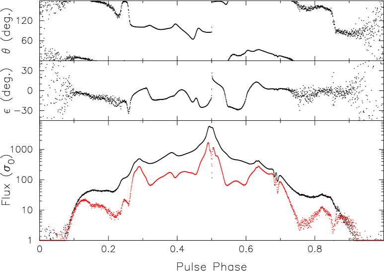
Figure 1.: Mean polarization of PSR J0437$-$4715, plotted using polar coordinates: orientation, $\theta$; ellipticity, $\epsilon$; and polarized intensity, $S=|\mbox{\boldmath$S$}|$ (plotted in red below the total intensity). Flux densities are normalized by $\sigma_{0}$, the r.m.s. of the off-pulse total intensity phase bins. Data were integrated over a 64 MHz band centered at 1341 MHz for approximately 40.6 hours.

2.1. High-Precision Timing

In any high-precision pulsar timing experiment, the confidence limits placed on the derived physical parameters of interest are proportional to the precision with which pulse time-of-arrival (TOA) estimates can be made. Aside from typical observational constraints such as system temperature, instrumental bandwidth, and allocated time, TOA precision also fundamentally depends upon the physical properties of the pulsar, including its flux density, pulse period, and the shape of its mean pulse profile. When fully resolved, sharp features in the mean pulse profile generate additional power in the high frequency components of its Fourier transform. As higher frequencies contribute stronger constraints on the linear phase gradient in the last term of equation (2), sharp profile features translate into greater arrival time precision.

This important property may be exploited in order to significantly improve the precision of arrival time estimates derived from full polarimetric data. As noted by Kramer et al. (1999), the mean profiles of Stokes $Q$, $U$, and $V$ may contain much sharper features than that of Stokes $I$, especially when the pulsar exhibits transitions between orthogonally polarized modes. Although the polarized flux density is lower than the total intensity, these transitions lead to a greater SNR in the high frequency components of the polarized power spectra, as shown in Figure 2.

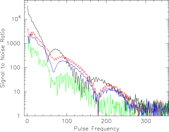
Figure 2.: Power spectra of the standard profile plotted in Figure 1. Stokes $I$, $Q$, $U$, and $V$ are plotted in black, red, green, and blue. Above 40 times the pulse frequency, both Stokes $Q$ and $V$ exhibit a SNR greater than or equal to that of the total intensity.

To demonstrate the potential for improved arrival time precision, TOA estimates spanning over 100 days were derived from the 490 five-minute integrations used to produce the standard plotted in Figure 1. The arrival times derived from the mean total intensity profile have a post-fit residual r.m.s. of 198 ns. By modeling the polarimetric pulse profile as described in Section 1, the resulting arrival times have a post-fit residual r.m.s. of only 146 ns, an improvement in precision of approximately 36%.

2.2. Instrumental Calibration

Based on the assumption that the mean polarimetric pulse profile does not vary significantly with time, the standard profile and modeling method may also be used to determine the polarimetric response of the observatory instrumentation at other epochs. As a demonstration, a single, uncalibrated, five-minute integration of PSR J0437$-$4715 was fitted to the polarimetric standard shown in Figure 1. The model was solved independently in each of the 128 frequency channels, producing the instrumental parameters shown with their formal standard deviations in Figure 3. In each 500 kHz channel, it is possible to estimate the ellipticities and orientations of the feed receptors with an uncertainty of only one degree. This unique model of the instrumental response may be used to calibrate observations of other point sources.

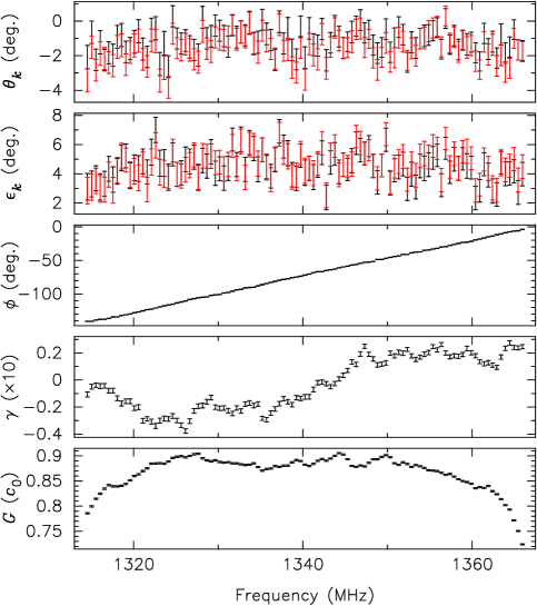
Figure 3.: Best-fit instrumental parameters as a function of observing frequency. A single, uncalibrated, five-minute integration of PSR J0437$-$4715 was fitted to the polarimetric standard. From top to bottom are plotted the orientations, $\theta_{k}$, and ellipticities, $\epsilon_{k}$, of the feed receptors, the differential phase, $\phi$, the differential gain, $\gamma$, and the absolute gain, $G$, specified in units of an intermediate reference voltage that can later be calibrated to produce absolute flux estimates. In the top two panels, black and red correspond to receptors 0 and 1, respectively.

3. Conclusion

When compared with the scalar equation used to model the relationship between total intensity profiles, the matrix equation presented in Section 1 quadruples the number of observational constraints while introducing only six additional free parameters. By completely utilizing all of the information available in mean polarimetric pulse profiles, arrival time estimates may be obtained with greater precision than those derived from the total intensity profile alone. In addition, the modeling method may be used to uniquely determine the polarimetric response of the observatory instrumentation using only a short observation of a well-known source.

Acknowledgments.

The Swinburne University of Technology Pulsar Group provided the CPSR-II observations presented in this poster. The Parkes Observatory is part of the Australia Telescope which is funded by the Commonwealth of Australia for operation as a National Facility managed by CSIRO.

References

Britton, M. C., 2000, ApJ, 532, 1240

Hamaker, J. P., 2000, A&AS, 143, 515

Kramer, M., Doroshenko, O., & Xilouris, K. M., 1999, poster presented at Pulsar Timing, General Relativity and the Internal Structure of Neutron Stars

van Straten, W., 2004, ApJS, 152, in press

Taylor, J. H., 1992, Phil. Trans. R. Soc. Lond. A, 341, 117