M/L, H$\alpha$ Rotation Curves, and HI Measurements for 329 Nearby Cluster and Field Spirals: I. Data

Abstract

A survey of 329 nearby galaxies (redshift z $<$ 0.045) has been conducted to study the distribution of mass and light within spiral galaxies over a range of environments. The 18 observed clusters and groups span a range of richness, density, and X-ray temperature, and are supplemented by a set of 30 isolated field galaxies. Optical spectroscopy taken with the 200-inch Hale Telescope provides separately resolved H$\alpha$ and [NII] major axis rotation curves for the complete set of galaxies, which are analyzed to yield velocity widths and profile shapes, extents and gradients. HI missing line profiles provide an independent velocity width measurement and a measure of HI missing gas mass and distribution. $I$-band images are used to deconvolve profiles into disk and bulge components, to determine global luminosities and ellipticities, and to check morphological classification. These data are combined to form a unified data set ideal for the study of the effects of environment upon galaxy evolution.

1. Introduction

This study concerns the effects of the cluster environment on the distribution of mass and light in spiral galaxies. These data are part of a large survey of nearby clusters (redshift $z\leq 0.045$) designed to study the dependence of mass–to–light distributions upon cluster densities by comparing core galaxies to periphery and low density region members, to evaluate the global properties of rotation curves, and to examine fundamental galaxy properties in varied environments. There are several other large samples of optical rotation curves in the literature at present, including Courteau’s 1992 sample of 350 which focuses primarily upon field galaxies, and Mathewson & Ford’s 1996 sample of 2447 in the southern hemisphere. This data set contains the rotation curves of 329 northern hemisphere cluster and field galaxies, with HI missing observations for most to provide additional, independent constraints upon mass distributions.

The velocity profiles of spiral galaxies were originally believed to fall in a Keplerian decline at large radii, following an inverse $r$ law near the edge of the optical disk where the light (and presumably mass) dropped off. When the first measured rotation curves did not show such a trend they were assumed to probe only the inner region, rather than that predicted to exist at large radii for a pure exponential disk model. As hardware improvements extended the sensitivity and depth of observations, however, more and more of the outer regions of galaxy disks were observed. It became clear that both optical and 21 cm line observations showed velocity profiles which rose in the inner regions but often remained flat at their outer extents, implying the presence of a considerable amount of dark matter within the optical radius (cf. Bosma 1978, review by Faber & Gallagher 1979).

In the early 1980’s Rubin and collaborators began a pioneering study of spiral galaxies to attempt to constrain mass distributions by analyzing optical velocity profiles and light distributions (Rubin, Burstein, Ford, & Thonnard 1985, and references therein). They deduced that velocity profiles correlated well with basic galaxy properties as luminosity (brighter galaxies having larger velocity widths which rose more slowly) and morphological type (earlier type galaxies having larger velocity widths). This initial sample of field galaxies was later extended to include a set of cluster spirals (Burstein, Rubin, Ford, & Whitmore 1986; Rubin, Ford, & Whitmore 1988; Whitmore, Forbes, & Rubin 1988), to evaluate the importance of the cluster environment upon the mass distributions. They found a population of cluster galaxies with rotation curves which appeared to decline at large radii, and argued that these galaxies had deficient halos which had either been stripped through an interaction with the cluster medium (e.g., ram pressure sweeping) or with close neighbors (tidal stripping), or had never been allowed to form. Later studies (Guhathakurta et al. 1988; Forbes & Whitmore 1989; Distefano et al. 1990; Amram et al. 1993; Adami et al. 1999) found conflicting results regarding these trends, and thus part of the motivation for this work has been to re-examine these claims within a larger sample of galaxies.

The strong effect of the cluster environment upon the HI missing gas envelope of spiral galaxies has been well established (cf. Haynes & Giovanelli 1986, Magri et al. 1988, Haynes 1989, Solanes et al. 2001). Galaxies interacting with the hot intracluster medium of moderate to high X-ray luminosity clusters are observed to be strongly HI missing deficient and to have lost HI missing gas preferentially at outer radii (Haynes 1989), and the pattern of HI missing deficiency correlates strongly with clustercentric radius. The stripped galaxies appear to have an undisturbed spiral morphology, though biased towards early types, implying that the mechanisms in play are either too weak to directly affect the stellar material or that the effect can only be recognized on a longer timescale (e.g., decreased young star formation from a depleted HI missing gas reservoir).

This paper is the first of three in a series. The present paper (Paper I) details the observations which were made in the optical and in the radio, and defines the data analysis procedures and the modeling technique used to determine mass-to-light ratios for the galaxies within the sample. The second paper (Vogt et al. 2004a; Paper II) investigates the evidence for galaxies which are currently infalling into the cores of clusters on a first pass, or show evidence of a previous passage through the core, and the role of gas stripping mechanisms in a morphological transformation of the field spiral population into cluster S0s. The third paper (Vogt et al. 2004b; Paper III) explores differences in fundamental galaxy properties (size, mass, and luminosity) as a function of environment, whether spiral disks within rich cluster cores may have coalesced from their halos at an early epoch, and examines the relationship between HI missing gas stripping by the hot intracluster medium and the consequential suppression of young star formation across the disks.

2. Sample Properties

2.1. Distribution of Clusters

We have assembled herein the data from an observational program in moderate resolution optical spectroscopy conducted at the 200-inch Hale Telescope, with parallel 21 cm and $I$-band photometric observations, centered upon a set of 18 nearby clusters and an accompanying field sample. The clusters span a wide range in richness, density, and X-ray temperature in order to explore a wide range of environments, with redshifts between 5000 km s^-1 and 12000 km s^-1. They were selected so that part of the sample was overhead at all hours, to enable observations at all seasons and maximize our use of observing time on the project, with a preference for clusters within the Arecibo Observatory declination range ($-1{{}^{\circ}}<\delta<38^{\circ}$). The initial selection of 16 was made from the northern catalog of rich clusters of galaxies (Abell, Corwin, & Olowin 1989), drawing from the Pisces–Perseus, Hercules, and Coma superclusters. We began with six rich clusters for which many HI missing profiles had been already obtained and X-ray flux data existed (see Magri et al. 1988 study of HI missing deficiency): A262, A426 (Perseus), A1367, A1656 (Coma), A2147, and A2151 (Hercules). We added A2152 as it overlaps with A2147 and A2151, and A2197 and A2199 as the companion clusters cover the extremes of rich (A2199) and poor (A2197) environments. More moderate environments were sampled within clusters A400, A539, and A2063, and A2634 and close neighbor A2666, and the poor clusters A779 (chosen also to fill a gap at $\alpha\sim 10^{h}$) and A2162 (selected but observations barely begun). The sample was then augmented by the Cancer (CGCG0819.6+2209) and NGC507 (CGCG0150.8+3615) groups. The cluster distributions were evaluated after the observations were completed and membership criterion imposed to separate true cluster members from those associated with the cluster in the nearby supercluster envelope and foreground and background field galaxies (see discussion in Paper II). Table 1 lists the cluster positions, redshifts, and parent supercluster structures, and Figure 1 shows their distribution upon the sky. Redshifts are presented in the heliocentric and the CMB reference frames (see Kogut et al. 1993 for relative relations). A number of these clusters were analyzed in the peculiar velocity study of Giovanelli et al. 1997; coordinates and redshifts are consistent between the two presentations.

Table 1Distribution of Clusters

Cluster	R.A. $\;\;(1950)\;\;$ Dec.		Redshifta		$R_{A}^{b}$	Supercluster	References
(1)	(2)	(3)	(4)	(5)	(6)	(7)	(8)
N507	01 20 00.0	+33 04 00	5091	4808	1.74	Pisces-Perseus	1
A262	01 49 50.0	+35 54 40	4918	4664	1.81	Pisces-Perseus	1
A400	02 55 00.0	+05 50 00	7142	6934	1.25	Pisces-Perseus	2
A426	03 16 20.0	+41 20 00	5460	5300	1.63	Pisces-Perseus	3
A539	05 13 54.0	+06 25 00	8730	8732	1.04	$\cdots$	4
Cancer	08 17 30.0	+21 14 00	4705	4939	1.91	$\cdots$	5
A779	09 16 48.0	+33 59 00	6967	7211	1.30	$\cdots$	2
A1367	11 41 54.0	+20 07 00	6408	6735	1.38	Coma	2
A1656	12 57 24.0	+28 15 00	6917	7185	1.29	Coma	6
A2063	15 20 36.0	+08 49 00	10445	10605	0.86	Hercules, southern	2
A2147	16 00 00.0	+16 02 00	10493	10588	0.87	Hercules, canonical	7
A2152	16 03 07.0	+16 35 00	12930	13018	0.72	Hercules, canonical	7
A2151	16 03 00.0	+17 53 00	11005	11093	0.83	Hercules, canonical	7,8
A2162	16 10 30.0	+29 40 00	9600	9659	0.95	Hercules, northern	9
A2197	16 26 30.0	+41 01 00	9138	9162	0.99	Hercules, northern	2,10
A2199	16 26 54.0	+39 38 00	8970	8996	1.00	Hercules, northern	2,10
A2634	23 35 54.9	+26 44 19	9240	8895	0.98	Pisces-Perseus	11
A2666	23 48 24.0	+26 48 24	8118	7776	1.11	Pisces-Perseus	2,11
aHeliocentric and CMB reference frames.
bAbell radius (degrees).
References. — (1) Sakai, Giovanelli, & Wegner (1994), (2) Zabludoff et al.
(1993a), (3) Kent & Sargent (1983), (4) Ostriker et al. (1988), (5) Bothun
et al. (1983), (6) Kent & Gunn (1982), (7) Barmby & Huchra (1997), (8) Bird,
Dickey, & Salpeter (1993), (9) Abell (1958), (10) Dixon, Godwin, & Peach
(1989), (11) Scodeggio et al. (1995).

We began by characterizing the clusters by a set of criteria, including the Abell richness class, the diffuse X-ray gas luminosity and temperature, the velocity dispersion, and the HI missing deficiency of member galaxies. The Abell classification serves as a robust measure of cluster richness, defined by the number of bright galaxies within one $R_{A}$ (1.5 h^-1 Mpc). Rich clusters are also distinguished by the presence of a large, diffuse envelope of hot X-ray gas, of order $10^{42}$ to $10^{45}$ ergs $s^{-1}$ (Beers et al. 1991), with a flux distribution only roughly equivalent in some cases to that of the individual galaxies (the luminous matter). This material can comprise up to 30% of the mass of a cluster (Dell’Antonio, Geller, & Fabricant 1995). It is accreted from the surrounding 10 – 20 Mpc (David 1997), in contrast to the dark matter, which can be accounted for entirely by the stripping of individual galaxy halos.

Dynamically evolved, centrally condensed clusters such as A1656 have high X-ray luminosities and intergalactic gas temperatures and the X-ray flux is distributed smoothly throughout the cluster. In contrast, less evolved rich clusters such as A2634 have lower X-ray luminosities and temperatures and the X-ray intergalactic gas is clumped about individual galaxies, suggesting recent emission or gas stripping by ram pressure (Gunn & Gott 1972) or tidal forces (cf. Toomre & Toomre 1972, and more recently Weinberg 1996). The X-ray gas distribution and temperature serves as an indicator of the overall state of the cluster: the X-ray temperature correlates tightly with the velocity dispersion (i.e. the depth of the potential well), while the X-ray luminosity reflects the density of the intracluster medium.

Figure 1.— The cluster sample shown on an Aitoff equal area projection of the celestial sphere, centered at 12 hours. Heavy lines define the galactic plane and $\pm 20^{\circ}$ about it.

HI missing deficiency, in contrast, is as a specific indicator of the local environment around a particular galaxy. By observing the morphology-density relation (cf. Dressler 1980a), number counts of galaxies, and HI missing deficiency statistics, we gain a measure of the previous interaction history of member galaxies, with both the intergalactic medium and with other galaxies within the potential. We are thus able to characterize the range of our sample, from such highly evolved clusters as A1656 and A426, to the loose groups of Cancer and NGC507, to isolated field galaxies.

2.2. Galaxy Selection

An initial search was made of the Upsala General Catalog (UGC, Nilson 1973) for sources which fell within several $R_{A}$ of the target cluster centers (the total sample is heavily concentrated within one $R_{A}$). Extensive use was made of the source lists contained within Dressler’s catalog (1980) of rich clusters, and the accumulated sources already entered into the 1994 version of the private database of R.G. and M.P.H. known as the AGC, containing a large number of galaxies observed with the Arecibo Observatory 305–meter radio telescope and/or the 300–foot NRAO telescope in Green Bank. A visual examination was then conducted of the POSS prints of the region surrounding each cluster center for additional sources. Galaxies were chosen on the basis of apparent cluster membership (i.e. within several $R_{A}$ of the target cluster centers, note that redshifts were unknown for many sources before the observations began) and spiral appearance and morphology, with no evidence of current interaction with other sources or overlapping field stars to obscure the profiles. Roughly 12% of the selected galaxies are barred systems. The sources were prioritized to have an angular size $\theta\geq 30$″, and an inclination angle $i\geq 30^{\circ}\ (b/a\leq 0.87)$. The clusters were examined from the center outwards, focusing first upon all galaxies within one $R_{A}$ and then adding additional sources further out as observing time permitted. As the optical spectra, and $I$-band images were acquired in parallel over the five year observational period, spectral candidates were at times prioritized within a cluster sample because an image had already been obtained. This was a random effect, however, as the imaging program was designed to lag the spectral and HI missing line profile programs deliberately, so as to be comprised mainly of sources for which we had already obtained a velocity profile. Because of this time lag and the limited amount of observing time available for imaging, several clusters lack substantial imaging and we have no images for A2063.

The sample cannot be said to be strictly limited nor complete in either size nor magnitude, due to the varying inputs into the total set. We conducted a program to evaluate the distances to many of the clusters via the Tully–Fisher (Tully & Fisher 1977) relation in parallel with this project, and thus every effort was made to observe all spiral galaxies which appeared to be members of the target clusters (i.e. neither foreground nor background objects, and without obscuring sources), especially in the inner regions of the clusters. As expected, the fraction of late type spirals decreases within the cluster cores, though such galaxies were prioritized in the selection process; the median type across the complete sample is Sbc.

Figure 2 addresses the issue of sample selection, given the lack of completeness in the selection criteria (note that the sample covers a factor of two in redshift). The data are divided into five narrow redshift bins, and the distinct peaks within each bin are caused by the tight cluster distribution. The distribution of angular size (characterized by R_23.5, the radius at which the disk reaches a surface brightness level of M_I = 23.5 magnitudes per square arcsecond) within each bin can be fit well by a Gaussian curve, given the narrowness of the bins (i.e. the spread in distance is rather small within each bin). We find that a Gaussian of constant width will fit the data across all five bins. The mean of the curve has been shifted to account for the change in apparent size due to distance for the central redshift of each bin, and matches the progression in the data well. The circular velocities are also well fit by a Gaussian, and the constant width and mean suggest that we are sampling galaxies of the same velocity width (mass) at all redshifts. The change in apparent magnitudes mirrors that in apparent size. We fit a Schechter luminosity function to the data within each redshift bin, a technique which works purely because the scatter in distance within each bin is small and so the spread in luminosity is primarily due to intrinsic variation. The point is simply to characterize the change in apparent magnitudes, which are well fit by a luminosity function where M^∗ is set by assuming all galaxies within each bin fall at the central redshift for the bin. The completeness in magnitude can then be observed to fall off at M_I = 13.85, across all redshift bins, below the peak of the luminosity function.

3. Optical Spectra

3.1. Data Acquisition and Reduction

Figure 2.— Exploration of sample selection in the observational plane, showing the sample distribution in redshift, size, circular velocity, and luminosity broken into five redshift bands. A Gaussian function is fit to the size and velocity functions, it is frozen across the redshift bins for velocity and shifted for those in size to account for the change in apparent size on the sky with redshift. A Schechter luminosity function (M^∗=-22.1, $\alpha$=-0.50, assuming the central redshift of each band) is similarly applied to the magnitude histograms and shifted to account for the change in apparent magnitude on the sky with redshift; a dotted line marks where completeness begins to fall off, at M_I = 13.85. The spread of each luminosity histogram is a combination of variations in distance and in intrinsic luminosity, but the first factor is minimized by the narrowness of the redshift bins and the strong peaks due to clustering.

Moderate–resolution long–slit optical spectra were obtained for 329 spiral galaxies with the Hale 200–inch telescope using the Double Spectrograph (Oke & Gunn 1982) at the Cassegrain focus (f/15.7) on 51 nights spread throughout 12 observing runs from April 1990 to June 1994. The red (5200 - 11000Å) camera was used with one of two TI 800$\times$800 chips, with a 1200 l mm^-1 grating (7100Å blaze) yielding a resolution of 0.81 Å pixel^-1 for 15$\mu$ pixels. The camera has a spatial scale of 0″.58 pixel^-1 and the 1″$\times$ 125″slit was used (only one galaxy within the sample extended beyond a slit edge in H$\alpha$). We observed the appropriately redshifted [NII] line pair ($\lambda\lambda$6548, 6584), H$\alpha$ ($\lambda$6563), and the [SII] line pair ($\lambda\lambda$6717, 6731) by obtaining spectra over the wavelength range $6300\leq\lambda\leq 7000$, with a resolution in velocity space of 37 km s^-1 per pixel. Note that at a redshift $z$ = 0.045 H$\alpha$ is redshifted to a wavelength of $\lambda$6858, comfortably within our upper limit.

The spectrograph was rotated to align the slit along the major axis of the source with an accuracy greater than that of the position angle measurement ($\pm 2^{\circ}$, measured from sample $I$-band images or Palomar Optical Sky Survey prints). The seeing conditions ranged from 0″.8 to 2^′′ and were usually under 1″.5. Because of this, neighboring 0″.58 pixels are not independent. Sources were observed on average at less than 1.2 airmasses, and never at more than 1.5 airmasses. Exposures ranged from 2400 to 3000 seconds in length. As the project progressed, integration times were lowered slightly from the nominal value of 3000 seconds for all but the most distant clusters in order to observe more sources per night, as the S/N ratios were quite high in the observed emission lines.

The data were reduced using standard Image Reduction and Analysis (IRAF) routines and custom software. The CCD was aligned so that the spectra were dispersed along the columns, and the spatial axis ran along the rows. Flat fields were created from dome flats taken with high intensity white light lamps, and standard stars were placed in a series of five positions across the slit twice each night to correct for S–curve distortion along the chip (0.1 to 0.2 pixels). Spectra were wavelength calibrated directly from the strong night sky emission lines as they spanned the wavelength range observed quite well, and to avoid the problems of variable spectrograph flexure which appeared in the lamp spectra taken directly before and after each exposure.

A region was marked on each spectrum beyond the extent of the disk emission (for all but the most spatially extended galaxies), and used to calculate an average background level across the chip. This background was then subtracted, to remove the strong night sky line emission which fell near or on top of the galaxy emission lines. A running (boxcar) average was applied across the chip in a box three columns wide, to smooth the data slightly. A Gaussian fitting routine was then applied to each column of data in the zone about the H$\alpha$ line, fit in either emission or in absorption, and then the stronger [NII] line ($\lambda$ 6584) to trace the velocity profile across the optical disk. The [SII] line pair ($\lambda\lambda$6717, 6731) had been redshifted into a wavelength range which is heavily contaminated by night sky lines for most of the galaxies in this sample, and thus the lines could not be well fit. Criteria were set for the quality of the fit at every column: an amplitude requirement (5$\sigma$), a width requirement (3$\sigma$), a limit on the line width (1 - 10Å), and a limit on the distance that the line centerpoint could shift between two columns (5 pixels). This fitting process was iterated until the fit of the lines was found to be adequate. The final fits are good to within 5 km s^-1.

3.2. Comparison with Literature Data

The first significant sample of optical rotation curves was acquired by Vera Rubin and her collaborators in the early 1980’s, taken on photographic plates with the KPNO and CTIO 160–inch telescopes. We have re-observed six galaxies in the Rubin sample; the spectra and derived H$\alpha$ rotation curves are found to be in good agreement, as one would expect given the similarity of observational techniques. In Figure 3A and B we compare the data for two common galaxies, UGC11810 (NGC1401) and UGC5250 (NGC2998). The overall structure is the same in both set of spectra, though as the Rubin data has been smoothed significantly it shows less of the small scale variations seen in our data. Their data appear to extend slightly further out along the galaxy disks, though of course such measurements are a strong function of the fitting constraints applied to extracting rotation curves, but the additional data points does not show additional structure in the rotation curves.

The extensive data set of Mathewson & Ford (1996) is certainly worthy of note; however, due to its southern declination we do not overlap. More recently, Courteau (1992, 1997) has presented CCD longslit spectroscopy from the Shane 120–inch of H$\alpha$ and [NII] lines for 304 spiral galaxies. We have observed 23 galaxies in common; a comparison plot of the full set can be found within Courteau 1997, and is thus not included here. Courteau’s data were obtained primarily to determine a full velocity width for each galaxy rather than to examine the structure of the entire rotation curve, and so are not as deep. Our observations have a higher S/N ratio due to longer exposures times (50 minutes versus 25 – 30 minutes) and a larger aperture. Taking this into account, we find good agreement between the two data sets. The radial extents of the profiles are similar, and much (though not all) of the small scale structure is confirmed in each set.

Figure 3.— Rotation curves from our sample and from the literature for overlapping sources, plotted on top of each other for comparison. The H$\alpha$ profiles are uncorrected for inclination and in the rest frame of the galaxy; small circles represent our data, squares (A and B) the data of Rubin et al. (1982, 1980), and triangles (C and D) the Fabry–Pérot data of Amram et al. (1994). As Amram et al. (1994) collapse their two–dimensional velocity maps to a radial profile, we have reflected this radial data about the centerpoint to simulate the two sides of the galaxy observed in a longslit. The observations agree well, though the Fabry-Pérot extends further out in the galaxy due to increased S/N, and shows less small scale structure due to azimuthal smoothing.

Longslit spectroscopy observations are handicapped by the fact that they sample only along the (major) axis of a galaxy, and thus are extremely sensitive to the (1) detection, and (2) localized non–circular motions of individual HII missing regions or spiral arm structure along this axis. An excellent alternative technique is to acquire full two dimensional velocity maps via interferometry. Fabry–Pérot data sets typically penetrate further and with greater S/N in the outer regions of galaxies, and full velocity maps allow a more sophisticated deprojection of velocities into the edge–on plane by fitting a series of disks of varying inclination as a function of radii, and modeling for warps and substructure as a function of azimuth. The costs, however, in both observing and analysis time, can be high, and to date have limited the number of galaxies analyzed via this technique. Amram et al. (1992, 1994) used the 140–inch CFH telescope to obtain two–dimensional H$\alpha$ maps for 36 galaxies within nearby clusters (13 of which fall within our sample), and the GHASP project (Garrido et al. 2002, 2003) has recently published similar data for 38 galaxies out of an observed sample of over 160 field spirals and irregulars. Figure 3C and D overlay the optical rotation curves from our data and from Amram et al. for UGC1437 (NGC753) and UGC1238 (NGC668). As expected the Fabry–Pérot data extends roughly 30% further out in the outer regions of the galaxy, and, being smoothed azimuthally, shows less small scale, localized variations. The curves agree well on global structure, however, and within the inner arcminute radius sampled within our data the terminal behavior of the velocity profile is well established.

We have compared the common galaxies within our sample and several from the literature to establish the equivalence of techniques of observation and analysis between various practitioners of longslit spectroscopy. Though not shown here explicitly, our data acquisition and reduction techniques are also in good agreement with the published work of Dale et al. (1997, 1998, 1999), which shares many common elements. More extensive comparisons could be made with a broader range of data sets (e.g., Corradi & Capaccioli 1991), but we have shown sufficient consistency in form for our purpose. While Fabry–Pérot observations give additional information regarding the detailed velocity structure of galaxy disks, the global properties obtained via longslit work are in agreement with those derived from these measurements.

3.3. Data Characterization and Analysis

We begin by visually characterizing the optical spectra; Figure 4 shows a subset of four galaxies ranging from type Sa through Sc. These moderate resolution data show a clear separation between the H$\alpha$ and [NII] lines, and the velocity profiles of the two species exhibit similar global behavior and structure. The H$\alpha$ flux is generally stronger than that of the [NII] at a given position, and tends to extend slightly further to large radii. Both are sensitive to the positioning of individual HII missing regions along the slit and can become patchy when traced along a late type disk with strong spiral arms, where the regions between the arms have been swept clean of gas. The [NII] lines tend to be better resolved in the nuclear region. The H$\alpha$ line, in contrast, can broaden appreciably and may be derived from clumps of gas traveling at noncircular (i.e. random) velocities. The presence of a bar often creates a plateau, or a local maximum, in velocity at the end of the bar, as shown for UGC1013 in Figure 5F. The emission extends out to a mean value of 3.7R_d. It can be traced past 2.2R_d, the point of maximum velocity for a pure exponential disk (Freeman 1970), for all but the lowest quality data and a number of galaxies with strong bars, where R_d has been measured to be quite large ($>10$ kpc).

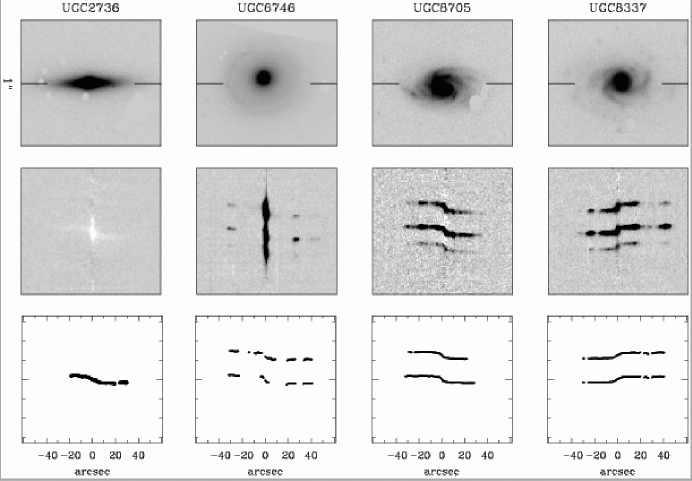
Figure 4.— We illustrate the characteristics of the sample with four galaxies; scales are identical and spatial axes aligned for each set of three plots. The upper image shows the $I$-band data for each galaxy, with the width of the longslit represented as a black line. The lower image is of the optical spectrum centered about the H$\alpha$ line and companion [NII] lines, with the bulk of the continuum removed to reveal the shape of the rotation curve in the inner regions. The lower plot shows the rotation curve fit to H$\alpha$ and to the stronger of the two [NII] profiles. UGC2736 is typed as an Sab, and shown because the H$\alpha$ line is found purely in absorption, representative of an older stellar population; less than 10% of the sample shows no H$\alpha$ emission. UGC6746 one of the few Sa galaxies in the sample,, UGC8705 an Sb galaxy, and UGC8337 an Sc galaxy; these particular galaxies were chosen because their face-on orientation makes the spiral structure easier to observe in the images, but are otherwise representative.

The first galaxy in Figure 4, UGC2736, is shown as it exhibits no [NII], and the H$\alpha$ line is found purely in absorption. We note that at high inclination angles the morphological distinction between an early-type spiral galaxy and an S0 becomes more difficult to discern, because the spectra are composed primarily of light from the older stellar populations of the disk (see discussion in Paper II). There are less than 30 such spectra in the sample. The next three galaxies were selected because they were less inclined than average, to allow easy examination of the spiral structure along the longslit, but are otherwise representative of the sample (though recall that the median type is Sbc). The strength of the flux along the disk is a clear function of the spiral arm structure, and indeed much of the disk of the Sa galaxy is extremely faint.

Rotation curves were created for the entire data set by combining the H$\alpha$ and [NII] data together to create unified velocity profiles. The rotation curve of a normal spiral galaxy can be characterized by three regions. There is a steeply rising inner region, a transition zone (often called the elbow point) where the rotation curve turns over, and then an outer region which is roughly linear (like the inner region) and often flat. We find the overall shape of the rotation curve to be more a function of luminosity than of morphological type, as reported by Rubin, Ford, & Whitmore (1988), indicating that optical morphology is not a strong measure of the underlying gravitational potential. The terminal velocities correlate strongly with luminosity, as expected from the Tully–Fisher relation, and the higher luminosity galaxies also have rotation curves which rise more quickly to their terminal value than the lower luminosity sources (characterized by gentler curves with wider transition zones).

The spectra were binned according to quality and to rotation curve shape. The 278 quality (1) rotation curves are well defined (traced) and well sampled, the 45 quality (2) curves are of fair quality; the curve is untraceable at certain points along the disk (due either too weak H$\alpha$ flux or to the inference of [OH] emission lines), and the six quality (3) curves do not adequately map the velocity profile of the galaxy (the H$\alpha$ flux is too weak or the galaxy is too face–on). The shape scale is sensitive to the slope of the rotation curve, particularly in the outer region, and defined as follows: the 120 (1) curves are flat in their outer regions, and evenly terminated, the 128 (2) curves are almost flat and yet slightly rising in their outer regions, the 57 (3) curves terminate with a rising profile, and the 12 (4) curves exhibit a pattern of solid body rotation, being lines of one continuous slope with no turnover, or elbow, point or inflection recorded in the emission line profile. Examples of all four types are shown in Figure 5. Twelve of the rotation curves fit none of these shape categories, five being too face–on for the velocity profile to be well mapped, two having disturbed curves with strong distortion from a smooth shape, and five (all of quality 2 or 3) either too poor in quality or too sparse in coverage of the disk to be well fit.

Figure 5.— Sample rotation curves illustrating the range of shapes within the data: (A) UGC8460, with a flat $Q_{sh}$= 1, (B) UGC1459, with a slightly rising $Q_{sh}$= 2, (C) UGC1248 with a rising $Q_{sh}$= 3, and (D)AGC211029 with a solid body curve ($Q_{sh}$= 4). For (E) AGC210727/CGCG097-125 the two sides of the rotation curve are traced to very different extents, and for (F) UGC1013 (barred) the velocity of the inner regions is higher than the terminal velocity profile. The H$\alpha$ points are filled circles and the [NII] data are open circles; error bars are plotted only when greater than 10 km s^-1.

Each calibrated spectrum was visually inspected and (rarely) single points were removed from the fitted rotation curve if they were believed to be contaminated by night sky lines or a cosmic ray residual. A global centerpoint was then measured for each galaxy, and the data were transformed from wavelength to restframe velocity space. This enabled the rotation curves to be folded into a radial profile, so that they could be compared to the luminosity profiles for agreement of structure and used to create mass models. Velocity widths were measured to check for variations in the terminal velocities relative to those measured from the 21 cm line, and to calculate deviations from the Tully–Fisher relation. Slopes were fit to the inner and outer portions of each rotation curve and functional fits were also applied to the form of the rotation curve, to permit quantitative comparisons between galaxies.

The centerpoint of each spectrum in wavelength and on the sky was estimated in two ways. First, the wavelengths were binned into a histogram, and cuts were made into each side at the 10% level to remove scattered and outlying points. The two endpoints of the trimmed histogram were averaged to determine the cardinal central wavelength of the galaxy. The spatial and wavelength centerpoint of the rotation curve was then defined to lie at the location of the nearest data point. If the galaxy could not be traced through the nuclear continuum in either H$\alpha$ or [NII] (see Figure 5E), the spatial centerpoint was allowed to “float” to a column with no data, and the cardinal wavelength value was used as the wavelength centerpoint. Second, the point closest to the center–of–light (COL) determined from fitting the peak of the galaxy continuum was chosen to be the spatial centerpoint, and the wavelength of that point to be the central wavelength of the system.

Default central values are those determined from the endpoints of the histogram of wavelengths. For 40 galaxies, however, the COL value is more representative. The spatial centerpoint for these galaxies differs by more than two arcseconds when measured via the two techniques. In the case of such disagreement, the COL values were taken to be more accurate, and were used. We also folded each rotation curve at the centerpoint to create two radial profiles which were plotted on top of each other, and verified that the curvature of the inner region of the rotation curve matched from profile to profile. In these cases, using the COL coordinates for centering decreased the deviations between the two radial profiles.

The central wavelength was then converted to a restframe velocity, as discussed in Vogt 1995. The central redshift $z_{c}$ was taken to be the redshift of the galaxy, corrected first to a heliocentric reference frame and then to the reference frame of the Local Group according to the formulation

$$cz_{LG}=cz_{\odot}+300\,\sin l\,\cos b$$ (1)

where $l$ and $b$ are the galactic longitude and latitude.

3.3.1 Velocity Widths

Velocity widths were measured in several ways from the optical spectra. First, the velocity data were binned into a histogram, as above, and cuts were made of a certain percentage into each side (the default being 10%). Though this process bears an apparent resemblance to the fitting of a 21 cm profile by making cuts in frequency space, it is only superficially analogous. The rotation curve is a spatially sampled curve, with no flux weighting given to the data points. A clipping algorithm is used to eliminate scattered outlying points which deviate from the curve and high velocity points in the innermost regions from bars (see Figure 5E); a curve which has leveled off in the outer regions has a fairly constant velocity near the spatial endpoints. The velocity width of the galaxy was then taken to be the difference between the velocity at each endpoint of the trimmed histogram. A second technique is designed for galaxies which are asymmetric or have unbalanced arms (e.g., strong HII missing regions have been traced much further out into the disk along one side than the other, and so a more extended velocity profile can be derived, see Figure 5E). The velocity data were again binned, and cuts were made on each end. Two velocity half widths were defined by comparing the velocity of each endpoint with that of the center of the galaxy as defined by the COL. The full velocity width was then set to be twice that of the half width measured further out along the disk. In the case of AGC210727/CGCG097-125, for example, the velocity half width measured on the left side of the galaxy is 30 km s^-1 higher than that measured on the right side, because it is based upon an inner peak in the velocity profile. We have thus chosen to double the half width measured from the right side of the galaxy in determining the full width of the system.

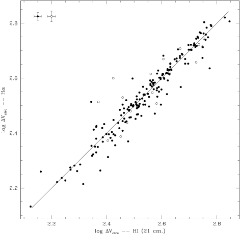
Figure 6.— Velocity widths derived from both H$\alpha$ optical spectra and 21 cm line profiles, showing a clear linear relationship. Solid circles represent high quality data, and open circles data for which one or both of the velocity widths are derived from poor quality spectra. The two points in the upper-left corner display representative median error bars for high and low quality data. We find $\Delta V_{circ}$ (H$\alpha$) = (1.03 $\pm$ 0.02) $\times$ $\Delta V_{circ}$ (HI) $-$ (0.013 $\pm$ 0.008).

A final velocity and velocity width were selected for each galaxy by examining all of the data, taking into account the structure of the velocity profile. The 12 curves of shape class 4, exhibiting solid body rotation, proved to be better fit by measuring the endpoints of the total velocity histogram as the velocity profile continued to rise appreciably in the outermost regions. For these galaxies the data were trimmed only of outlying deviant points, (e.g., isolated points at the end of the rotation curve with an error bar two to three times higher than the norm lying more than 10 km s^-1 above or below the rest of the curve), and the histogram endpoints were then used to calculate the velocity width. For the other rotation curve shapes the standard trimmed histogram technique functioned well. It removed outlying points and a certain amount of scatter, and minimized the effect of large velocities in the inner regions upon the total rotation curve. The key to any technique is a consistent and uniform application, however, which has been achieved with the current method.

It is interesting to compare velocity widths taken from optical spectra with those determined from 21 cm line profiles (cf. Courteau’s 1997 detailed discussion of various techniques, and weighted comparisons, for extracting widths from several samples in the literature). We initially applied our shape coding to the rotation curves within the subsample of Mathewson et al. (1992) for which both optical spectra and 21 cm line profiles had been processed (165 galaxies). A comparison was made of the optical and radio velocity widths, and a shape dependent correction factor applied to the optical spectra on this basis for the well sampled types 1 through 3 (the number of shape 4 curves is too small for a statistically meaningful correction). The correction is not very large, and as expected is largest for the rotation curves which are rising in their outer regions: the optical velocity width is reduced by 3 km s^-1 for $Q_{sh}$ = 1, increased by 6 km s^-1 for $Q_{sh}$ = 2, and increased by 16 km s^-1 for $Q_{sh}$ = 3. Figure 6 compares velocity widths measured via the two techniques for the current sample, after this correction has been applied. There is a good linear relation over the full regime of interest, given the error budget in both width estimates (see discussion in Giovanelli et al. 1997). An average of y-on-x and x-on-y weighted fits yields the relation (log $\Delta V_{circ}$ (H$\alpha$) - 2.2) = (1.03 $\pm$ 0.02) $\times$ (log $\Delta V_{circ}$ (HI) - 2.2) $-$ (0.013 $\pm$ 0.008). The scatter in the width difference relation is 31 km s^-1, and remains fairly constant across the range of $\Delta V_{circ}$ (between 2.2 and 2.8), comparable to previous results for comparable samples of spiral galaxies (Courteau 1997).

One goal of our program is to explore changes in the fundamental parameters (mass, size, luminosity) of galaxies as a function of environment. We thus need a robust measurement of the velocity width (mass) that is not affected by HI missing gas stripping (which can penetrate well into the central regions of the disk), nor by truncation of star formation (and dependent H$\alpha$ emission) in the outer regions of the disk. We have thus also opted to measure the velocity widths at a distance of two R_d along the disks. The rotation curves were again folded about their centerpoints, and both the H$\alpha$ and [NII] data inspected. These data were then interpolated to derive a representative velocity width at two R_d, after the disk scale lengths had been corrected for the effects of galaxy inclination and for seeing conditions.

For 16 galaxies, the H$\alpha$ flux is in absorption rather than in emission, and the [NII] lines are too weak to be traced. For these galaxies a small correction was made to compensate for asymmetric drift, as the raw velocities were measured from the stellar component. Following the fitting technique laid out in Neistein, Maoz, Rix, & Tonry (1999), we fit the velocity width and the dispersion of the H$\alpha$ line at two R_d, and derive a corrected velocity,

$$V_{cor}^{2}=V^{2}(r)+\sigma^{2}(r)\,\left(2\frac{r}{R_{d}}-1\right)$$ (2)

where $r=2$ R_d (see also discussion in Paper III). For a single galaxy, UGC8069, the velocity could also be measured from the [NII] flux; the values agree to within 10 km s^-1.

3.3.2 Rotation Curve Slopes

Rotation curves can be defined to first order by a steeply rising linear inner region, a short transition zone, and then a linear outer region which levels off to a fairly constant level. Shape differences arise from the relative sizes of the regions, and when the outer region of a curve is truncated or does not level off. Each galaxy profile was first folded about its centerpoint by taking the absolute value of positions and velocities relative to that point. Five points were marked on each rotation curve defining the turnover point and a beginning and ending of an inner and an outer region, each of approximately linear behavior (see Figure 7). A least–squares fit was made to each of the two regions, and these slopes were normalized by the velocity half width, V(R_f), of the galaxy and the radius of the turnover point, R_el. This had the advantage of characterizing the curves with parameters derived solely from the shape of the potential, rather than utilizing an optical radius and adding in the effects of the light distribution. The turnover point is less strictly defined than an isophotal radius, though, particularly for barred galaxies with additional substructure in the inner velocity profile. We define the slopes as

$$S_{in}~{}=~{}\frac{\Delta V_{in}/V(R_{f})}{\Delta R_{in}/R_{el}}~{}~{}~{}\longrightarrow~{}~{}~{}\frac{V(R_{el})}{V(R_{f})}$$ (3)

and

$$S_{out}~{}=~{}\frac{\Delta V_{out}/V(R_{f})}{\Delta R_{out}/R_{el}}~{}~{}~{}\longrightarrow~{}~{}~{}\frac{V(R_{f})-V(R_{el})}{V(R_{f})}~{}\times~{}\frac{R_{el}}{R_{f}-R_{el}}$$ (4)

and note their asymptotic forms for the simple case of two linear regions with a narrow turnover zone (the inner slope reduces to the fractional rise of the rotation curve within the turnover point). In Figure 7 we overlay the slope measurements on sample rotation curves for all shape codes. We observe that the inner and outer regions can be well defined and measured for all of the galaxies, but that for the $Q_{sh}$ = 4 galaxy the turnover point is difficult to constrain. For the pictured two galaxies with inner peaks in the velocity profiles, the inner slope is weighted heavily by that substructure.

Figure 7.— Sample rotation curves of each shape class, overlaid with measured slopes (same galaxies as in Figure 5). Rotation curves have been folded about the centerpoints; H$\alpha$ circles are filled (approaching) and open (receding) to mark each side of the galaxy, and no error bars are plotted. The slopes can be well quantified for galaxies $A$ – $D$, ($Q_{sh}$= 1 – 4), but for those with inner peaks in the velocity profile the inner slope is heavily influenced by the peak behavior (often caused by a bar, as in $F$). Rectangular hatched boxes mark the zones 0 – 15% R_23.5 and 40 – 80% R_23.5, over which the percentage rise of the curve is also measured.

One can also normalize the ranges over which gradients are measured by isophotal radii. $B$-band images, which have been used for this purpose in previous studies (cf. Whitmore, Forbes, & Rubin 1988, hereafter WFR; Amram et al. 1993 & 1996), are strongly influenced by current star formation; we have opted for $I$-band images to be more sensitive to the older, underlying disk population. The cardinal $B$-band R₂₅, the isophotal limit of 25 magnitudes per square arcminute, lies roughly an order of magnitude above background levels. We compare R₂₅ (taken from the RC3 for the 181 galaxies in common with our sample) to $I$-band isophotal radii and find a comparable limit at 23.5 magnitudes per square arcminute, R_23.5 with a median offset of 0″.2 between the two radii (Vogt 1995). We then use R_23.5 to normalize the ranges over which we fit velocity gradients to the rotation curves, for comparison with the literature. It was necessary to determine a rotational velocity for a arbitrary points along each rotation curve. Each rotation curve was folded about its centerpoint, and the H$\alpha$ and [NII] points from both sides of the disk were binned together in a weighted average to produce a non-degenerate radial curve. These data were then smoothed with a low–pass FFT filter, and velocities were calculated at specific points along the curve by using an interpolating routine. Inner and outer slopes of the rotation curves, which we shall label as gradients to distinguish them from slopes as defined above, were then defined to be the percentage rise of a synthetic, smooth rotation curve fit to the data, in the ranges $0-0.15$ R_23.5 and $0.4-0.8$ R_23.5.

Figure 7 shows these fitting regions for a set of rotation curves of various shapes. As observed by WFR, galaxies which are intrinsically brighter and/or of earlier type tend to rise more quickly to their maximum velocity, with a short transition zone, and level off to a constant velocity. The 0.15 R_23.5 point targets the inner region for most of the galaxies, but (like the inner slope measurement described above) is sensitive to inner peaks of the velocity profile. The region over which the outer gradient is measured can frequently extend beyond the terminal point of the rotation curve, and thus when examining the outer gradients the sample must be limited to those galaxies for which R_f $\geq$ 0.8 R_23.5 (roughly 50%). For barred galaxies such as UGC1013 (F), the outer gradient range may extend far beyond the extent of the rotation curve.

We can compare the distribution of $I$ based gradients within our sample with the trends seen within previous data in $B$-band to evaluate global trends, as long as we do not assume a one–to–one correspondence between R₂₅ and R_23.5 for individual sources. There are no systematic offsets or trends between WFR, Amram et al. and ourselves when common galaxies are compared; the outer gradients agree to within the observational errors. A primary finding of WFR, that galaxies with falling rotation curves are found preferentially in cluster cores, has not been reproduced. Studies of optical and HI missing velocity profiles for galaxies in the Virgo cluster (Guhathakurta et al. 1988; Distefano et al. 1990; Sperandio et al. 1995), have not confirmed the trend, and 2D Fabry–Pérot observations (Amram et al. 1993, Amram et al. 1996) of several galaxies within the WFR sample did not find the same velocity gradients. The ranges over which each measurement of the velocity gradients was made were not always the same, and as Amram notes, the inclusion or exclusion of single data points along a moderate resolution rotation curve can have a significant effect upon the measured gradient when there are few points.

Figure 8.— The percentage rise in the H$\alpha$ rotation curves between 0.40 and 0.80 R_23.5 versus clustercentric radius. The observed trend (solid lines) is extremely weak, whether fit to all radii or within 750 h^-1 Mpc, and we do not reproduce the stronger trends observed in smaller samples previously (dashed lines). The inset histogram shows the distribution of galaxies within the sample as a function of clustercentric radius, with the fraction for which the rotation curve extends to 0.80 R_23.5 highlighted.

Figure 8 shows a plot of outer gradient as a function of cluster radius, for 75 galaxies within 10 h^-1 Mpc of a cluster (foreground and background galaxies have been suppressed). The observed trend is exceedingly weak, whether fit to galaxy gradients at all radii (OG = (2.9 $\pm$ 2.8) $\times$ log R + (3.7 $\pm$ 0.4), correlation coefficient $r$ = 0.24), or to those within 750 h^-1 Mpc from a cluster core (OG = (1.5 $\pm$ 8.8) $\times$ log R + (3.9 $\pm$ 4.9), $r$ = 0.02), where one would expect environmental effects to dominate. In contrast, fits to samples of $\sim$20 galaxies have produced OG = 43.2 $\times$ log R + 23.3 (WFR), and the far weaker trend of OG = 12.6 $\times$ log R + 0.5 (Amram). Fits to our data produce an even shallower slope than that found by Amram, and are fully consistent (within 1 $\sigma$) with no correlation. A re-analysis (Adami et al. 1999) of the data of Amram found the observed trend to be stronger in late type spirals and not significant in early types; we do not see the correlation in either type group.

Rubin et al. argued that their evidence for declining rotation curves within clusters implied that the affected sources had deficient halos, which had either been stripped through an interaction with the cluster medium (e.g., tidal stripping, ram pressure sweeping) or with close neighbors (e.g., harassment, mergers) or had never been allowed to form. This sample shows no evidence for a strong correlation between outer gradient and clustercentric radius, and thus provides no support for strong environmental variations within dark matter distributions of cluster spirals relative to the field based on these indicators. We note that for all studies, the analysis has been restricted to those galaxies for which H$\alpha$ flux extends to a minimum of 0.80 R_23.5; the accompanying histogram in Figure 8 shows that this removes a significant fraction of observed galaxies at all radii. The fraction rises to 60% between 300 h^-1 kpc and 3 h^-1 Mpc but is lower both in peripheral regions and in cluster cores, suggesting that underlying sample bias (e.g., what portion of the total galaxy population falls within the complete sample) is also relevant. This factor could alter the observed effect (e.g., stripped galaxies have less extended H$\alpha$ flux; see discussion in Paper II).

3.3.3 Rotation Curve Fits

Analytic functional fits were applied to the data to enable the fitting of mass–to–light ratios. A large scale fit, demonstrated in Figure 9, was made to each rotation curve, of the form

$$V(r)=a_{1}(1-e^{a_{2}r})(1+a_{3}r+a_{4}r^{2})$$ (5)

where the global form of the profile was determined by $a_{1}$ and $a_{2}$ (i.e. a two parameter fit), and $a_{3}$ and $a_{4}$ mapped the curvature in the outer regions and could be set to zero to reduce the final term from quadrature to linear or constant order. The coefficients interact to create a model curve such that $a_{1}$ scales with the maximum width of the curve, $a_{2}$ softens the curvature of the turnover point and shifts it along the spatial axis, and $a_{3}$ and $a_{4}$ control secondary curvature displayed primarily in the outer regions of the curve. Note that $a_{1}$ is not equivalent to the asymptotic velocity of the profile, but can assume values much larger when a rotation curve with a very soft turnover region is fit. The fit can be modeled on the total spectral data or on the H$\alpha$ data alone; typically the [NII] data were included unless they were of poor quality. The purpose of the analytic fit was to provide a quantitative smoothed form of the rotation curve, so that a representative velocity could be calculated for an arbitrary point along the disk. The exponential form was chosen purely for convenience, not because of a particular embodiment of physical variables, and is but one of a number of possible and appropriate fitting models (cf. the Universal Rotation Curve model of Persic & Salucci 1990, model fitting by Rix et al. 1997, the arctangent function of Courteau 1997, Polyex fit of Giovanelli & Haynes 2002).

Figure 9.— Sample rotation curves of each shape class, overlaid with measured fits (same galaxies as in Figure 5). Rotation curves have been folded about the centerpoints; H$\alpha$ circles and [NII] triangles are filled (approaching) and open (receding) to mark each side of the galaxy, and no error bars are plotted. Galaxies of $Q_{sh}$ = 1 – 4 can be well traced by the simple exponential form for the fit, as shown in $A$ – $D$. Curves with a strong inner peak in the velocity profile require the higher order terms, and are more difficult to trace, as illustrated in $E$ – $F$.

3.3.4 Mass Distributions

The mass distribution of a galaxy can be determined solely from the observed rotation curve by way of several simplifying assumptions (cf. Rubin et al. 1985). By assuming that the observed rotation curves are a valid measurement of circular, co-planar motion within the gravitation potential of the galaxy, and that the mass distribution is spherically symmetric, the integral mass distribution can be defined as

$$M(r)=2.3265\times 10^{5}\;V^{2}(r)\;r\;\;M_{\odot}$$ (6)

where $V$ is measured in km s^-1 and $r$ in kpc. Mass curves can then be defined by taking the logarithm of the galaxy mass and radius, subtracting off the offsets $M_{m}$ and $R_{m}$ from the centers of the curves, and creating a set of curves centered about a single point. Burstein & Rubin (1985, see also Burstein et al. 1986) determined for the sample of Rubin et al. such integral mass curves, as a means of evaluating the total mass as a function of radius. They defined three mass types of systematically increasing curvature. The type I mass curve was originally determined by fitting a sample of 21 field Sc galaxies (Burstein et al. 1982), type II was created as an intermediate form between I and III, and the mass curve for type III is that of a massless disk in co-planar rotation with an isothermal sphere (Burstein & Rubin 1985). These three curves map out a fairly narrow range in the two-dimensional $\left<M(v,r),r\right>$ space; it is interesting to note that almost all spiral galaxies examined to date can be fit fairly well with one of these three curves. Note that as the derived mass depends linearly on radius, a rotation curve which is flat at large radius (i.e. displays constant velocity) will be transformed into a mass curve of linear slope in the outer regions. Mass types were assigned for our sample of 329 galaxies by evaluating the H$\alpha$ rotation curves, the [NII] rotation curves in the cases where the H$\alpha$ data was deficient (due to weak tracing or strong absorption), and model fits to the combined data sets. It was found that there existed a small number of galaxies with less curvature than the mass types I through III, and thus a type 0 was created to hold these nine outliers.

4. HI Observations

Thus paper incorporates HI missing data obtained in the course of this and other projects, available in a digital archive. The bulk of the HI missing observations were made with the Arecibo Observatory 305–meter telescope. The three northernmost clusters A426, A2197, and A2199 in the range $(39^{\circ}\leq\delta\leq 41^{\circ})$ have been observed with the former 300–foot NRAO telescope in Green Bank (Freudling, Haynes, & Giovanelli 1988, 1992; Haynes, Magri & Giovanelli 1988). All galaxies targeted for optical rotation curve studies were included in a dedicated 21 cm line program (Haynes et al. 1997); the techniques of data acquisition and analysis are discussed in detail therein and in Giovanelli et al. 1997. A total of 304 of the 329 galaxies were successfully observed, and 260 were detected. The data were binned according to quality, Q_HI. The 245 quality (1) line profiles are well defined and well sampled, the 13 (2) profiles are marginal but still usable for measurements of velocity width, the two (3) spectra have detected fluxes but valid velocity widths cannot be measured, the 44 (4) spectra are nondetections, and we do not presently have good data on the 25 (0) objects (eight of which were observed but for which the data are unusable due to strong interference or known source confusion).

The 21 cm line fluxes were calculated by correcting the observed flux, measured at a level of 50% of the profile horns, for the effects of random pointing errors, source extent, and internal HI missing absorption (Haynes & Giovanelli 1984; Giovanelli et al. 1995). The HI missing gas masses were calculated by placing galaxy cluster members at the true cluster distance, and non-members at individually derived redshift-dependent distances (see Paper II for discussion of cluster membership criteria). HI missing deficiency is determined by comparing the observed HI missing gas mass with the expected HI missing gas mass (Solanes et al. 1996). The expected HI missing gas mass is calculated from galaxy morphological type and linear diameter, using blue major axis diameters taken from the UGC (or converted to UGC form from RC3 data) when available and otherwise estimated from the Palomar Optical Sky Survey (POSS) prints. Morphological typing was done through visual examination of plate reproductions of the POSS-I prints at Cornell University, which have a more extended dynamic range than do the standard POSS prints, comparison with the UGC published type codes for UGC galaxies, and (infrequently) updated upon detailed examination of our own $I$-band data. The accuracy is of order $\pm\frac{1}{2}$ Hubble type overall.

For cases where no 21 cm line flux was detected, an upper limit has been placed upon the source strength based on the rms noise per frequency channel, $\sigma$, and the full velocity width, $\Delta V$, based on the optical rotation curve of the galaxy. We assume a simple linear flux model at a level of 1.5$\sigma$ across the full velocity profile, such that

$$S(max)=1.5\;\sigma\;\times\;\Delta V\;\;\mbox{Jy km s}^{-1}.$$ (7)

The application of this HI missing deficiency estimation is problematic, given that the calibrating field galaxies in the Solanes et al. sample have a larger average angular diameter than those within this sample. This incompleteness will lead to an underestimation of the HI missing deficiency, particularly for the smallest (diameter $D_{L}\leq 60^{\prime\prime}$) galaxies within the sample (see Giovanelli, Chincarini, & Haynes 1981). Figure 10, however, confirms that there is no strong trend in HI missing deficiency with angular diameter.

Figure 10.— Plot of HI deficiency versus blue light angular diameters; there is no strong correlation. Nondetections (observational lower limits on HI deficiency) are drawn as open circles; they have been redistributed using survival analysis.

A survival analysis was conducted on the distribution of nondetections, in order to integrate them statistically into the detected sample. The longterm nature of our observing program leads to a substantial bias in the distribution of nondetected sources in HI missing deficiency, and also in HI missing gas mass, and the rms noise level of the spectra, as nondetections at the standard flux limit were immediately identified and then preferentially re-observed throughout the program. This makes the distribution incompatible with a random censoring model (cf. Magri et al. 1988). We instead redistribute each nondetection into the portion of the total HI missing deficiency distribution which lies above the corresponding lower limit, factoring in the statistical weight of the distribution. Given the extreme bias of the nondetections, they will dominate the tail of the distribution. This technique will thus partially correct but still lead to an underestimate of the HI missing deficiency for the most extreme nondetections (i.e. those lower limits which fall near to or beyond the limit beyond which no true detections are found within the sample).

5. Photometry Observations

Optical images were taken using the KPNO 0.9–meter telescope and the MDM 1.3–meter telescope to obtain Mould $I$-band data for the optical rotation curve sample. Full details of the data acquisition and analysis techniques are provided elsewhere (Haynes et al. 1999, Giovanelli et al. 1997), as these data represent only a subset of our large scale imaging program of nearby field and cluster galaxies. A total of 261 of the 329 galaxies were observed under photometric conditions, and all but two of the images were deemed usable. The data were binned according to quality. The 245 quality (1) images are have a high S/N level and are well sampled, the six (2) images are of fair quality, the two (3) images are marred by poor flat fielding, extensive bad columns, or have too low a S/N level, and we do not presently have good, photometric data on the 73 (0) objects.

The data were analyzed to provide surface brightness and luminosity profiles, and estimates of ellipticity and position angle as a function of radius. A set of ellipses defining radii of constant surface brightness was fit to each galaxy, and allowed to vary in eccentricity and in angular orientation about the center of the galaxy. A total magnitude was determined, typically to within 0.05 magnitudes, for each galaxy by combining the flux from the successive ellipses and extrapolating analytically to infinity, and a disk scale length R_d determined by the slope of the disk region of the surface brightness profile. A representative ellipticity and position angle were selected by evaluating the mean and extremum values within the region identified as the disk by visual inspection.

Disk scale lengths were determined for a face-on orientation, to compensate for the varying effects of extinction with radius, and a correction was made for seeing conditions. As discussed in Giovanelli et al. 1994, a linear fit was made to the surface brightness profiles over the range 0.40 R_23.5 – R_23.5, where the measured value of R_23.5 was first corrected to face-on orientation based on the observed blue axial ratios. This technique compensates for both inclination and redshift-dependent shifts in the range over which the disk scale length is fit, as at large radii (e.g., where R_23.5 is measured) disks can be treated as transparent, while the inner regions suffer significantly from (inclination angle-dependent) extinction. Disk scale lengths were thus fit over this disk regime for all galaxies; note that the restriction to $r>0.40$ R_23.5 restricted the fit to the disk-dominated region beyond the bulge for all spiral types. A simple correction was then made for the effect of the seeing disk; which could blur and flatten the surface brightness profiles when significant in size relative to the width of the total disk fitting regime. We measured the FWHM of the estimated seeing disk, $FW_{D}$, for each exposure (determined from the resolution of stellar images, and taken to be 1.5″if no calibration data was available), and set

$$R_{d}=\left(1-\frac{FW_{D}}{R_{23.5}}\right)\,R_{d}(obs).$$ (8)

An inclination angle has also been derived for each galaxy from the observed ellipticity by convolving it with the estimated seeing disk, consistent with the analysis outlined in Giovanelli et al. 1994.

The galaxy luminosity has been transformed from an apparent to an absolute magnitude by correcting for galactic extinction, applying a k–correction to compensate for the redshift of the flux of the spectral band, correcting for internal extinction, and then assuming a distance to the galaxy. Galactic extinction in the $I$-band has been taken to be $A_{I}=0.45A_{B}$, from the RC3 when available for the specific galaxy or approximated by that of its nearest listed neighbors when necessary. This correction is most important for galaxies within the clusters A426 ($\overline{A_{B}}=0.81$) and A539 ($\overline{A_{B}}=0.59$), which lie closest to the galactic plane; for the rest of the sample $\overline{A_{B}}=0.11$. The fairly small k–correction has been applied in the fashion of Han (1992), and the Note that later studies (cf. Giovanelli et al. 1995) indicate that the form of the correction for internal extinction is probably more complicated than this, being dependent upon both the morphological type (earlier type spirals suffering from more extinction than later type spirals) and the luminosity class of the source.

6. Mass Models

Stellar mass-to-light ratios were estimated by fitting bulge, disk and halo components to surface brightness and velocity profiles. The $I$-band surface brightness profiles were first deconvolved into contributions from bulges and disks, assuming two independent, discrete ellipsoidal components. A series of mass models, constraining light and dark matter in varied ways, were then fit to combined H$\alpha$ and [NII] major axis rotation curves; the “maximum disk” model in particular was found to define the mass-to-light ratios in a uniform and representative fashion, to within 10%. Significant trends were found to be a function of expected variations with morphological type and intrinsic luminosity. When these effects were removed, the mass-to-light ratios are relatively uniform. The critical limitation proved to be the spatial extent of the optical rotation curves. A typical spiral galaxy in the vicinity of a cluster does not have H$\alpha$ flux extended sufficiently far out along the disk to provide strong constraints on the disk and halo contributions of the potential, unlike bright, nearby field galaxies.

6.1. Bulge and Disk Decompositions

The $I$-band surface brightness profiles were deconvolved into bulge and disk components in a manner similar to that used by Kent (1986). This avoids parameterizing the bulge and disk components by way of set density laws (e.g., $r^{\frac{1}{4}}+$ exponential), allowing more freedom to conform to the physical shape the profile. The bulge and disk are instead modeled as ellipsoids, each of constant axial ratio. Major and minor axes profiles of the galaxy are taken to be the sum of the two luminosity profiles, and given that two components have different axial ratios the individual profiles can be uniquely recovered. We define $\mu(r)$ as the surface density profile and $\epsilon(r)$ as the ellipticity, where

$$\epsilon(r)=1-\frac{b(r)}{a(r)}.$$ (9)

The major and minor axis profiles are defined in terms of the bulge and disk major axis profiles and ellipticities as

$$\mu_{maj}(r)=\mu_{b}(r)+\mu_{d}(r)$$ (10)

$$\mu_{min}(r)=\mu_{b}\left[\frac{r}{(1-\epsilon_{b})}\right]+\mu_{d}\left[\frac{r}{(1-\epsilon_{d})}\right]$$ (11)

and can be combined to define the bulge profile as

$$\mu_{b}(r)=\mu_{b}^{o}[r\,(1-\epsilon_{b})]+\mu_{b}\left[r\,\frac{(1-\epsilon_{b})}{(1-\epsilon_{d})}\right]$$ (12)

where $\mu_{b}^{o}(r)$ is the first order approximation of the bulge profile of the form

$$\mu_{b}^{o}(r)=\mu_{min}(r)-\mu_{maj}\left[\frac{r}{(1-\epsilon_{d})}\right].$$ (13)

Equation 12 can be solved by calculating $\mu_{b}(r)$ and introducing it iteratively into the righthand side of the equation to determine the bulge profile from the total surface brightness profile along the major axis; convergence is typically achieved after only a few iterations. The sample extends to redshift $z=0.045$, where 1″on the sky corresponds to 0.6 h^-1 kpc. Each galaxy has been fit by a series of ellipses of constant surface brightness at successive radii; due to constraints such as the extreme rise in brightness in the galaxy core and the size of the seeing disk, the innermost ellipse was typically placed at a radius of 1″.2 - 1″.4. The derived profiles thus had to be extrapolated inwards from this point. Though the surface density profile is undetermined in this core region, the total flux is known and constrains its form.

Figure 11.— Ellipticity profile and analytical fit (a) for UGC8220 ($\epsilon_{b}=0.24$, $\epsilon_{d}=0.83$), (b) fit by a smooth analytical function and by interpolation for UGC5250 ($\epsilon_{b}=0.21$, $\epsilon_{d}=0.52$); luminosity profiles divided into major and minor axis profiles (c) for UGC8220, (d) fit by a smooth analytical function and by interpolation for UGC5250 (interpolated from 1.9″outwards); deconvolved into bulge and disk components (e) for UGC8220 (fit analytically in the inner 6″.5, and by interpolation beyond), (f) for UGC5250.

The ellipticity profile was first examined; profiles range from the radially smooth to those with strong substructure, as shown in Figure 11. A fit was made to the profile of the form

$$\epsilon(r)=a_{1}+a_{2}e^{-a_{3}r}[1+a_{4}r+a_{5}r^{2}+a_{6}r^{3}]$$ (14)

selected by modeling the ellipticity profile upon the simple curve

$$\epsilon(r) = 1-e^{-r}$$ (15)

with initial values for the fit parameters set to match the asymptotic behavior at the beginning and end of the profile. The ellipticity of the bulge $\epsilon_{b}$ was taken to be the minimum ellipticity in the central 5 h^-1 kpc of the galaxy, and the disk ellipticity $\epsilon_{d}$ to be the final ellipticity of the galaxy chosen by evaluating the maximum, average, and representative user selected ellipticities. In certain cases the ellipticity profile varied considerably from this type of smooth function; the profile was then modeled by an interpolating function which estimated the profile at a given radius by utilizing the nearest five points in the observed ellipticity profile).

The surface brightness profile along the major axis was fit in a similar fashion with the form

$$\mu_{maj}(r) = a_{1}+a_{2}e^{-a_{3}r}[1+a_{4}r+a_{5}r^{2}+a_{6}r^{3}]$$ (16)

$$+ a_{7}e^{-a_{8}r}[1+a_{9}r+a_{10}r^{2}+a_{11}r^{3}]$$

where the two exponential terms combine to fit both in the regime near the galaxy center and in the asymptotic zone. The resultant fit was found to model the global behavior of the profile quite well, but failed to reflect the small scale variations in the profile. An interpolating function was thus used to model all but the innermost parts of the profiles. As the bulge mass distribution is assumed to be smooth, it was calculated using the smooth function (equation 12). The disk luminosity, however, was calculated using the interpolating function to model the small scale structure for all but the innermost regions.

The minor axis surface brightness profile was derived from the major axis profile and the ellipticity profile. The brightness profile was taken to be that measured along the major axis, and the radius taken to be

$$r_{min}=r_{maj}[1-\epsilon(r_{maj})]$$ (17)

and the profile $\mu_{min}(r)$ was then fit to the form of equation 16. The surface brightness profile was then deconvolved into bulge and disk components, according to equations 12 and  13.

Once the bulge profile converged satisfactorily it was examined and terminated at the first evidence of nonphysical behavior, in the form of secondary maxima or discontinuities in the first derivative of the function. This behavior occurred only in the outer regions of the galaxy where the profile was dominated by the disk; thus the bulge profile could safely be set to zero from this point outward and the disk profile set to be equal to the remainder of the surface brightness profile. The core region of the galaxy was then examined, as the fit could at times exhibit nonlinear behavior in the inner 1″.5. Such cases were refit by eye to appropriate asymptotic behavior in this range.

6.2. Velocity Profile Models

The next step was to calculate the velocity profile of the galaxy from the gravitational potential of the different components of the galaxy, including now a halo. We calculate the velocity for the galaxy bulge, disk, and halo components, defining

$$v^{2}(r)=r\,\frac{\partial\phi(r)}{\partial r}$$ (18)

where

$$\phi(r)=\phi_{b}(r)+\phi_{d}(r)+\phi_{h}(r)$$ (19)

and the potential of each component can be examined separately. The bulge potential can be modeled assuming a spherically symmetric distribution yielding

$$\frac{\partial\phi_{b}(r)}{\partial r}=G\frac{m(r)}{r^{2}}$$ (20)

where

$$\rho(r)=-\frac{1}{\pi}\int_{r}^{\infty}\frac{\mu_{b}(s)\,ds}{\sqrt{s^{2}-r^{2}}}$$ (21)

and

$$m(r)=\int_{0}^{r}4\pi s^{2}\rho(s)\,ds$$ (22)

which takes the form

$$m(r) = \int_{0}^{r}2\pi s\mu_{b}(s)\,ds$$

$$+ \int_{r}^{\infty}\left[4\sin^{-1}\left(\frac{r}{s}\right)-\frac{4r}{\sqrt{s^{2}-r^{2}}}\right]s\mu_{b}(s)\,ds.$$

The disk potential can be modeled as an infinitely thin disk (Toomre 1963). Beginning with Poisson’s equation in cylindrical coordinates,

$$\frac{1}{r}\frac{\partial}{\partial r}(r\frac{\partial\phi}{\partial r})+\frac{\partial^{2}\phi}{\partial z^{2}}=4\pi G\rho=4\pi G\mu_{d}(r)\delta(z)$$ (24)

a Fourier–Bessel transformation is applied to deduce the form

$$\frac{\partial\phi_{d}(r)}{\partial r}=2\pi G\int_{0}^{\infty}s\mu_{d}(s)\,H(s,r)\,ds$$ (25)

where

$$H(s,r)=\left\{\begin{array}[]{cl}{\it\frac{2}{\pi sr}[K(k)-\frac{E(k)}{1-k^{2}}]}&\;k=r/s\;\;(r<s)\\ {\it\frac{2E(k)}{\pi r^{2}(1-k^{2})}}&\;k=s/r\;\;(s<r).\end{array}\right.$$ (26)

The Green’s function H(s,r) has a logarithmically singular point at $s=r$. This can be integrated numerically without difficulty by subdividing the integral in Equation 25 into three parts, a region chosen to be symmetric about the singularity, and the regions before and after this zone.

The dark matter halo potential can be modeled in a variety of ways. A density law has been chosen of the form

$$\rho=\frac{\sigma^{2}}{2\pi G(r^{2}+a^{2})}.$$ (27)

By modeling the halo as a sphere of radial symmetry in a matter analogous to that used for the bulge the following velocity profile is deduced.

$$\frac{\partial\phi_{h}(r)}{\partial r}=\frac{2\sigma^{2}}{r}\left\{1-\frac{\tan^{-1}(r/a)}{(r/a)}\right\}$$ (28)

6.3. Luminosity Corrections

The effects of extinction upon both the luminosity profile and the optical velocity profile are fairly complicated to model. It has been shown (Giovanelli et al. 1994; Giovanelli et al. 1995) that the effects of extinction on a luminosity profile vary with total luminosity and morphological type; in particular, early type spiral seem to suffer a greater extinction than later types. Extinction also varies as a function of galaxy radius, and thus can significantly alter the slope of the luminosity profile. The main effect upon an optical velocity profile is that the inner regions of the galaxy tend to be obscured by dust, particularly in the case of a highly inclined galaxy, and the observed velocity profile may not be representative of true rotation. The inner slope is dependent upon galaxy inclination, due to extinction effects (Giovanelli & Haynes 2002). This does not impact the mass modeling technique used here significantly, however, as the model parameters are most strongly controlled by the behavior of the rotation curve at large radii (i.e. the amplitude of the profile beyond the turnover point).

A correction has been applied to the luminosity profile to account for the projection effects of viewing the disk luminosity from an inclined position. In the case of a sphere, the observed luminosity profile is representative of the true radial luminosity profile, but in the case of an optically thin disk the apparent profile flux is increased by a factor of $(1-\epsilon)$, the minor to the major axis ratio, over the true profile. This effect was dealt with by considering the two extremum cases. In the first case the galaxy was treated as a pure thin disk system, and all flux was corrected for projection. In the second case a dividing point was set at the radius at which the galaxy becomes a pure disk. The flux beyond this point was corrected for projection, while the inner flux was treated as if it came from a pure sphere and no correction was applied. The two cases were then averaged together to achieve a full correction of the pure disk zone and a partial correction in the region of combined bulge and disk, and this correction was applied to the data.

6.4. Mass to Light Ratios

The mass-to-light ratios of the bulge and disk are defined as $\left[\frac{M}{L}\right]_{b}$ and $\left[\frac{M}{L}\right]_{d}$, in units of $\left[\frac{M_{\odot}}{L_{\odot}}\right]$. A set of models were chosen to explore the parameter space defined by $\left[\frac{M}{L}\right]_{b}$, $\left[\frac{M}{L}\right]_{d}$, and the halo parameters $\sigma$ and $a$ (Vogt 1995). Attempting to fit all four variables simultaneously with no additional constraints results in a poorly constrained search of a large parameter space which can deviate wildly from physically reasonable parameters; thus we have selected a set of physically representative models with varying constraints.

The first three models are pure disk and bulge models. Model 1 fits $\left[\frac{M}{L}\right]_{b}$ and $\left[\frac{M}{L}\right]_{d}$ to the full velocity profile; the overall importance of the bulge and disk can be evaluated by comparing their amplitudes to those found in models which contain significant halo components. Model 2 forces $\left[\frac{M}{L}\right]_{b}$ to zero and fits $\left[\frac{M}{L}\right]_{d}$ alone to the data and model 3 holds $\left[\frac{M}{L}\right]_{b}$ and $\left[\frac{M}{L}\right]_{d}$ equal, giving information on the dependencies between the bulge and the disk.

The remaining models all include a halo component. Model 4 assumes a constant density halo, which is physically reasonable if the optical rotation curves do not extend out beyond the inner portion of the halo exhibiting solid-body rotation. Our data do not support this assumption, but the model is useful for comparison to literature (e.g., Kent 1986), and has the simplifying advantage of parameterizing the halo with a single variable. Model 5 determines $\sigma$ ($\sigma\equiv\frac{V}{\sqrt{(}2)}$) from the terminal velocity of the HI missing line profile. This assumes that the velocity profile is relatively flat beyond the optical radius, and is strongly dominated by the halo. For those galaxies in the sample where no HI missing width was determined (because of HI missing deficiency or because the galaxy was not observed), the terminal velocity of the optical rotation curve was used. This model has been labeled informally the “maximum halo” or “maximum dark” hypothesis because the obvious result of setting $\sigma$ to reflect the terminal velocity of the profile is to increase the halo, at the expense of the disk. Model 6 is commonly referred to as the “maximum disk” hypothesis (van Albada et al. 1985), though more accurately designated the “maximum light”. An inner region is defined within the peak of the disk velocity profile, and $\left[\frac{M}{L}\right]_{b}$ and $\left[\frac{M}{L}\right]_{d}$ are fit to the velocity data within this point. Then $\sigma$ and $a$ are fit to the remnant over the entire profile. This assumes that the mass distribution of the inner part of the galaxy, well within the optical radius, is dominated by the stellar components. Model 6 has been chosen as the most representative mass model for the sample. Model 7 submerges the bulge component of the galaxy into the disk. The fit to the inner region (as defined in model 6) is done for $\left[\frac{M}{L}\right]_{d}$ alone. This model is completely independent of the bulge-disk deconvolution, and a measure of the importance of the bulge component can be gained by comparing it to models 1 and 6. Model 8 fits a pure halo to the entire velocity profile, an extreme model which serves only to constrain the range of possible halo contributions.

Figure 12.— A mapping of $\chi^{2}$ in (a) $<\left[\frac{M}{L}\right]_{d},\left[\frac{M}{L}\right]_{b}>$ space and (b) $\left<\sigma,a\right>$ space for UGC8220. Contours are logarithmic, and heavy lines delineate a $\chi^{2}$ of one and of two. The final values are $\left[\frac{M}{L}\right]_{d}$ = 1.5 and $\left[\frac{M}{L}\right]_{b}$ = 0.4, $\sigma=169$ km s^-1 and $a=32$ kpc (marked with crosses on plots). $\left[\frac{M}{L}\right]_{d}$ is well defined, $\left[\frac{M}{L}\right]_{b}$ less so, and there exists a complete family of halo parameters with equivalent validity, illustrating the difficulty in constraining the halo from these type of data

Figure 12 shows the distribution of $\chi^{2}$ for fits of $\left[\frac{M}{L}\right]_{d}$, $\left[\frac{M}{L}\right]_{b}$, $\sigma$, and $a$ for UGC8220 under the maximum disk model. The spread in the mass-to-light ratios can be taken as a valid indicator of the sum of the errors in the analysis and the intrinsic scatter. The halo parameters are not well constrained, however. Due to the limited radial extent of the rotation curves, there exists a family of solutions within the two-dimensional $\left<\sigma,a\right>$ space which work equally well. The chosen solutions have been selected to produce terminal velocity behavior in agreement with the terminal velocity determined from the H$\alpha$ and HI missing spectra, and to avoid an extremely abrupt rise to maximum amplitude (very small values of $a$). While the former practice is linked to valid observables, the second is an arbitrary modification designed to produce an standardized technique which can be applied uniformly. Recall, however, that under the maximum disk hypothesis the mass-to-light ratios are set before the halo parameters and are thus unaffected by them. We emphasize that the poor constraint upon halo parameters is an endemic problem for all mass models determined from longslit H$\alpha$ spectra, and not peculiar to our sample in any fashion – NGC3198 is prominently featured in the literature precisely because of its extended velocity profile, but is not representative of the general population of spiral galaxies..

We can combine the models of the bulge and the disk profiles to define the stellar mass-to-light ratio as

$$\left[\frac{M}{L}\right]_{\star}=\frac{\left[\frac{M}{L}\right]_{b}L_{b}+\left[\frac{M}{L}\right]_{d}L_{d}}{L_{b}+L_{d}}$$ (29)

and incorporate the halo to derive the ratio of dark-to-light matter within the luminous portion of the galaxy as

$$R_{M} = \frac{M_{h}}{M_{b}+M_{d}}$$ (30)

$$= \frac{2\sigma^{2}r_{2}\left\{1-\frac{\tan^{-1}(r_{2}/a)}{(r_{2}/a)}\right\}}{r_{1}v_{b}^{2}(r_{1})+r_{2}v_{d}^{2}(r_{2})}$$

where r₁ is the radius of the final point of the bulge (where the bulge luminosity profile terminates), v_b the calculated velocity of the bulge component, r₂ is the radius of the final point of the luminosity profile, and v_d the calculated velocity of the disk component. This places a lower limit upon the mass of the halo, as it assigns to the halo the mass necessary to produce the observed rotation curve after calculating the components due to the bulge and disk velocity profiles.

6.4.1 Error Estimations

The sources of error inherent in mass modeling can be divided into several categories, namely the observed luminosity and velocity profiles, the derived ellipticity and inclination angle, the deconvolution of the luminosity profile, and the selection of the mass-to-light ratios and halo parameters to best match the velocity profile. This set of errors combines with the variations with independent galaxy properties as yet uncorrelated to produce the observed scatter. The case of a galaxy with a rotation curve which ends significantly within the optical radius is worthy of special notice. If the rotation curve does not reflect the true full amplitude of the velocity profile, an artificially low mass and mass-to-light ratio will be derived. A simple test for this problem which has been performed for the sample is a comparison of the optical and radio velocity widths for suspect galaxies, as the radio widths will not have been similarly affected; no problem is revealed.

Errors in luminosity profile deconvolution are relatively unimportant. They become significant in the case of a galaxy where the bulge and disk ellipticities are very similar and the profiles are thus difficult to separate or when barlike structures in the inner regions of the galaxy create a luminosity profile which cannot be easily separated into two components of constant ellipticity. For most galaxies a variation of the deconvolution has an effect on the bulge mass-to-light ratio but virtually no effect on the disk mass-to-light ratio, as it is determined from the entire profile and thus minimally affected by the deconvolution occurring within the inner regions.

The error on $\left[\frac{M}{L}\right]_{d}$ is on the order of 10%, and in general can be constrained quite well by the outer regions of the optical rotation curve. The small number of sources for which $\left[\frac{M}{L}\right]_{d}$ is less than 0.3 are galaxies for which an unhappy combination of noncircular velocity behavior in the inner regions which is poorly matched by either the bulge or the disk and weak sampling in the outer regions creates an invalid best fit solution. As the inner regions can be subverted far more easily by distortion due to extinction effects on the luminosity profile and on the rotation curve, and the effect of noncircular velocities, $\left[\frac{M}{L}\right]_{b}$ is less well defined. A poor deconvolution will also have a far more significant effect upon $\left[\frac{M}{L}\right]_{b}$ than on $\left[\frac{M}{L}\right]_{d}$, because the bulge is present only in the overlap region. Figure 12 maps the value of $\chi^{2}$ in the two-dimensional $\left<\left[\frac{M}{L}\right]_{b},\left[\frac{M}{L}\right]_{d}\right>$ and in space and in $\left<\sigma,a\right>$ space for UGC8220. It is clear that $\left[\frac{M}{L}\right]_{d}$ is constrained much more strongly than $\left[\frac{M}{L}\right]_{b}$. The shift in $\left[\frac{M}{L}\right]_{b}$ away from the nadir of the map is caused by a slight mistracing of the inner slope of the rotation curve by its fit function, easily evaluated by the human eye. The halo parameters $\sigma$ and $a$ together define a family of solutions which can match the velocity profile equally well within the optical rotation curve radius but diverge widely from each other in their asymptotic behavior at significantly larger radii.

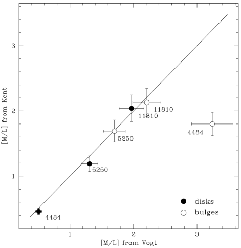
Figure 13.— A comparison of [M/L] ratios within the overlap of the sample analyzed by Kent (1986). Dark circles represent disks and open circles bulges. The deviation of the bulge of UGC4484 can be explained by different interpretations of the noncircular structure in the nuclear region and by the variation in the two luminosity profiles in the inner core within the seeing disk. The line denotes $y=x$ and error bars are plotted for a 10% error (representative of the total accuracy of the derived [M/L] ratio, not simply of the fitting technique).

Figure 13 shows the good agreement between calculated mass-to-light ratios for the overlap of this sample and that analyzed by Kent (1986). Kent’s data has been corrected to the distances and inclination angles used herein, the latter being a key factor, assuming that his inclination angle was calculated from the tabulated values of the disk eccentricity in his Table 3 and with an intrinsic axial ratio of 0.2. The data are presented in bolometric units of $\left[\frac{M_{\odot}}{L_{\odot}}\right]$ where no extinction correction has been applied (Kent’s photometric profiles are $R$-band, while ours are I-band). The deviation of the bulge of UGC 4484 can be explained by different interpretations of the noncircular structure in the nuclear region and by the variation in the two luminosity profiles in the inner core within the seeing disk (Kent quotes a seeing FWHM of 2^′′.5, versus 1″.2 herein).

7. Data Presentation

We present in Tables 2 through 4 a listing of key galaxy properties for this sample of 329 local northern hemisphere galaxies, sorted by Right Ascension. Note that quantities are not necessarily identical to similar parameters from previous publications, though no significant differences exist. A small fraction of the photometric data for the Coma cluster have been taken by combining literature results with our own measurements; specifics of those observations can be found for those sources within Giovanelli et al. 1997). Because of length, specific comments on individual galaxies are placed separately from the table, in the main text below. The data are as follows.

Table 2Galaxy Parameters I

Names	R.A.	Dec.	T	$V_{LG}$	Cluster		$r$	$s$	h-1 kpc	Qual	$\theta$
	h m s	d m s	km s-1				∘	$\sigma$	$\prime\prime$		∘
(1)	(2)	(3)	(4)	(5)	(6)	(7)	(8)	(9)	(10)	(11)	(12)
U00809/520-033	01 13 00.0	+33 33 00	5	3920	N507	f	1.54	-2.00	0.190	1311	23
U00841/502-025	01 16 22.3	+32 46 06	4	5287	N507	c	0.82	1.08	0.233	1211	54
U00927/N496	01 20 22.2	+33 16 04	4	5722	N507	c	0.22	2.06	0.233	1211	28
U00940/521-016	01 20 40.0	+34 18 30	5	6707	N507	b	1.25	4.28	0.325	1211	85
U00944/N512	01 21 10.5	+33 38 54	2	4587	N507	c	0.63	-0.50	0.233	1111	116
The complete version of this table is in the electronic edition of the Journal. The printed edition
contains only a sample.

Table 2 (Galaxy Parameters I)

Col. 1: Source identification. The first listing is an internal coding number, which is equal to the UGCnumber if the galaxy is listed in the UGCcatalog (Nilson 1973). A second galaxy name is added with the following priority scheme: if the galaxy has an NGCor ICnumber, that coding is entered preferentially; if the galaxy is listed in the CGCG(Zwicky, Herzog, & Wild 1968), that coding is listed with second priority, in the form: field number – ordinal number within the field. If entries in those three catalogs are not available, a second name is not entered.

Cols. 2 and 3: Right Ascension and Declination in the 1950 epoch; the listed positions typically have 15″ accuracy.

Col. 4: Morphological type code in the RC3 scheme, where code 1 corresponds to Sa’s, code 3 to Sb’s, and code 5 to Sc’s. The type code is followed by a “B” when the galaxy disk has an identifiable bar.

Col. 5: The galaxy radial velocity (redshift) in the CMB reference frame; this value is obtained from high quality ($Q_{HI}=1$) HI missing measurements where available, and otherwise taken from the optical spectra.

Col. 6: The cluster with which the galaxy is associated (left blank for field sources).

Col. 7: Membership code. In most cases the code consists of one of four letters: c, g, f, b,. Code c signifies that the galaxy is considered a bona fide cluster member. Code g means that the galaxy is sufficiently removed from the cluster center that cluster membership cannot be safely assigned; the galaxy is however in the periphery of the cluster, at roughly the same redshift and it is a nearby supercluster member. Codes f and b identify foreground and background galaxies respectively. The criteria adopted to arrive at the membership assignment are discussed in Paper II. In two clusters, additional codes had to be used, due to the complex nature of the structure. The Cancer group has been recognized to be an assembly of clumps, dubbed A, B, C, D (Bothun et al. 1983). We use the criteria given in that reference to assign membership to each of the clumps. The case of A2634 ($V_{LG}\sim 9200$ km s^-1) and A2666 ($V_{LG}\sim 8100$ km s^-1) is also complicated. Scodeggio et al. (1995) have produced a detailed study of the region, and within the redshift range spanned by the two clusters they also distinguished several other groups. In particular, one of the groups is at a systemic velocity near 7,000 km s^-1, near in redshift to, but distinct from A2666. We reserve the code “g7” for the members of the 7,000 km s^-1 group projected on the foreground of A2634.

Cols. 8 and 9: The angular distance $r$ in degrees and the radial separation $s$ in $\sigma$, from the center of each cluster. As the Cancer group consists of several subclumps, distances have been measured from the center of the main clump A (see Bothum et al. 1983).

Col. 10: The angular size of 1 h^-1 kpc, in arcseconds.

Col. 11: Quality and shape codes. A four digit code listing $Q_{opt}$, the quality of the optical spectra, $Q_{sh}$, the shape of the rotation curve, $Q_{{\rm HI}}$, the quality of the 21 cm line spectra, and $Q_{im}$, the quality of the $I$-band photometry.

Col. 12: The position angle $\theta$, measured eastwards from north, along which the optical spectrum was observed, in degrees.

Table 3 (Galaxy Parameters II)

Col. 1: Source identification, exactly as in Table: 2.

Cols. 2 and 3: The turnover (elbow) point and the maximum radial extent of the rotation curve R_f, in arcseconds.

Cols. 4 and 5: The differential extent of H$\alpha$ or [NII] emission, in h^-1 kpc, followed by the ratio.

Cols. 6 through 9: The measured inner and outer slopes $S_{in}$ and $S_{out}$ in normalized units, and inner and outer gradients $G_{in}$ and $G_{out}$ as a percentage of the measured optical velocity half–width, of the rotation curves (with estimated uncertainties between brackets).

Cols. 10 through 13: The velocity width from the optical spectroscopy, in km s^-1. Col. 10 lists the measured velocity width, col. 11 the velocity width corrected for the shape of the rotation curve and cosmological stretch, and col. 12 the corrected velocity width converted to edge–on viewing (with its estimated uncertainty, taking into account both measurement errors and uncertainties arising from the corrections, between brackets). Col. 13 lists the corrected velocity width converted to edge–on viewing, measured at 2 R_d.

Table 3Galaxy Parameters II

Names	Rel	Rf	$\Delta$H$\alpha$	H$\alpha_{rat}$	Sin	Sout	Gin	Gout	OW0	OW1	OW2	OW3
	$\prime\prime$	$\prime\prime$	h-1 kpc						–	km s-1		–
(1)	(2)	(3)	(4)	(5)	(6)	(7)	(8)	(9)	(10)	(11)	(12)	(13)
U00809/520-033	10.9	39.2	1.43	0.81	0.66(04)	0.10(02)	55	13	270	282	286( 6)	257( 7)
U00841/502-025	13.3	31.7	2.14	0.71	1.14(05)	0.03(06)	73	-8	247	245	249(10)	254(12)
U00927/N496	6.8	39.8	2.28	0.75	0.96(06)	0.04(01)	70	21	270	268	318(13)	318(14)
U00940/521-016	8.8	30.6	0.94	0.91	0.97(04)	0.01(01)	48	0	282	278	352( 9)	317( 8)
U00944/N512	7.7	41.0	0.96	0.90	0.83(05)	-0.01(01)	65	-10	515	500	506( 5)	510( 6)
The complete version of this table is in the electronic edition of the Journal. The printed edition contains
only a sample.

Table 4 (Galaxy Parameters III)

Col. 1: Source identification, exactly as in Table: 2.

Cols. 2 through 4: The velocity width from the 21 cm line profiles, in km s^-1. Col. 2 lists the measured velocity width, measured at a level of 50% of the profile horns, col. 3 the velocity width corrected for instrumental and data processing broadening, signal to noise effects, interstellar medium turbulence, and cosmological stretch, and col. 4 the corrected velocity width converted to edge–on viewing (with its estimated uncertainty, taking into account both measurement errors and uncertainties arising from the corrections, between brackets).

Cols. 5 through 6: The observed and the predicted HI missing masses, in units of $\log 10^{10}M_{\odot}$.

Col 7: The adopted inclination $i$ of the plane of the disk to the line of sight, in degrees, (90^∘ corresponding to edge–on perspective).

Col 8: The apparent magnitude, to which k–term, galactic and internal extinction corrections were applied, measured in Mould I.

Col 9: The absolute I magnitude, computed assuming that the galaxy is at the distance indicated either by the cluster redshift, if the galaxy is a true cluster member, or by the galaxy redshift if it is not. The calculation assumes $H_{\circ}=100h$ km s^-1 Mpc^-1, so the value listed in column 16 is strictly $M_{I}+5\log h$. In calculating this parameter, radial velocities are expressed in the LG frame and uncorrected for any cluster peculiar motion. The uncertainty on the magnitude, indicated between brackets in hundredths of a mag, is the sum in quadrature of the measurement errors and the estimate of the uncertainty in the corrections applied to the measured parameter. The error estimate does not include the uncertainty on the value of the distance.

Col 10: The disk percentage of the total luminosity.

Col 11: The disk exponential scale length, R_d, corrected to face–on value, in arcseconds.

Col 12: The radius R_23.5 at which the surface brightness profile reaches a limiting value of 23.5 magnitudes per square arcsecond, in arcseconds.

Cols 13 and 14: The stellar mass-to-light ratio, $\left[\frac{M}{L}\right]_{\star}$, in solar units. Col. 17 lists the measured $\left[\frac{M}{L}\right]_{\star}$, and col. 18 the $\left[\frac{M}{L}\right]_{\star}$ corrected for inclination and extinction effects.

Col 15: The ratio of dark to light matter, $\frac{M_{D}}{M_{L}}$, within R_f.

Comments:

AGC110759/NGC507-A1: ORC flux fairly faint.
UGC916: Use HI flux but not HI width (detection looks real, but low S/N, baseline quite sloped, horns not defined so width, systemic velocity not measurable).
UGC1045: Use TF I-band data from Han & Mould 1992; assume 2R_d lies in long, flat region of ORC.
UGC1404: Use TF I-band data from Han & Mould 1992; assume R_d = R${}_{23.5}/3.5$.
UGC1437: ORC flux suggests strong HII regions along major axis.
AGC120684: H$\alpha$ spectrum in absorption; HI profile shows wider velocity width than ORC.
AGC130014/CGCG415-058: Use TF I-band data from Han & Mould 1992; assume R_d = R${}_{23.5}/3.5$.
UGC2561: Marginal HI detection (see Magri et al. 1988); calculate HI gas mass from rms, not flux.
UGC2581: Marginal HI detection with GB300 (see Magri et al. 1988); calculate HI gas mass from rms, not flux.
UGC2617: Treat as if no HI data (clearly confused with known companion).
UGC2639: H$\alpha$ spectrum shows both emission and absorption flux.
UGC2642: Very weak H$\alpha$ emission flux; only the nucleus can be traced.
UGC2655: ORC flux suggests strong HII regions along major axis.
UGC2659: No HI data in AGC archive; use Theureau et al. 1998 (not of the same quality as our own reprocessing of archive data, because we cannot make the same corrections.)
AGC130204/CGCG540-115: H$\alpha$ spectrum quite asymmetric, with right side much fainter than left side. H$\alpha$ absorption shows faintly beyond emission; perhaps trough not completely filled?
UGC2696: H$\alpha$ absorption shows faintly beyond emission; perhaps trough not completely filled?
UGC2742: Marginal and suspect HI detection, do not use (HI profile implies much wider velocity width than ORC). Difficult to extract $H\alpha$ velocity profile due to significant $\sin(i)$ effect (very face-on).
UGC3255: Continuum extremely strong around $H\alpha$ and [NII] emission lines.
AGC150073: Gadzooks! – ORC is of neighboring galaxy (do not use).
AGC150118: ORC extremely faint, in H$\alpha$ and in [NII]. Left side less faint than right.
UGC3291: Assume that HI detection is interference peak and discard, as ORC data are solid, HI line profile shows single peak, and $\Delta$cz = 4500 km s^-1. Calculate HI gas mass from rms, not flux.
UGC4575: [NII] masked by [OH] emission line feature.
UGC4865: Inclination and corrected ellipticity from Dale et al. 1999.
UGC5250: ORC slightly truncated by edge of slit on left side.
AGC210015/A148: Irregular/ring galaxy.
AGC210643: Treat as nondetection in HI.
UGC6697: H$\alpha$ spectrum quite asymmetric and disturbed; all ORC emission lines extremely wide and strong.
UGC6718: No HI in AGC archive; use Giovanelli & Haynes 1985 (lesser quality than reprocessing of archive data).
UGC6724: Patchy HII along major axis.
UGC6746: Patchy HII along major axis.
AGC210816/CGCG127-062: Extremely faint H$\alpha$ flux, especially on right, some [NII] in nucleus.
AGC211029/F1319: Treat as if no HI data (clearly confused with known companion).
UGC6928: No HI in AGC archive; use Bottinelli et al. 1990 (lesser quality than reprocessing of archive data).
UGC7724: H$\alpha$ and [NII] spectra very weak along disk.
AGC221147/CGCG160-031: H$\alpha$ spectrum fainter on right side then on left.
UGC8069: Treat as a nondetection in HI.
UGC8096: H$\alpha$ emission line turns into strong absorption on left side.
AGC221409: [NII] extent matches H$\alpha$ extent, except on truncated side of spectrum.
UGC8161: ORC suggests patchy HII regions along major axis.
UGC8194: Use TF I-band data from Bernstein et al. 1994; assume R_d = R${}_{23.5}/3.5$.
AGC250443/CGCG049-108: Inclination and corrected ellipticity from Dale et al. 1999.
AGC250472/CGCG049-127: Inclination and corrected ellipticity from Dale et al. 1999.
AGC250632/CGCG049-151: Inclination and corrected ellipticity from Dale et al. 1999. Note $cz_{rad}=9849$ km s^-1, $cz_{orc}=9965$ km s^-1.
AGC250740/CGCG077-119: Inclination and corrected ellipticity from Dale et al. 1999.
UGC9838: No HI in AGC archive; use Freudling, Haynes & Giovanelli 1992 (lesser quality than reprocessing of archive data).
UGC9844: Inclination and corrected ellipticity from Dale et al. 1999.
AGC250803/CGCG077-126: Inclination and corrected ellipticity from Dale et al. 1999.
AGC250896/CGCG077-135: Inclination and corrected ellipticity from Dale et al. 1999.
AGC251744/CGCG476-112: Disregard HI data altogether (profile is confused with AGC251498); ORC replaced with Dale version ($\Delta$PA = $13^{\circ}$). Identified as AGC251499 in Vogt 1995.
AGC251400/CGCG108-031: Treat as if no HI data (clearly confused with known companion).
UGC10121: Inclination and corrected ellipticity from Dale et al. 1999.
AGC251424/CGCG108-037: Inclination and corrected ellipticity from Dale et al. 1999.
AGC251503: Inclination and corrected ellipticity from Dale et al. 1999.
AGC251436/CGCG108-043: Inclination and corrected ellipticity from Dale et al. 1999. ORC offset in position angle from Dale spectrum.
AGC251445/IC1157: Weak H$\alpha$ absorption, weak [NII] emission.
AGC251509: Inclination and corrected ellipticity from Dale et al. 1999.
UGC10131: ORC quite faint.
AGC251510: Inclination and corrected ellipticity from Dale et al. 1999.
UGC10166: Treat as nondetection in HI.
AGC260112/CGCG108-108: ORC offset in position angle from Dale spectrum.
AGC260116/CGCG108-107a: [NII] masked by [OH] emission line feature.
AGC260953: Disk scale length from Dale et al. 1999. H$\alpha$ on both sides, but [NII] only on the left, [NII] masked by [OH] emission line feature.
UGC10177: No HI in AGC archive; use Giovanelli & Haynes 1985 (lesser quality than reprocessing of archive data).
UGC10180: No HI in AGC archive; use Giovanelli & Haynes 1985 (lesser quality than reprocessing of archive data).
AGC260146: Inclination and corrected ellipticity from Dale et al. 1999.
UGC10190: [NII] masked by [OH] emission line feature.
UGC10192: Identified as AGC260184 in Vogt 1995. No HI in AGC archive; use Huchtmeier & Richter 1989 (lesser quality than reprocessing of archive data).
UGC10193: [NII] masked by [OH] emission line feature. Note moderately close companion in ORC ($\Delta$cz = 600 km s^-1) and in I-band.
UGC10195: No HI in AGC archive; use Giovanelli & Haynes 1985 (lesser quality than reprocessing of archive data).
AGC260208/CGCG108-140: Inclination and corrected ellipticity from Dale et al. 1999.
AGC260226/IC1192: Inclination and corrected ellipticity from Dale et al. 1999.
AGC260245: Inclination and corrected ellipticity from Dale et al. 1999. H$\alpha$ beyond [NII] is very faint on left, bright on right.
AGC260246/CGCG108-155: Inclination and corrected ellipticity from Dale et al. 1999.
AGC260274/CGCG108-157: H$\alpha$ outlying points on left are quite faint.
UGC10287: ORC offset in position angle from Dale spectrum.
UGC10389: No HI in AGC archive; use Huchtmeier & Richter 1989 (lesser quality than reprocessing of archive data).
AGC260599: ORC very probably has large position angle offset (do not use velocity profile).
UGC10415: Face-on galaxy, ORC is quite noisy because of inclination angle factor, major axis was difficult to determine.
AGC260929: Faint, patchy HII along major axis.
AGC260622: Faint, patchy HII along major axis.
AGC260930: Fairly strong H$\alpha$ emission spectrum, but [NII] extremely faint.
AGC260934: [NII] masked by [OH] emission line feature.
UGC10661:Use HI flux but not width (detection looks real, but low S/N, horns not defined).
UGC11348: No HI data in AGC archive; use Theureau et al. 1998 (lesser quality than reprocessing of archive data).
AGC330564/CGCG476-075: Strong, solid body inner ORC profile rises above V_max - bar?
AGC330712: Strong H$\alpha$, but no [NII] to trace along ORC.
UGC12721: Patchy HII along disk (isolated points appear to be real, match I-band).
AGC330721: Treat as if no HI data; likely confused with known companion.
AGC330768/CGCG476-112: Sole case of strong ORC asymmetry outside of cluster cores, from interacting neighbor at 16 h^-1 kpc.
AGC331185/F2532: New AGC name for AGC331096 (deactivated). HI spectrum has been published as AGC331096, and recorded in NED. Identified as AGC331096 in Vogt 1995.
AGC330918/CGCG498-012: Use TF I-band data from Han & Mould 1992; assume R_d = R${}_{23.5}/3.5$.
AGC330958/CGCG477-020: HI marginal (S/N barely acceptable) and $\Delta$cz = 1200 km s^-1 from ORC; assume nondetection in HI and calculate HI gas mass from rms, not flux.
AGC331013/CGCG478-003: HI marginal (S/N barely acceptable) and $\Delta$cz = 200 km s^-1 from ORC; assume nondetection in HI and calculate HI gas mass from rms, not flux.

Table 4Galaxy Parameters III

Names	$RW_{0}$	$RW_{1}$	$RW_{2}$	$M_{HI}(obs,exp)$		$i$	$I$	$M_{I}$	D/T	Rd	$R_{23.5}$	$\left[\frac{M}{L}\right]$		$\frac{M_{D}}{M_{L}}$
	–	km s-1	–	$\log 10^{10}M_{\odot}$		∘			%	$\prime\prime$	$\prime\prime$	$\odot$
(1)	(2)	(3)	(4)	(5)	(6)	(7)	(8)	(9)	(10)	(11)	(12)	(13)	(14)	(15)
U00809/520-033	314	289	291( 6)	9.31	9.25	83	13.55	-22.30(03)	98	10.32	49.5	0.64	2.06	0.15
U00841/502-025	290	262	266( 8)	9.27	9.54	80	13.58	-22.18(03)	97	8.90	43.5	0.62	1.71	0.13
U00927/N496	297	271	322(12)	9.72	9.61	57	12.47	-22.93(05)	97	14.77	52.3	1.07	1.61	0.08
U00940/521-016	288	260	331(13)	9.57	9.48	52	13.63	-22.43(04)	93	8.77	30.5	1.71	2.42	0.19
U00944/N512	522	493	499( 7)	9.41	9.36	81	12.04	-23.70(02)	91	8.70	55.4	0.50	1.30	0.28
The complete version of this table is in the electronic edition of the Journal. The printed edition contains only a
sample.

Figure 14 presents the data on the derived rotation curves for the entire sample of galaxies, sorted by right ascension and labeled by AGC name. Filled circles designate the H$\alpha$ data, and open circles the [NII] data (where traced). Error bars are plotted only on points for which they have an amplitude greater than 10 km s^-1, to reduce obscuration of the points. The x-axis shows the radial distance along the major axis in units of h^-1 kpc, and the y-axis the velocity in units of km s^-1. The cluster name is added for galaxies within 2 h^-1 Mpc of a cluster center, and the galaxy radius (h^-1 Mpc) and velocity offset ($\sigma$) are below. The absolute magnitude M_I is then added for all galaxies as available. For galaxies within 1 h^-1 Mpc of a cluster center, an arrow at the center of the rotation curve points in the direction of the cluster center. (The angle between the x-axis and the arrow indicates the position of the major axis relative to the cluster center, the angle between the rotation curve, showing the velocity along the major axis, and the arrow means nothing.)

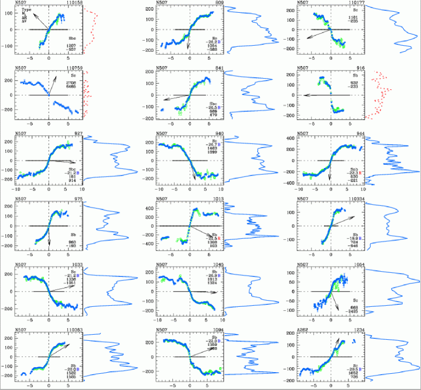
Figure 14.— Rotation curves are shown for the entire sample, sorted by right ascension and labeled by AGC name. Filled blue circles show H$\alpha$ data, and open green circles [NII] data; error bars are plotted when larger than 10 km s^-1. The x-axis shows the radial distance along the major axis, in h^-1 kpc, and the y-axis the velocity, in km s^-1. The cluster name is noted for galaxies within two h^-1 Mpc of a cluster center, with the galaxy radius (h^-1 Mpc) and velocity offset ($\sigma$) inset below the morphological type. The absolute magnitude M_I and $B-I$ color (B/R) are added if available. A solid $\pm 2R_{d}$ disk length is drawn along the major axis. For galaxies within one h^-1 Mpc of a cluster center, an arrow from the center of the rotation curve points towards the cluster center (the angle between the x-axis and the arrow indicates the position of the major axis relative to the cluster center.) To the right of each rotation curve we present the HI missing line profile, preserving the velocity scale on the y-axis. The blue line profiles are scaled along the x-axis to fill the available horizontal space rather than in absolute flux units, but the line profile is scaled lower and drawn as a dotted red line for galaxies which are HI missing deficient by more than a factor of 2.5 (log HI missing ${}_{def}\geq$ 0.40). [The complete version of this figure is in the electronic edition of the Journal. The printed edition contains only a sample.]

To the right of each rotation curve we present the HI missing line profile, preserving the velocity scale on the y-axis to allow a comparison of the HI missing flux distribution with the rotation curve as a function of radius. The line profile is scaled along the x-axis to fill the available space rather than in absolute flux units, but the line profile is drawn with a dotted line for galaxies which are HI missing deficient by more than a factor of 2.5 (log HI missing ${}_{def}\geq$ 0.40).

Figure 15⁴ shows the rotation curves folded about their centerpoints for the galaxies for which we have $I$-band data, sorted by right ascension and labeled by AGC name. Circles designate the H$\alpha$ data, and triangular points the [NII] data, while filled points and empty points fall respectively on the approaching and receding sides of the source. Error bars are again plotted only on points for which they have an amplitude greater than 10 km s^-1, to reduce obscuration of the points. The x-axis shows the radial distance along the major axis in units of h^-1 kpc, and the y-axis the velocity in units of km s^-1. For sources where an image is available and thus an inclination angle is known, the profiles have been corrected by $\sin(i)$ to edge–on amplitude. Maximum disk mass models have been superimposed on top of the rotation curves for sources for which images are available. The dotted lines represent the bulge components, the dot-long-dashed lines the disk components, the dot-short-dashed lines the halo components, and the solid lines the total velocity models. The component profiles have been terminated at the end of the luminosity profile for the few sources in which the optical rotation curve extends further out than the traced luminosity profile. The upright arrows placed upon the x–axis mark one disk scale length.

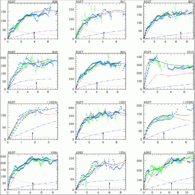
Figure 15.— Rotation curves are folded about their centerpoints for the galaxies for which we have $I$-band data, sorted by right ascension and labeled by AGC name. Solid blue circles designate the H$\alpha$ data, and the open green circles the [NII] data. Error bars are again plotted when larger than 10 km s^-1. The x-axis shows the radial distance along the major axis, in units of h^-1 kpc, and the y-axis the velocity, in units of km s^-1. The profiles have been corrected by $\sin(i)$ to edge–on amplitude. Maximum disk mass models have been superimposed on top of the rotation curves; the dotted purple lines represent the bulge components, the dot-long-dashed red lines the disk components, the dot-short-dashed blue lines the halo components, and the solid black lines the total velocity models. Upright arrows on the x–axis mark one disk scale length. [The complete version of this figure is in the electronic edition of the Journal. The printed edition contains only a sample.]

Figure 16⁴ presents the data on the $I$-band surface brightness profiles for the galaxies within the rotation curve sample for which we have such data, sorted by right ascension and labeled by AGC name. The x-axis shows the radial distance along the major axis in h^-1 kpc, and the y-axis the surface brightness profile, azimuthally averaged along the fitting ellipse, in magnitudes per square arcsecond. A an arrow marks the radius of two disk scale lengths, and the bulge and disk components have been deconvolved.

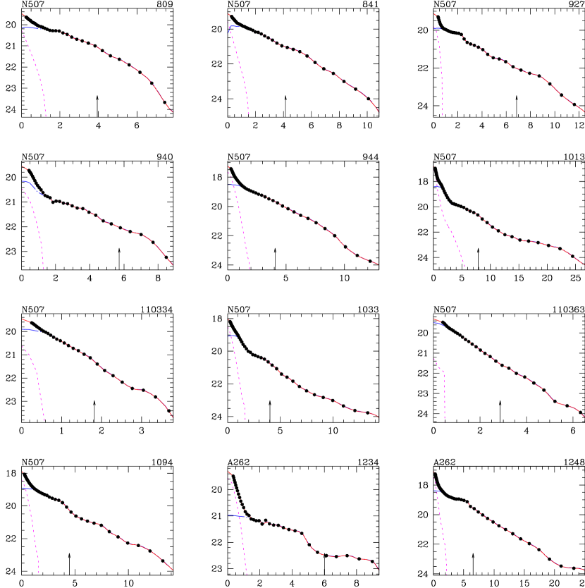
Figure 16.— $I$-band surface brightness profiles are drawn for the galaxies for which we have $I$-band data, sorted by right ascension and labeled by AGC name. The x-axis shows the radial distance along the major axis, in h^-1 kpc, and the y-axis the surface brightness profile (red), azimuthally averaged along the fitting ellipse, in magnitudes per square arcsecond. An arrow marks the radius of two disk scale lengths, and the bulge (purple) and disk (blue) components have been deconvolved. [The complete version of this figure is in the electronic edition of the Journal. The printed edition contains only a sample.]

8. Summary

This study concerns the effects of the cluster environment upon the distribution of mass and light in spiral galaxies. We have observed a set of 329 nearby (redshift $z<0.045$) galaxies, (1) to study the dependence of mass–to–light distributions upon cluster environment, (2) to evaluate the global properties of optical rotation curves (spatially extended velocity profiles), and (3) to determine the robustness of the Tully–Fisher relation within differing environments. The 16 Abell clusters cover a wide range of cluster richness, density, and luminosity, and are supplemented by the less rich groups Cancer and NGC507, and 30 isolated field galaxies. We have examined the distribution of mass and light within the target galaxies through a study of optical emission lines, the total HI missing gas, and optical photometry. Optical spectroscopy were taken with the 200-inch Hale Telescope and provide separately resolved H$\alpha$ and [NII] major axis rotation curves for the complete set of galaxies, which are analyzed to yield velocity widths and velocity profile shapes and gradients. HI missing line profiles provide an independent velocity width measurement and a measure of HI missing gas deficiency. $I$-band images are used to deconvolve profiles into disk and bulge components and to determine global luminosities and inclination. This paper is the first in a series of three linked papers concerning this data set. The present paper (Paper I) covers the observational data collected; the remaining two (Vogt et al. 2003; Paper II and Paper III) contain the results of the analysis of cluster properties and environmental effects.

9. Acknowledgments

The data presented in this paper are based upon observations carried out at the Arecibo Observatory, which is part of the National Astronomy and Ionosphere Center (NAIC), at Green Bank, which is part of the National Radio Astronomy Observatory (NRAO), at the Kitt Peak National Observatory (KPNO), the Palomar Observatory (PO), and the Michigan–Dartmouth–MIT Observatory (MDM). NAIC is operated by Cornell University, NRAO by Associated Universities, inc., KPNO and CTIO by Associated Universities for Research in Astronomy, all under cooperative agreements with the National Science Foundation. The MDM Observatory is jointly operated by the University of Michigan, Dartmouth College and the Massachusetts Institute of Technology on Kitt Peak mountain, Arizona. The Hale telescope at the PO is operated by the California Institute of Technology under a cooperative agreement with Cornell University and the Jet Propulsion Laboratory. We would like to thank the staff members at these observatories who so tirelessly dedicated their time to insure the success of our observations. We also thank Sc project team members John Salzer, Gary Wegner, Wolfram Freudling, Luiz da Costa, and Pierre Chamaraux, and also Shoko Sakai and Marco Scodeggio, for sharing their data in advance of publication. We thank the anonymous referee for helpful comments on the manuscript.

N.P.V. is a Guest User, Canadian Astronomy Data Center, which is operated by the Dominion Astrophysical Observatory for the National Research Council of Canada’s Herzberg Institute of Astrophysics. This research has made use of the NASA/IPAC Extragalactic Database (NED) which is operated by the Jet Propulsion Laboratory, California Institute of Technology, under contract with NASA. This research was supported by NSF grants AST92–18038 and AST95–28860 to M.P.H. and T.H., AST90–23450 to M.P.H., AST94–20505 to R.G., and NSF–0123690 via the ADVANCE Institutional Transformation Program at NMSU, and NASA grants GO-07883.01-96A to N.P.V. and NAS5–1661 to the WFPC1 IDT.

References

- (1)
- (2) Abell, G. O., Corwin, H. G., Jr., & Olowin, R. P. 1989, ApJS, 70, 1
- (3) Adami, C.; Marcelin, M., Amram, P., Russeil, D. 1999, A&A, 349, 812
- (4) Amram, P., Balkowski, C., Boulesteix, J., Cayatte, V., Marcelin, M., & Sullivan, W. T., III 1996, A&A, 310, 737
- (5) Amram, P., Marcelin, M., Balkowski, C., Cayatte, V., Sullivan, W. T., III, & Le Coarer, E. 1994, A&AS, 103, 5
- (6) Amram, P., Sullivan, W. T., III, Balkowski, C., Marcelin, M., & Cayatte, V. 1993, ApJ, 403, L59
- (7) Amram, P., Le Coarer, E., Marcelin, M., Balkowski, C., Sullivan, W. T., III, & Cayatte, V. 1992, A&AS, 94, 175
- (8) Beers, T. C., Gebhardt, K., Forman, W., Huchra, J. P., & Jones, C. 1991, AJ, 102, 1581
- (9) Bernstein, G. M., Guhathakurta, P., Raychaudhury, S., Giovanelli, R., Haynes, M. P., Herter, T., & Vogt, N. P. 1994, AJ, 107, 1962
- (10) Bosma, A. 1978, Ph.D. thesis, University of Groningen
- (11) Bothun, G. D., Geller, M. J., Beers, T. C., & Huchra, J. P. 1983, ApJ, 268, 47
- (12) Bottinelli, L., Gouguenheim, L., Fouqué, P., & Paturel, G. 1990, A&AS, 82, 391
- (13) Burstein, D., Rubin, V. C., Ford, W. K., & Whitmore, B. C. 1986, ApJ, 305, L11
- (14) Burstein, D., & Rubin, V. C. 1985, ApJ, 297, 423
- (15) Burstein, D., Rubin, V. C., Thonnard, N., & Ford, W. K. 1982, ApJ, 253, 70
- (16) Corradi, R. L. M. & Capaccioli, M. 1991, A&AS, 90, 121
- (17) Courteau, S. 1997, AJ, 114, 2402
- (18) Courteau, S. 1992, Ph.D. thesis, University of California, Santa Cruz
- (19) Dale, D. A., Giovanelli, R. Haynes, M. P., Scodeggio, M., Hardy, E., & Campusano, L. E. 1997, AJ, 114, 455
- (20) Dale, D. A., Giovanelli, R. Haynes, M. P., Scodeggio, M., Hardy, E., & Campusano, L. E. 1999, AJ, 115, 418
- (21) Dale, D. A., Giovanelli, R. Haynes, M. P., Hardy, E., & Campusano, L. E. 1999, AJ, 118, 1486
- (22) Distefano, A., Rampazzo, R., Chincarini, G., & de Souza, R. 1990, A&AS, 86, 7
- (23) Dressler, A. 1980, ApJS, 42, 565
- (24) Faber, S. M., & Gallagher, J. S. 1979, ARA&A, 17, 135
- (25) Forbes, D. A., & Whitmore, B. C. 1989, ApJ, 339, 657
- (26) Freeman, K. C. 1970, ApJ, 160, 811
- (27) Freudling, W., Haynes, M. P., & Giovanelli, R. 1992, ApJS, 79, 157
- (28) Freudling, W., Haynes, M. P., & Giovanelli, R. 1988, AJ, 96, 1791
- (29) Garrido, O., Marcelin, M., Amram, P., & Boulesteix, J. 2002, A&A, 387, 821
- (30) Garrido, O., Marcelin, M., Amram, P., & Boissin, O. 2003, A&A, 399, 51
- (31) Giovanelli, R., & Haynes, M. P. 1985, ApJ, 292, 404
- (32) Giovanelli, R., & Haynes, M. P. 2002, ApJ, 571, L107
- (33) Giovanelli, R., Haynes, M. P., Herter, T., Vogt, N. P., Wegner, G., Salzer, J. J., da Costa, L. N., & Freudling, W. 1997, AJ, 113 22
- (34) Giovanelli, R., Haynes, M. P., Salzer, J. J., Wegner, G., da Costa, L., & Freudling, W. 1995, AJ, 110 1059
- (35) Giovanelli, R., Haynes, M. P., Salzer, J. J., Wegner, G., da Costa, L., & Freudling, W. 1994, AJ, 107, 2036
- (36) Giovanelli, R., Chincarini, G. L., & Haynes, M. P. 1981, ApJ, 247, 383
- (37) Guhathakurta, P., van Gorkom, J. H., Kotanyi, C. G., & Balkowski, C. 1988, AJ, 96, 851
- (38) Gunn, J. E., & Gott, J. R., III, 1972, ApJ, 176, 1
- (39) Han, M. 1992, ApJ, 395, 75
- (40) Han, M., & Mould, J. 1992, ApJ, 396, 453
- (41) Haynes, M. P., Giovanelli, R., Salzer, J. J., Wegner, G., Freudling, W., da Costa, L. N., Herter, T., & Vogt, N. P. 1999, AJ, 117, 1668
- (42) Haynes, M. P., Giovanelli, R., Herter, T., Vogt, N. P., Freudling, W., Maia, M. A. G., Salzer, J. J., & Wegner, G. 1997, AJ, 113, 1197
- (43) Haynes, M. P. 1989, NAIC Bul., 254, 1
- (44) Haynes, M. P., Magri, C., & Giovanelli, R. 1988, AJ, 95, 607
- (45) Haynes, M. P., & Giovanelli, R. 1986, ApJ, 306, 466
- (46) Haynes, M. P., & Giovanelli, R. 1984, AJ, 89, 758
- (47) Huchtmeier, W. K., & Richter, O.-G. 1989, A&A, 210, 1
- (48) Kent, S. M. 1986, AJ, 91, 1301
- (49) Kogut, A., et al. 1993, ApJ, 419, 1
- (50) Lewis, B. M. 1980, in preparation
- (51) Magri, C., Haynes, M. P., Forman, W., Jones, C., & Giovanelli, R. 1988, ApJ, 333, 136
- (52) Mathewson, D. S., Ford, V. L., & Buchhorn, M. 1992, ApJS, 81, 413
- (53) Mathewson, D. S. & Ford, V. L. 1996, ApJS, 107, 97
- (54) Neistein, E., Maoz, D., Rix, H.-W., & Tonry, J. L. 1999, AJ, 117, 2666
- (55) Nilson, P. 1973, Uppsala General Catalogue of Galaxies (Uppsala: Astronomiska Observatorium) (UGC)
- (56) Oke, J. B., & Gunn, J. E. 1982, PASP, 94, 586
- (57) Persic, M., & Salucci, P. 1990, MNRAS, 245, 577
- (58) Rix, H.-W., Guhathakurta, P., Colless, M., & Ing, K. 1997, MNRAS, 285, 779
- (59) Rowan–Robinson, M. 1977, Cosmology, (Oxford: Clarendon Press)
- (60) Rubin, V. C., Ford, W. K., & Whitmore, B. C. 1988, ApJ, 333, 522
- (61) Rubin, V. C., Burstein, D., Ford, W. K., & Thonnard, N. 1985, ApJ, 261, 439
- (62) Rubin, V. C., Ford, W. K., Jr., Thonnard, N., & Burstein, D. 1982, ApJ, 289, 81
- (63) Rubin, V. C., Ford, W. K., Jr., & Thonnard, N. 1980, ApJ, 238, 471
- (64) Scodeggio, M., Solanes, J. M., Giovanelli, R., & Haynes, M. P. 1995, ApJ, 444, 41
- (65) Solanes, J. M., Giovanelli, R., & Haynes, M. P. 1996, ApJ, 461, 609
- (66) Solanes, J. M., Manrique, A., García-Gómez, C., González-Casado, G., Giovanelli, R., & Haynes, M. P. 2001, ApJ, 548, 97
- (67) Sperandio, M., Chincarini, G., Rampazzo, R., & de Souza, R. 1995, A&AS, 110, 279
- (68) Theureau, G.. et al. 1998, A&AS, 130, 333
- (69) Toomre, A., & Toomre, J. 1972, ApJ, 178, 623
- (70) Tully, R. B., & Fisher, J. R. 1977, A&A, 54, 661
- (71) Vogt, N. P., Haynes, M. P., Giovanelli, R., & Herter, T. 2004a, ApJ, in press (Paper II)
- (72) Vogt, N. P., Haynes, M. P., Giovanelli, R., & Herter, T. 2004b, ApJ, in press (Paper III)
- (73) Vogt, N. P. 1995, Ph.D. thesis, Cornell University
- (74) Weinberg, M. 1996, ApJ, 478, 435
- (75) Whitmore, B. C., Forbes, D. A., & Rubin, V. C. 1988, ApJ, 333, 542
- (76) Zwicky, F., Herzog, E., & Wild, P. 1961 - 1968, Catalogue of Galaxies and of Clusters of Galaxies, I - VI (Pasadena: California Institute of Technology) (CGCG)