Comprehensive analysis of $RGU$ photometry in the direction to M5

Abstract

The $RGU$-photographic investigation of an intermediate latitude field in the direction to the Galactic center is presented. 164 extra-galactic objects, identified by comparison of Minnesota and Basel charts, are excluded from the program. Also, a region with size 0.104 square-degrees, contaminated by cluster (M5) stars and affected by background light of the bright star HD 136202 is omitted. Contrary to previous investigations, a reddening of $E(B-V)=0.046$, corresponding to $E(G-R)=0.07$ mag is adopted. The separation of dwarfs and evolved stars is carried out by an empirical method, already applied in some of our works. A new calibration for the metallicity determination is used for dwarfs, while the absolute magnitude determination for stars of all categories is performed using the procedures given in the literature. There is good agreement between the observed logarithmic space density histograms and the galactic model gradients. Also, the local luminosity function agrees with Gliese’s (1969) and Hipparcos’ (Jahreiss & Wielen 1997) luminosity functions, for stars with $2<M(G)\leq 8$ mag. For giants, we obtained two different local space densities from comparison with two Galactic models, i.e. $D^{*}(0)=6.63$, close to that of Gliese (1969), and $D^{*}(0)=6.79$. A metallicity gradient, $d[Fe/H]/dz=-0.20$ dex/kpc, is detected for dwarfs (only) with absolute magnitudes $4<M(G)\leq 6$, corresponding to a spectral type interval F5-K0.

¹ Istanbul University Science Faculty, Department of Astronomy and Space Sciences, 34452 University- Istanbul, Turkey
karsa@istanbul.edu.tr
sbilir@istanbul.edu.tr
² Astronomisches Institut der Universität Basel, Venusstr. 7, 4102 Binningen, Switzerland
Roland.Buser@unibas.ch

Keywords: Galaxy: structure – Galaxy: metallicity gradient – Stars: luminosity function

1 Introduction

The photographic data presented in this paper have been obtained in the context of the re-evaluation program of the Basel $RGU$ three-colour photometric high-latitude survey of Galaxy, which comprises homogeneous magnitudes and colours for about 20000 stars in a total of fourteen fields distributed along the Galactic meridian through the Galactic center and the Sun (Buser & Rong 1995). The main purpose of the present investigation of this field near M5 is to check the possible metallicity gradient, claimed by many researchers (cf.Reid & Majewski 1993, Chiba & Yoshii 1998). This can be carried out employing known solar neighbourhood constraints, especially with consistency of the local stellar luminosity function. Thus, all methodical tools have been used to obtain a stellar luminosity function agreeable with that of Gliese (1969) and Hipparcos (Jahreiss & Wielen 1997), as explained in the following sections. In Section 2, we describe the identification of extra-galactic objects, the contamination with cluster stars, the background effect of the bright star HD 136202, and the two-colour diagrams. Section 3 is devoted to the separation of evolved stars (sub-giants and giants) and dwarfs, and the determination of absolute magnitudes and metallicities. The evaluation of density and luminosity functions is given in Section 4. In Section 5, the metallicity distribution is discussed and in Section 6, we provide a summary and brief discussion.

2 The data

2.1 Extra-galactic objects, cluster stars, stars affected by background light, and stars absent on Minnesota charts

The comparison of Basel and Minnesota charts revealed that there is a considerable number of extra-galactic objects in the star fields, which cause an excess in the density and luminosity functions (Bilir et al. 2003). Hence, we applied the same procedure to eliminate such objects in our field. It turned out that 164 sources are extra-galactic objects, i.e. quasars or galaxies, occupying different regions in the two-colour diagrams (Fig.1). All these objects have been excluded from the program. Also, comparison of the number of stars per square-degree in the vicinity of the cluster M5 ($l=4^{o}.0$, $b=+47^{o}.0$, size 1.05 square-degrees) and at relatively farther distances revealed that the field is contaminated by cluster stars, causing a similar effect as just cited above. Additionally, some stars are affected by background light of the bright star HD 136202 ($\alpha=15^{h}~{}19^{m}~{}18^{s}.80$, $\delta=+01^{o}~{}45{{}^{\prime}}~{}55{{}^{\prime\prime}}.5$) in our field. To avoid such an effect a region with size 0.104 square-degrees was excluded from the field (Fig.2). Finally 33 objects which do not appear on either the Basel or the Minnesota charts have been omitted. Hence, a total number of 1368 stars have been included in the analysis within the limiting apparent magnitude $G=18.5$ and within the field of size $0.954$ square-degrees.

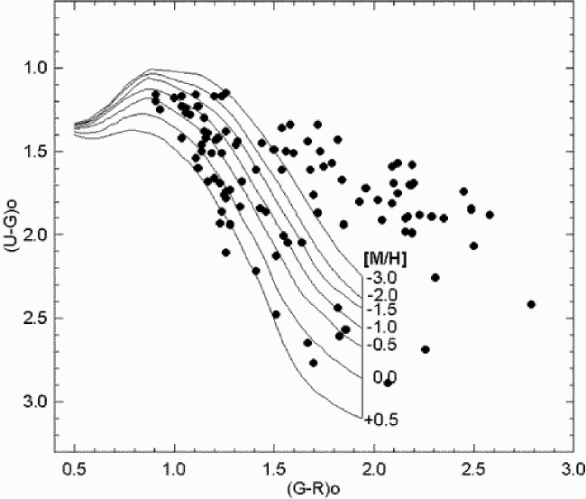
Figure 1: Extra-galactic objects identified by comparison of Minnesota and Basel charts. Their number within the limiting apparent magnitude, $G=18.5$, is 104, but increases up to 164 when counted down to the faintest object in the Basel catalogue.

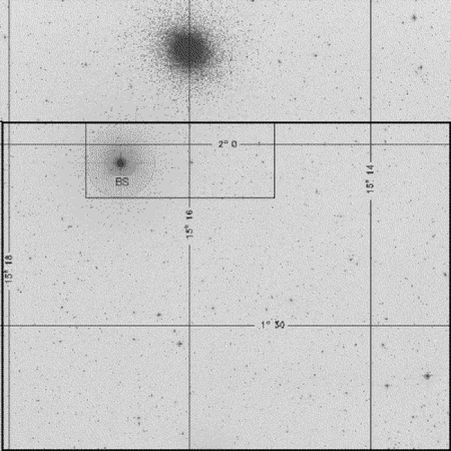
Figure 2: The field chart showing the position of the cluster M5, the bright star HD 136202 ($\alpha=15^{h}~{}19^{m}~{}18^{s}.80$, $\delta=+01^{o}~{}45{{}^{\prime}}~{}55{{}^{\prime\prime}}.5$), labelled with BS, and the surrounding excluded area of 0.104 square-degrees. The horizontal and vertical axes give the right ascension ($\alpha$) and declination ($\delta$), respectively.

2.2 $RGU$ magnitudes, interstellar reddening, and two-colour diagrams

The measurements, carried out by an automatic plate measuring machine (COSMOS) in 1980s in Edinburgh Royal Observatory, are transformed to the $RGU$-system according to Buser’s (1978) formulae, with the help of 26 photoelectric $UBV$-standards. Although zero reddening was adopted in former investigations of this field (Becker et al. 1978, Fenkart & Karaali 1990, Buser et al. 1998; 1999), we adopted the $E(B-V)=0.046$ cited by Schlegel et al. (1998), which corresponds to $E(G-R)=0.07$ mag in Buser’s system. The resulting extinction of this reddening is $A(G)=2.7E(G-R)=0.19$ mag. Thus, all colours and magnitudes used in this work are de-reddened. We fixed the limiting apparent magnitude at $G=18.5$, and omitted stars fainter than this magnitude (Fig.3).

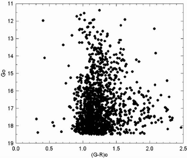
Figure 3: Colour-magnitude diagram for the field down to the limiting magnitude, $G=18.5$.

Figure 4: Two-colour diagrams in consecutive apparent magnitude intervals, i.e. (a) $G\leq 14.0$, (b) $14.0<G\leq 15.0$, (c) $15.0<G\leq 16.0$, (d) $16.0<G\leq 16.5$, (e) $16.5<G\leq 17.0$, (f) $17.0<G\leq 17.5$, (g) $17.5<G\leq 18.0$, and (h) $18.0<G\leq 18.5$. The superposed grid of iso-metallicity lines for dwarf stars is based on theoretical model atmosphere calculations (Buser & Fenkart 1990). Symbols: ($\bullet$) dwarf, (x) evolved, (O) untreated, and (+) extra-galactic objects.

The total number of stars in the sample is 1368. Their numbers in each panel on Fig.4 are given in Table 1 together with the numbers of extra-galactic objects. The two-colour diagrams given in consecutive apparent magnitude intervals (Fig.4) is typical for an intermediate latitude field in the center direction of the Galaxy, i.e. most of the stars lie in the regions occupied by metal-rich or intermediately metal-rich stars, whereas the metal-poor stars are rare. Also, the scattering is less when compared with our recent works (cf. Karataş et al. 2001). Though, there are 262 stars which occupy the metallicity regions $[Fe/H]>+0.5$ dex or $[Fe/H]<-3$ dex where, usually, stars do not exist or they are rather sparse. Hence, these stars were excluded from the program without any inquiring. However, most of them (206) are relatively faint ones, $G>17.0$ mag, therefore they may be undetected blended stars. The exclusion of these extreme stars do not affect the metallicity distribution (see Section 6). Additionally, as they lie in a large range of the colour-index $(G-R)_{o}$ almost uniformly (Fig.4), they attribute to different $M(G)$ absolute magnitudes. Hence, they do not affect the luminosity function (see Section 4, Fig.7) either.

Table 1: Number of stars and extra-galactic objects within the limiting magnitude $G=18.5$ for different panels in Fig.4.

Panel	Apparent	Number of	Number of
	magnitude	stars	extra-galactic objects
Fig.4a	$~{}~{}~{}~{}~{}~{}~{}~{}~{}~{}G\leq 14.0$	85	3
Fig.4b	$14.0<G\leq 15.0$	96	3
Fig.4c	$15.0<G\leq 16.0$	154	11
Fig.4d	$16.0<G\leq 16.5$	141	7
Fig.4e	$16.5<G\leq 17.0$	157	11
Fig.4f	$17.0<G\leq 17.5$	220	13
Fig.4g	$17.5<G\leq 18.0$	258	28
Fig.4h	$18.0<G\leq 18.5$	257	28
	Total	1368	104

3 Separation of evolved stars, metallicity and absolute magnitude determination

Following our recent experiences (Karaali 1992, Karaali et al. 1997, Ak et al. 1998 Karataş et al. 2001, and Karaali et al. 2003), for apparent magnitudes brighter than $G=17$, stars which according to their positions in the two-colour diagram could be identified as dwarfs with assigned absolute magnitudes fainter than $M(G)=6$ (but see Section 4), are most likely evolved sub-giant or giant stars with correspondingly brighter absolute magnitudes, and their metallicities and absolute magnitudes are determined by the procedure given by Buser et al. (2000). Metallicities for dwarfs were determined using a new calibration, similar to that of Carney (1979), i.e. $[Fe/H]=0.11-2.22\delta-7.95\delta^{2}$, where $\delta$ is the ultra-violet excess at $G-R=1.08$ mag, corresponding to $B-V=0.60$ mag (Karaali & Bilir 2002, see Appendix), and their absolute magnitudes are determined by means of the colour-magnitude diagrams of Buser & Fenkart (1990). The scale of the new metallicity calibration, $-2.20\leq[Fe/H]\leq+0.20$ dex, is large enough to cover most of the dwarfs in our field. Actually, the number of dwarfs whose metallicities lie out of this interval is not large, so does not affect the metallicity distribution (see Section 5).

4 Density and luminosity functions

The logarithmic space densities $D^{*}=logD(r)+10$ for stars of all population types, i.e. Population I (thin disk), Intermediate Population II (thick disk), and Extreme Population II (halo) are given in Tables 2 and 3, for dwarfs and sub-giants, and giants, respectively. Here, $D=N/\Delta V_{1,2}$, N being the number of stars, found in the partial volume $\Delta V_{1,2}$, which is determined by the limiting distances $r_{1}$ and $r_{2}$, and apparent field size in square degrees $\Box$, i.e. $\Delta V_{1,2}=(\pi/180)^{2}(\Box/3)(r_{2}^{3}-r_{1}^{3})$. As usual, density functions are then given in the form of histograms with density plotted as a solid dot at the centroid distance, $\bar{r}=[(r^{3}_{1}+r^{3}_{2})/2]^{1/3}$, of the corresponding volume, $\Delta V_{1,2}$ (see, e.g., Del Rio & Fenkart 1987, and Fenkart & Karaali 1987).

The comparison of the density functions with the best fitting model gradients predicted by Buser, Rong, & Karaali (BRK 1998, 1999) and by Gilmore & Wyse (GW 1985) are matched to the observed profiles in order to extrapolate the local stellar space densities. In both works the model gradients for thin disk and thick disk are calculated from the double exponentials fitted to them, whereas for halo the de Vaucouleurs spheroid is used for this purpose. The model gradients compared with the observed density functions are the combined ones for three galactic components, i.e. thin disk, thick disk, and halo. A small disagreement between the observed data and both models was noticed only for two absolute magnitude intervals, i.e. the excess number of stars with $5<M(G)\leq 6$ within the distance interval $1.59<r\leq 3.98$ kpc and the deficient number of stars with $3<M(G)\leq 4$ beyond the distance $r=3.98$ kpc. Assuming that about 60 stars in the fainter absolute magnitude interval are evolved leads to observed densities near the predicted model gradients for both absolute magnitude intervals, i.e. $3<M(G)\leq 4$ and $5<M(G)\leq 6$. Most of the stars cited above turned out to be with absolute magnitudes $3<M(G)\leq 4$, and about a dozen of them with $4<M(G)\leq 5$ mag. Their apparent magnitudes are fainter than $G=16$, however the peak of their magnitude distribution lies at $G\cong 17.5$ mag Tables 2 and 3 give the final results.

Thus, we obtain good agreement between the gradients for both models, BRK and GW, and the observed logarithmic space density histograms (Fig.5 and Fig.6). The same holds also for the local densities, except for the giants, as explained as follows: the stellar luminosity function resulting from comparison of observed histograms with the best fitting BRK- and GW-model gradients agrees with the Gliese’s (1969) and Hipparcos’ (JW 1997) luminosity functions for all absolute magnitude intervals, i.e. $2<M(G)\leq 3$, $3<M(G)\leq 4$, $4<M(G)\leq 5$, $5<M(G)\leq 6$, $6<M(G)\leq 7$, and $7<M(G)\leq 8$ (Fig.7). However, two different local densities are obtained for giants. Comparison with the GW model can be carried out up to the limiting distance of completeness, $r=15.85$ kpc, corresponding to a height of $z=11.59$ kpc from the Galactic plane, and gives a local density of $D^{*}(0)=6.63$, rather close to Gliese’s (1969) value, $\odot=6.64$. At this distance the observed density falls abruptly and diverges from these model gradients for larger distances. On the other hand, for the model gradients from BRK, the comparison up to $r=15.85$ kpc gives a local density $D^{*}(0)=6.79$, and the agreement holds up to the distance $r=19.95$ kpc with a local density slightly different from the previous one, $D^{*}(0)=6.77$.

Table 2: The logarithmic space densities $D^{*}=logD+10$ for dwarfs and sub-giants of all population types, where $D=N/\Delta V_{1,2}$, N being the number of stars found in the partial volume $\Delta V_{1,2}$, determined by the limiting distances $r_{1}$ and $r_{2}$, and apparent field size in square degrees $\Box$, i.e. $\Delta V_{1,2}=(\pi/180)^{2}(\Box/3)(r_{2}^{3}-r_{1}^{3})$. $\bar{r}$: centroid distance $\bar{r}=[(r^{3}_{1}+r^{3}_{2})/2]^{1/3}$, of the corresponding volume, $\Delta V_{1,2}$, heavy horizontal lines: limiting distance of completeness (distances in kpc, volumes in pc³).

		$M(G)\rightarrow$	(2-3]	(3-4]	(4-5]	(5-6]	(6-7]	(7-8]
$r_{1}$-$r_{2}$	$\Delta V_{1,2}$	$\bar{r}$	N  D*	N  D*	N  D*	N  D*	N  D*	N  D*
0.00-1.00	9.69 (4)	0.79				34  6.55		23  6.38
0.00-1.59	3.86 (5)	1.26	7  5.26	28  5.86	32  5.92		45  6.07
1.00-1.26	9.64 (4)	1.14						22  6.36
1.00-1.59	2.89 (5)	1.36				57  6.30
1.26-1.59	1.92 (5)	1.44						21  6.04
1.59-2.00	3.83 (5)	1.81					47  6.09
1.59-2.51	1.15 (6)	2.15	6  4.72	29  5.40	52  5.66	90  5.89		10  4.94
2.00-2.51	7.66 (5)	2.28					44  5.76
2.51-3.16	1.53 (6)	2.87				41  5.43
2.51-3.98	4.58 (6)	3.41	16  4.54	41  4.95	72  5.20		18  4.59
3.16-3.98	3.05 (6)	3.62				26  4.93
3.98-5.01	6.08 (6)	4.56			37  4.78
3.98-6.31	1.82 (7)	5.40	18  3.99	46  4.40		5  3.44
5.01-6.31	1.21 (7)	5.73			32  4.42
6.31-10.0	7.25 (7)	8.55	11  3.18	29  3.60	8  3.04
$>$10.0			1  $--$
		Total	59	173	233	253	154	76

Table 3: The logarithmic space densities for late-type giants (symbols as in Table 2)

$r_{1}-r_{2}$	$\Delta V_{1,2}$	$\bar{r}$	N	D*
0-3.98	6.11 (6)	3.16	14	4.36
3.98-6.31	1.82 (7)	5.40	24	4.12
6.31-7.94	2.42 (7)	7.22	15	3.79
7.94-10.00	4.83 (7)	9.09	18	3.57
10.00-12.59	9.64 (7)	11.44	20	3.32
12.59-15.85	1.92 (8)	14.40	20	3.02
15.85-19.95	3.84 (8)	18.13	7	2.26
19.95-25.12	7.66 (8)	22.83	8	2.02
25.12-31.62	1.53 (9)	28.74	5	1.51
31.62-39.81	3.05 (9)	36.18	5	1.21
$>$39.81			2	$--$

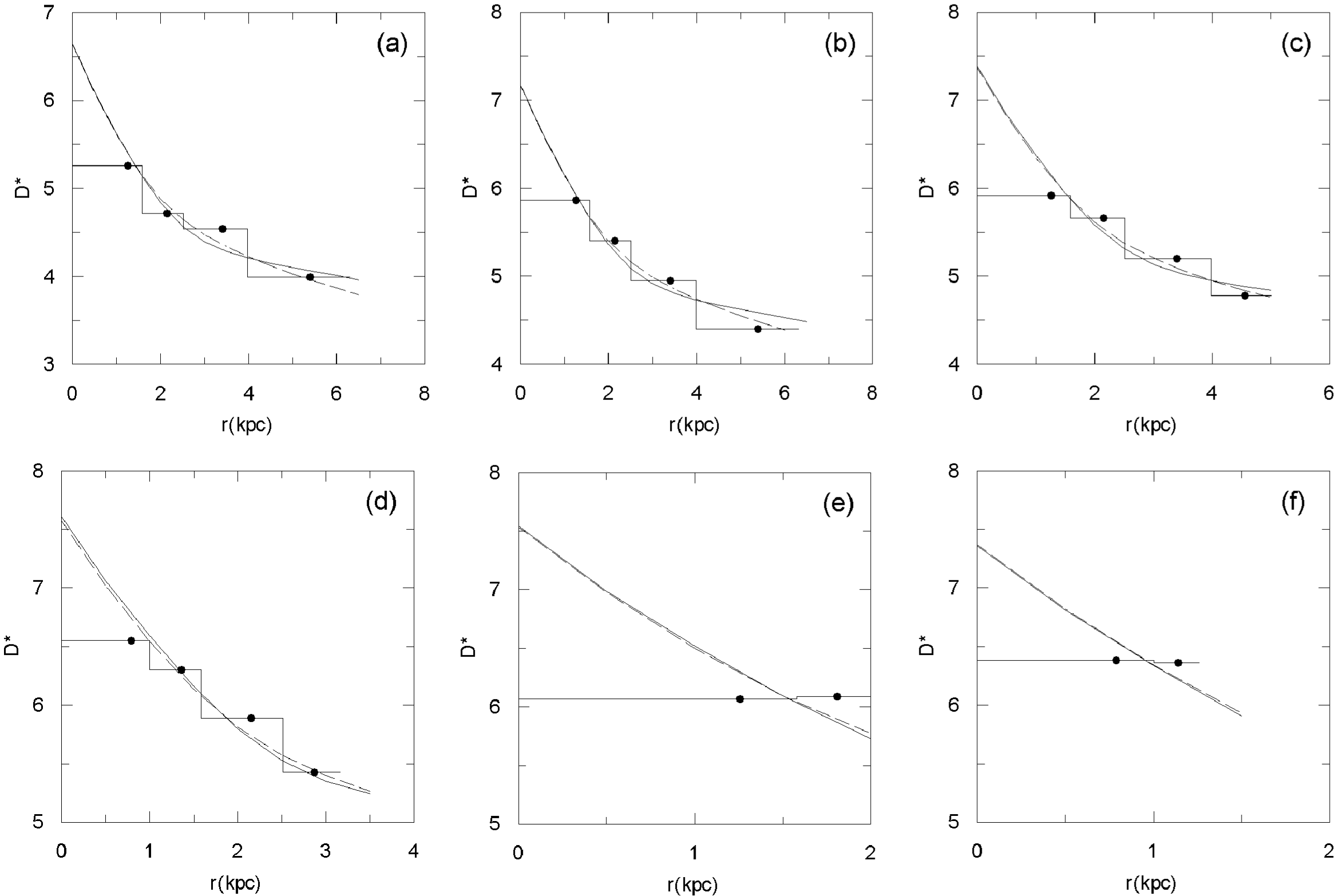
Figure 5: Logarithmic space-density histograms for all populations, within the limiting apparent magnitude of different $M(G)$ intervals: (a) $(2,3]$, (b) $(3,4]$, (c) $(4,5]$, (d) $(5,6]$, (e) $(6,7]$, and (f) $(7,8]$. ($\bullet$) centroid-distances within the limits of completeness for comparison with BRK (dashed curve) and GW (thin curve) model gradients.

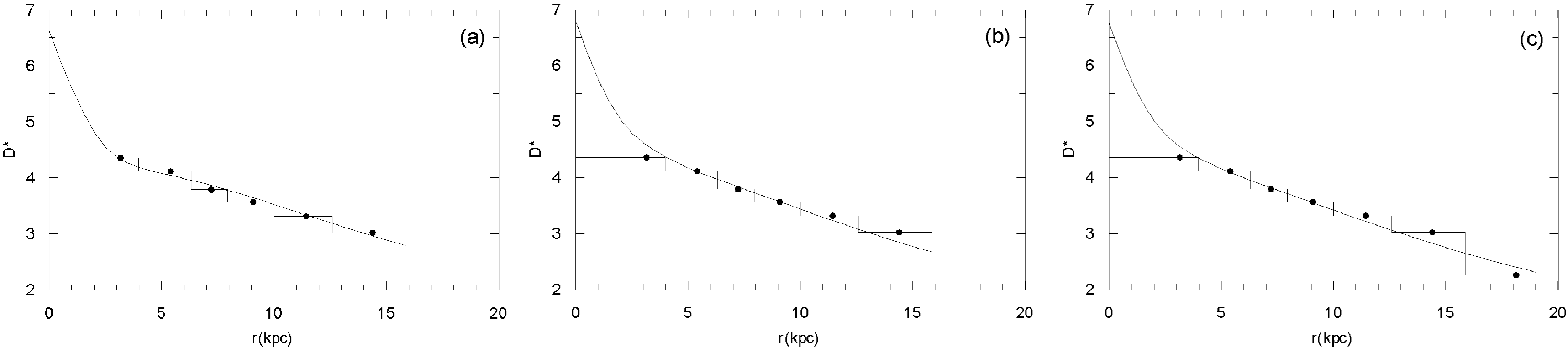
Figure 6: Logarithmic space-density histograms for giants for all populations ($M(G)\leq 2$ mag), within the limiting apparent magnitude. ($\bullet$) centroid-distance within the limiting distance of completeness for comparison with two model gradients, i.e. (a) GW, (b) BRK, and (c) BRK for a larger distance interval ($r\leq 19.95$ kpc).

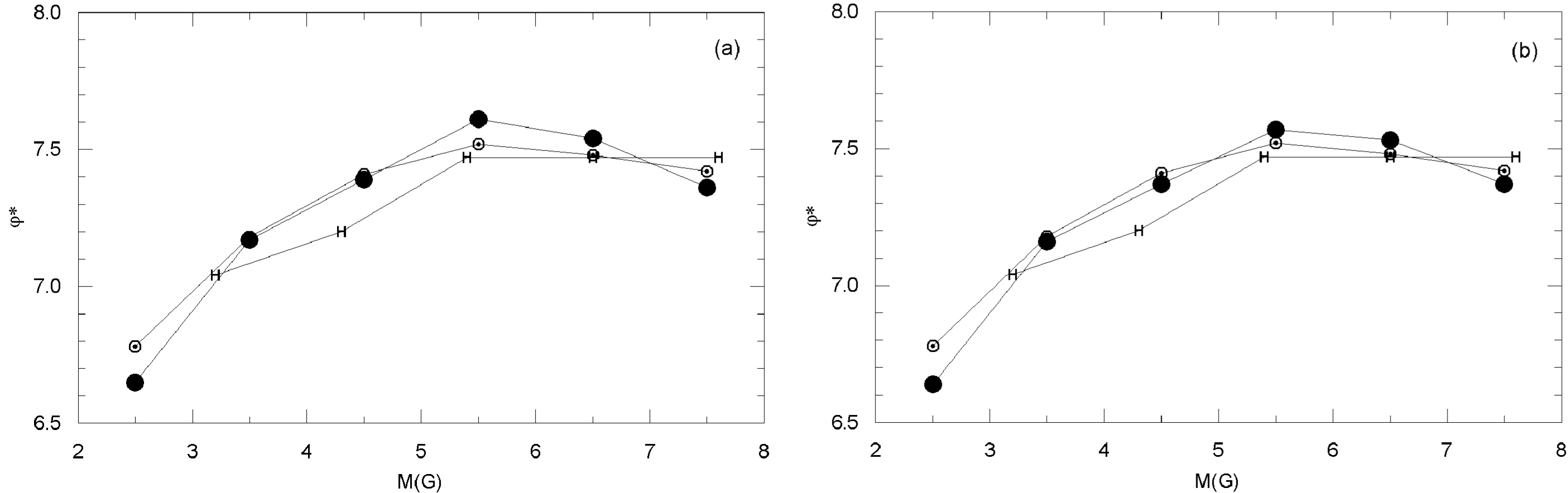
Figure 7: Logarithmic stellar luminosity function, implied by two model-gradients: (a) GW, and (b) BRK ($\bullet$) confronted to Gliese’s (1969) ($\odot$), and Hipparcos’ (JW 1997) (H) values.

5 Metallicity

The agreement of the observed space density functions with the model gradients, and of the local densities with Gliese’s (1969) and Hipparcos’ (JW 1997) values confirms both the separation of the stars into different luminosity classes and their absolute magnitude determination. Then, we can use this advantage to investigate the metallicity distribution and clarify the question of a probable metallicity gradient in the direction to our field. As cited in Section 3, the new formula for the metallicity determination for dwarfs is valid throughout the interval $-2.20\leq[Fe/H]\leq+0.20$ dex, hence metal-abundances $[Fe/H]\leq-2.20$ or $[Fe/H]>+0.20$ evaluated by the same formula are less certain. However, the number of stars with extreme metal abundances is not large, especially the metal-poor ones; thus, they do not affect our results significantly.

The metallicity distribution for dwarfs peaks at $[Fe/H]\sim 0.1$ dex, show a plateau between $[Fe/H]=-0.7$ and $-0.1$ dex, and decreases monotonously down to $[Fe/H]=-3$ dex (Fig.8a), however the metal-poor stars are small in number. Hence, the intermediate and metal rich stars dominate the distribution. Sub-giants, from the other hand, drawn from a larger spatial volume peak at a lower metallicity, i.e. $[Fe/H]=-0.6$ dex (Fig.8b).

The metallicities for all stars (dwarfs and sub-giants) summed over different $z$-distances show almost the same distribution, and hence a metallicity gradient can not be derived. On the other hand, dwarfs (only) with absolute magnitudes $4<M(G)\leq 6$, corresponding to spectral types F5-K0, which are long lived main-sequence stars, do show different metallicity distributions and reveal a metallicity gradient (Fig.9). Actually, the peaks for $[Fe/H]\cong-0.40$ and $\cong-0.80$ dex for the $z$-interval $0.75<z\leq 1.5$ kpc in Fig.9b (marked with numbers 1 and 2), shift to $[Fe/H]\cong-0.60$ and $[Fe/H]\cong-1.00$ dex, respectively, for the interval $1.5<z\leq 2.5$ kpc in Fig.9c (again, marked with numbers 1 and 2). Thus, for both displacements we get $d[Fe/H]/dz\cong-0.20$ dex/kpc. No any radial metallicity gradient could be detected for the same sample.

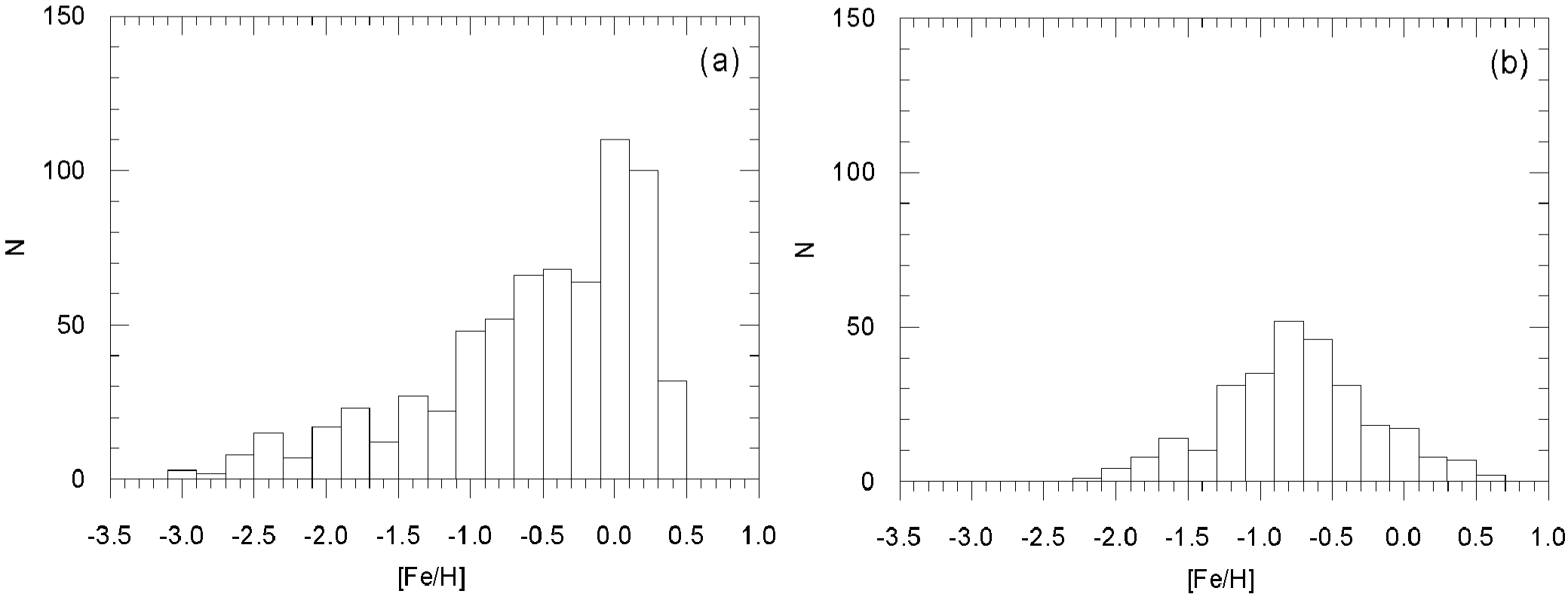
Figure 8: The metallicity distribution for dwarfs (a) and sub-giants (b).

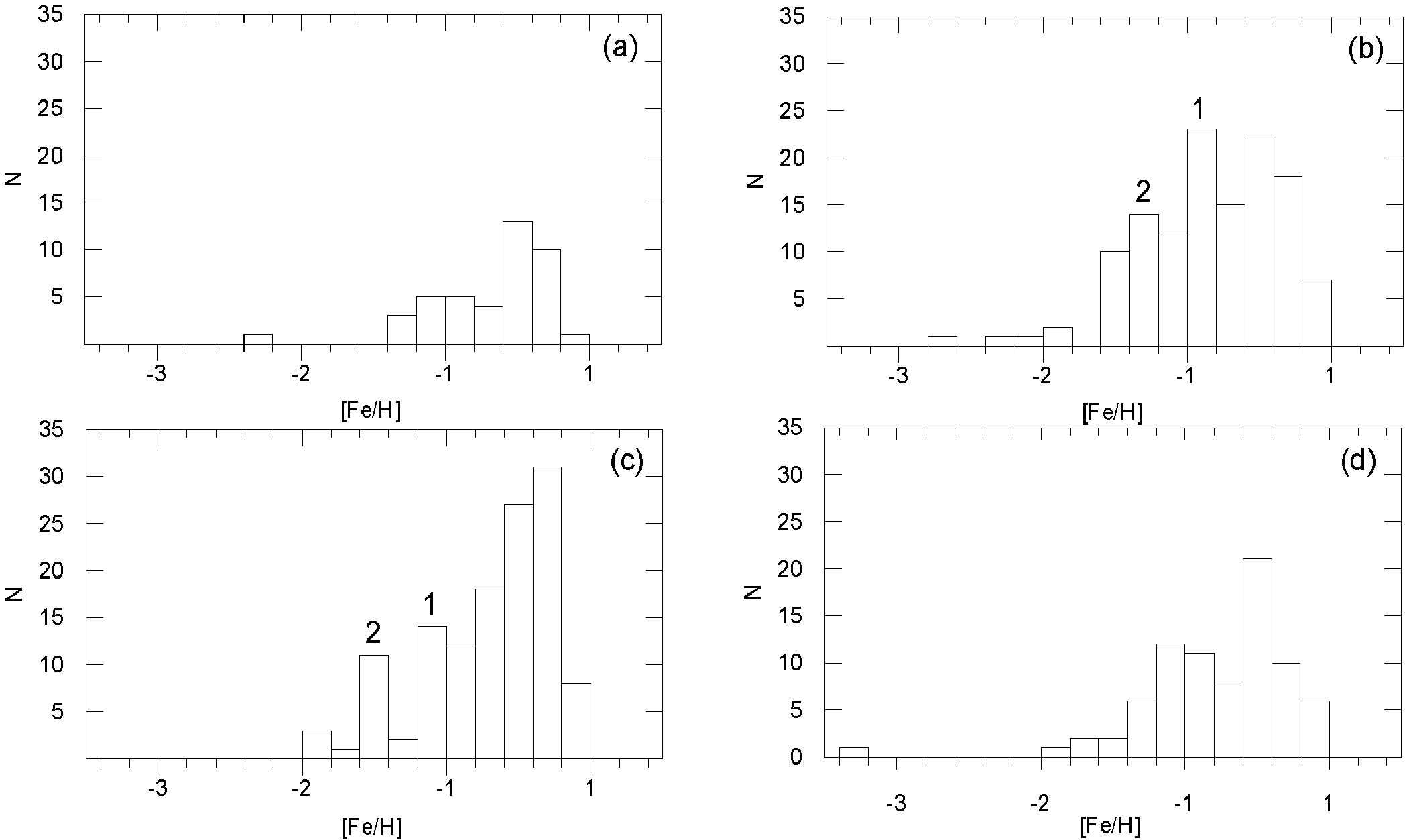
Figure 9: Metallicity distribution for dwarfs (only) with $4<M(G)\leq 6$ mag, corresponding to spectral types F5-K0, for four $z$-intervals: (a) $0<z\leq 0.75$, (b) $0.75<z\leq 1.5$, (c) $1.5<z\leq 2.5$, and (d) $2.5<z\leq 4$ kpc. The comparison of Fig.9b and 9c reveals a metallicity gradient of $d[Fe/H]/dz=-0.20$ dex/kpc.

Within the limiting distance of completeness (arrows, Fig.10) the spatial distribution for dwarfs and sub-giants shows that $z=1.6$ kpc and $z=2.75$ kpc are the borders of dominating regions of three populations, i.e. Population I (thin disk), Intermediate Population II (thick disk), and Extreme Population II (halo) (for separation of field stars into different population types see Karaali 1994). Hence, the metallicity gradient cited above covers both disks. The metallicity distribution for dwarfs and sub-giants with $1.6<z\leq 2.75$ kpc, i.e. for the thick disk, gives a bimodal distribution (Fig.11): the first mode, $[Fe/H]=-0.63$ dex, corresponds to the metal abundance assigned to the thick disk when it was introduced into the literature (Gilmore & Wyse 1985, Wyse & Gilmore 1986), and the second one, $[Fe/H]=+0.06$, to the metallicity which was cited for thick disk very recently (Carney 2000, Karaali et al. 2000). Although the number of super-solar metallicity stars seems to be larger than usually expected at distance $z=1.6$ kpc above the galactic plane, we accept this result regarding the procedures used for distance and metallicity evaluation. Actually, the luminosity functions implied by two model gradients cited above (Fig.7) show that our distance estimation is accurate, as well as the procedure of Carney (1979) (see Appendix) adopted for metallicity estimation.

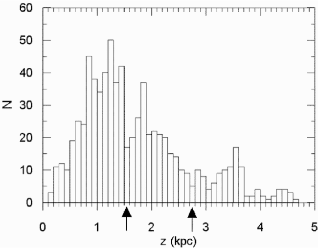
Figure 10: The spatial distribution for dwarfs and sub-giants within the limiting distance of completeness. The distances to the Galactic plane $z=1.6$ kpc and $z=2.75$ kpc (shown by arrows) are the borders of three populations, Population I (thin disk), Intermediate Population II (thick disk), and Extreme Population II (halo).

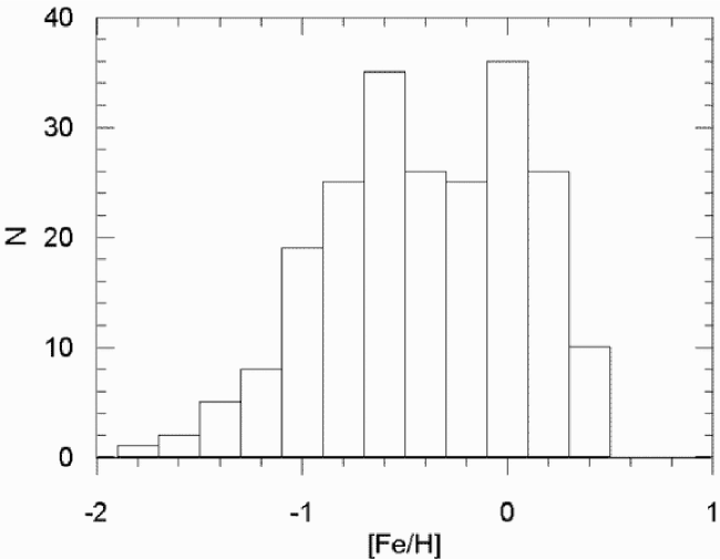
Figure 11: The metallicity distribution for dwarfs and sub-giants with $1.6<z\leq 2.75$ kpc, i.e. for the thick disk, giving a bimodal distribution. The first mode at $[Fe/H]=-0.63$ dex corresponds to the canonical metal abundance assigned to the thick disk (Gilmore & Wyse 1985, Wyse & Gilmore 1986, Buser et al. 1999, and Rong et al. 2001), and the second at $[Fe/H]=+0.06$ dex to the metallicity cited for the same component of the Galaxy very recently (Carney 2000, Karaali et al. 2000).

6 Summary and conclusion

The re-investigation of this field has been attractive because it provides illustrative and effective applications of a number of tools: the extra-galactic objects identified by comparison of Basel and Minnesota charts, and a small region with size 0.104 square-degrees contaminated by stars of the cluster M5 and affected by background light of bright star HD 136202 ($\alpha=15^{h}~{}19^{m}~{}18^{s}.80$, $\delta=+01^{o}~{}45{{}^{\prime}}~{}55{{}^{\prime\prime}}.5$, epoch 2000) are excluded from the program. Additionally, the evolved stars (sub-giants and giants) are separated from the dwarfs by an empirical method which has been used successfully in our recent works (Karaali 1992, Karaali et al. 1997, Ak et al. 1998, Karataş et al. 2001, Karaali et al. 2003), and the absolute magnitudes are determined by the colour-magnitude diagrams of Buser & Fenkart (1990), and Buser et al. (2000), obtained via synthetic photometry. Resulting logarithmic space densities agree with the model gradients of BRK, and GW. The luminosity function, which reflects the local densities, also agrees with the Gliese (1969) and Hipparcos (JW 1997) functions for the absolute magnitude intervals $2<M(G)\leq 3$, $3<M(G)\leq 4$, $4<M(G)\leq 5$, $5<M(G)\leq 6$, $6<M(G)\leq 7$, and $7<M(G)\leq 8$. However, for the giants two different local densities are in consideration, i.e. the comparison of observed space density histograms with the model gradients of GW give $D^{*}(0)=6.63$, rather close to that of Gliese (1969), and a slightly higher value, $D^{*}(0)=6.79$, when compared with BRK model gradients. From this we can conclude that the separation of field stars into different categories is probably carried out correctly.

The agreement cited above is used to advantage in treating the metallicity distribution for dwarfs and subgiants, and in looking for a probable metallicity gradient in this direction of the Galaxy. No different distribution can be observed for different $z$-distances from the Galactic plane, when dwarfs and sub-giants are considered together. However, this is not the case for dwarfs only, with absolute magnitudes $4<M(G)\leq 6$, corresponding to spectral types F5-K0, the long lived main-sequence stars. The difference between the two peaks in the metallicity distribution for $0.75<z\leq 1.5$ kpc and $1.5<z\leq 2.5$ kpc reveals a metallicity gradient $d[Fe/H]/dz\cong-0.20$ dex/kpc (Fig.9).

The metallicity for the thick disk ($1.6<z\leq 2.75$ kpc) shows a bimodal distribution (Fig.11): the first mode, $[Fe/H]=-0.63$ dex, represents the canonical metal abundance assigned to the thick disk (Gilmore & Wyse 1985, Wyse & Gilmore 1986, Buser et al. 1999, Rong et al. 2001, Karaali et al. 2003), and the second, $[Fe/H]=+0.06$ dex, corresponds to the value cited very recently (Carney 2000, Karaali et al. 2000). The metal-poor tail claimed by many authors (Rogers & Roberts 1993, Layden 1995, Beers & Sommer-Larsen 1995, Norris 1996, Chiba & Yoshii 1998, and Karaali et al. 2000) also exists in this direction.

This is one of the individual-field investigations of the Basel program, which offers space density functions in agreement with two Galactic model gradients, local space densities close to Gliese’s (1969) and Hipparcos’ (JW 1997) values, and vertical metallicity gradients which cover both the thin and thick disks. Thus, we confirm the works of Reid & Majewski (1993), Chiba & Yoshii (1998), Buser et al. (1999), Rong et al. (2001), and Karaali et al. (2003).

Appendix

We adopted the procedure used by Carney to obtain an equation for deriving the metallicity of a dwarf star from its observed ultra-violet excess, $\delta_{U-G}$. Two steps were followed for our purpose: in the first step, $UBV$ data for 52 and 24 dwarfs taken from Carney (1979) and Cayrel de Strobel et al. (1997), respectively, are transformed to the $RGU$ system by means of the metallicity-dependent conversion equations of Güngör-Ak (1995). The ($U-G$, $G-R$) main-sequence of the Hyades, transformed from $UBV$ to $RGU$ by the same formulae, is used as a standard sequence for ultra-violet excess evaluation. The transformation formulae just cited, or those of Buser (1978), may be used to show that the guillotine factors given by Sandage (1969) for $UBV$ photometry also apply for normalizing the ultra-violet excesses obtained on the $RGU$-photometric system, as follows: The equations which transform $U-B$ and $B-V$ colour indices of a star to the $G-R$ and $U-G$ colour indices are generally given by

$$G-R=a_{1}(U-B)+b_{1}(B-V)+c_{1},$$ (1)

$$U-G=a_{2}(U-B)+b_{2}(B-V)+c_{2},$$ (2)

where $a_{i}$, $b_{i}$, and $c_{i}$ (i = 1, 2) are parameters to be determined. Let us write equation (2) for two stars with the same $B-V$ (or equivalently $G-R$), i.e. for a Hyades star (H) and for a star (*) whose ultra-violet excess would be normalized,

$$(U-G)_{H}=a_{2}(U-B)_{H}+b_{2}(B-V)+c_{2},$$ (3)

$$(U-G)_{*}=a_{2}(U-B)_{*}+b_{2}(B-V)+c_{2}.$$ (4)

Then, the ultra-violet excess for the star in question, relative to the Hyades star is,

$$(U-G)_{H}-(U-G)_{*}=a_{2}[(U-B)_{H}-(U-B)_{*}]$$ (5)

or, in standard notation,

$$\delta(U-G)=a_{2}\delta(U-B).$$ (6)

Now, for another star with the same metal-abundance $[Fe/H]$ but with $B-V=0.60$ mag, (or its equivalent $G-R=1.08$) we get, in the same way,

$$\delta(U-G)_{1.08}=a_{2}\delta(U-B)_{0.60}.$$ (7)

Equations (6) and (7) give,

$$\frac{\delta(U-G)_{1.08}}{\delta(U-G)}=\frac{\delta(U-B)_{0.60}}{\delta(U-B)}=f,$$ (8)

where $f$ is the ultra-violet excess conversion (or guillotine) factor in question. Hence, the $RGU$-photometric $\delta(U-G)$ can be normalised by the same $f$ factors as are used in $UBV$ photometry.

In the second step, 76 stars are separated into 14 metallicity intervals, with different bin sizes, chosen such as to provide an almost equal number of stars in each bin. The least-squares method is used to obtain a calibration between the normalized ultra-violet excess $\delta_{1.08}$ and metallicity $[Fe/H]$. This binning provides equal-weight data for 14 points in Fig.12, which represent the mean metallicities and mean $\delta_{1.08}$ excesses for each bin. The constant term $a_{o}$ in the equation,

$$[Fe/H]=a_{o}+a_{1}\delta_{1.08}+a_{2}\delta^{2}_{1.08}$$ (9)

is assumed to be $a_{o}=0.11$ for consistency with the metallicity of the Hyades cited by Carney (1979). The least-squares method gives $a_{1}=-2.22$ and $a_{2}=-7.95$; thus,

$$[Fe/H]=0.11-2.22\delta_{1.08}-7.95\delta^{2}_{1.08}.$$ (10)

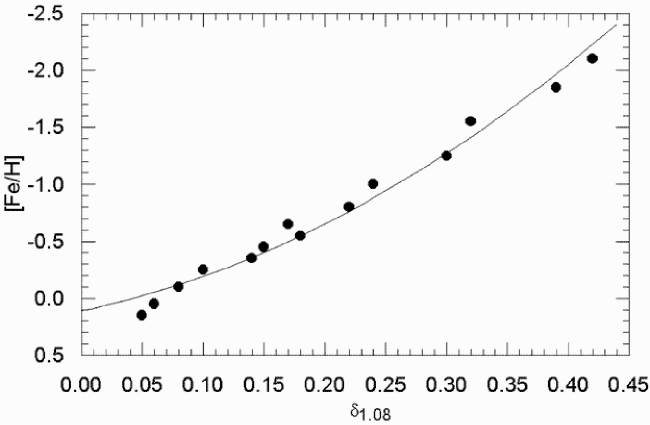
Figure 12: $[Fe/H]$ metallicity versus normalized $\delta_{1.08}$ ultra-violet excess for $RGU$ photometry.

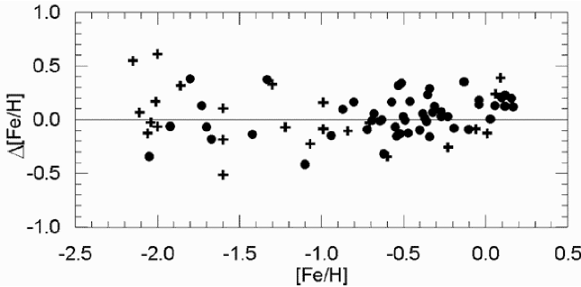
Figure 13: $\Delta[Fe/H]$ versus metallicity, where $\Delta[Fe/H]$ is the difference between the original metallicities and the evaluated ones, utilising the new calibration, $[Fe/H]=0.11-2.22\delta_{1.08}-7.95\delta^{2}_{1.08}$. Symbols: ($\bullet$) stars from Carney (1979), and (+) stars from Cayrel de Strobel et al. (1997).

The differences between the metallicities evaluated by means of equation (10) and the original ones, i.e. $\Delta[Fe/H]$, versus the original metallicities are given in Fig.13. The differences are large only for a few metal-poor stars, while the scatter relative to the line $\Delta[Fe/H]=0.0$ dex is small. Actually the mean of the differences (for all stars) is only 0.02 dex, while the probable error for the mean is small, $p.e.=\pm 0.15$ dex, indicating that the new calibration can be used with good accuracy.

Dwarfs used for the new metallicity calibration are identified either according to their spectral types or surface gravities.

References

Ak, S. G., Karaali, S., & Buser, R. 1998, A&AS, 131, 345

Becker, W., Steinlin, U., & Wiedeman, D. 1978, Photometric catalogue for stars in selected areas and other fields in the $RGU$-system (V). Basel; Astronomical Institute of the University of Basel

Beers, T. C., & Sommer-Larsen, J. 1995, ApJS, 96, 175

Bilir, S., Karataş, Y., & Ak, S. G. 2003, TJPh, 27, 235

Buser, R. 1978, A&A, 62, 425

Buser, R., & Fenkart, R. P. 1990, A&A, 239, 243

Buser, R., & Rong, J. 1995, BaltA, 4, 1

Buser, R., Rong, J., & Karaali, S. 1998, A&A, 331, 934 (BRK)

Buser, R., Rong, J., & Karaali, S. 1999, A&A, 348, 98

Buser, R., Karataş, Y., Lejeune, Th., Rong, J. X., Westera, P., & Ak, S. G. 2000, A&A, 357, 988

Carney, B. W. 1979, ApJ, 233, 211

Carney, B. W. 2000, Proceedings of the $35^{th}$ Liége Int. Astrophys. Coll., July 5-8, 1999, p. 287

Cayrel de Strobel, G., Soubiran, C., Friel, E. D., Ralite, N., & Francois, P. 1997, A&AS, 124, 299

Chiba, M., & Yoshii, Y. 1998, AJ, 115, 168

Del Rio, G., & Fenkart, R. P. 1987, A&AS, 68, 397

Fenkart, R. P., & Karaali, S. 1987, A&AS, 69, 33

Fenkart, R. P., & Karaali, S. 1990, A&AS, 83, 481

Gilmore, G., & Wyse, R. F. G. 1985, AJ, 90, 2015 (GW)

Gliese, W. 1969, Ver ff. Astron. Rechen Inst. Heidelberg No:22

Güngör-Ak, S. 1995, Ph. D. Thesis, Istanbul Univ.

Jahreiss, H., & Wielen, R. 1997, in: HIPPARCOS’97. Presentation of the HIPPARCOS and TYCHO catalogues and first astrophysical results of the ipparcos space astrometry mission., Battrick, B., Perryman, M. A. C., & ernacca, P. L., (eds.), ESA SP-402, Noordwÿk, p.675 (JW)

Karaali, S. 1992, VIII. Nat. Astron. Symp. Eds. Z. Aslan and O. Gölbaşı, Ankara - Turkey, p.202

Karaali, S. 1994, A&AS, 106, 107

Karaali, S., Karataş, Y., Bilir, S., & Ak, S. G. 1997, IAU Abstract Book, Kyoto, p.299

Karaali, S., Karataş, Y., Bilir, S., Ak, S. G., & Gilmore, G. F. 2000, The Galactic Halo: from Globular Clusters to Field Stars. $35^{th}$ Liége Intr. Astr. Coll. Edts. A. Noel et al., p. 353

Karaali, S., & Bilir, S. 2002, TJPh, 26, 427

Karaali, S., Ak, S. G., Bilir, S., Karataş, Y. & Gilmore, G. 2003, MNRAS, 343, 1013

Karataş, Y., Karaali, S., & Buser, R. 2001, A&A, 373, 895

Layden, A. C. 1995, AJ, 110, 2288

Norris, J. E. 1996, ASP Conf. Ser. Vol.92, p.14, Eds. H. L. Morrison & A. Sarajedini

Reid, N., & Majewski, S. R. 1993, ApJ, 409, 635

Rodgers, A. W., & Roberts, W. H. 1993, AJ, 106, 1839

Rong, J., Buser, R., & Karaali, S. 2001, A&A, 365, 431

Sandage, A. R. 1969, ApJ, 158, 1115

Schlegel, D. J., Finkbeiner, D. P., & Davis, M. 1998, ApJ, 500, 525

Wyse, R. F. G., Gilmore, G. 1986, AJ, 91, 855