Magnetized cosmic walls

Nonlinear growth of one-dimensional density structures with a frozen-in magnetic field is investigated in Newtonian cosmology. A mechanism of magnetic field amplification is discussed. We discuss the relation between the initial conditions for the velocity field and the basic time-scales determining the growth of the magnetized structure.

1 Introduction

During the last decade the evidence large-scale cosmological magnetic fields has systematically grown. Fields of several microgauss have been measured beyond the galaxy clusters (Kim et al. 1991); the Rotation Measure (Kronberg 1994) confirms the existence of coherent magnetic field on Mpc scales or larger. The recent discovery of large-scale diffuse radio emission testifies to the presence of magnetic fields of $\sim 0.1\leavevmode\nobreak\ \mu$G, along the 6 Mpc filament (Bagchi et al. 2002), with evidence for their coherent nature.

Understanding of the magnetic field behaviour at different phases of the matter-dominated era is crucial to explain the microgauss fields observed in high redshift objects $z\geq 2$; starting from the damped Ly $\alpha$ systems, through the distant radiogalaxies and the galaxy clusters up to the scales typical of galaxy superclusters. While the magnetic field of galaxies may result from dynamo effects, the fields at larger scales cannot be explained by the same mechanism. Here there is either no rotation, necessary for dynamo action, or the structures are dynamically too young to leave dynamo action enough time to operate. Magnetic fields at Mpc scales are likely to be primordial. Some pre-dynamo mechanisms of the primeval magnetic field amplification must be at work at least in the linear and weakly nonlinear regime.

In this paper we discuss the mutual relationships between density growth and the magnetic field evolution in early nonlinear stages, when the wall or filamentary structure is formed. We investigate whether the growing planar density structure may drag and amplify the magnetic field. We employ the exact solutions for 2-D (pancake ) inhomogeneity evolution in the Newtonian description and emphasize the role of initial conditions, in particular, the large-scale primordial flows. The magnitude of primordial velocity fields at recombination determines the time and the growth rate of density fluctuation. As a consequence, it defines the duration time of the pre-dynamo and dynamo amplification phase. To avoid problems with a mathematical definition of the weakly nonlinear regime we work with fully nonlinear equations and their solutions. Although finally we refer to the regime where the density contrast ${\Delta}$ is between $1$ and $100$ (which is relevant for the cosmological structures we discuss), dynamical equations are true for ${\Delta}>100$.

Magnetohydrodynamic equations in the covariant notation are given in Section 2. Simplifying physically relevant assumptions and the resulting nonlinear perturbation equations are discussed in Section 3. Nonlinear solutions for the density contrast and the magnetic field enhancement are given in Section 4. Section 5 contains numerical estimations and graphical presentation of the magnetized pancake formation.

2 Magnetized self-gravitating fluid

Magnetohydrodynamic equations for self-gravitating fluid with infinite conductivity (Chandrasekhar $\&$ Fermi 1953, Wasserman 1978, Papadopulos $\&$ Esposito 1982), expressed in a manifestly covariant way, form a dynamical system for the density ${\rho}$, the expansion rate $\vartheta$, and the magnetic field $H^{i}$

$$\dot{{\rho}} = -{\rho}\vartheta$$ (1)

$$\dot{\vartheta} = -{1\over 3}\vartheta^{2}-{4\pi}\kappa{\rho}-2\sigma^{2}+2\omega^{2}+{\left({1\over{\rho}}(H^{i}H_{j}-{1\over 2}H^{2}\delta^{i}_{j})^{;j}-{1\over{\rho}}p^{;i}\right)_{;i}}$$ (2)

$$\dot{H^{i}} = \sigma^{i}_{j}H^{j}+\omega^{i}_{j}H^{j}-{2\over 3}\vartheta H^{i}$$ (3)

Hydrodynamic scalars $\sigma$ and $\omega$, which measure the shear and the rotation, respectively,

$$\sigma = {1\over 2}(\sigma_{ik}\sigma^{ik})^{1/2},\leavevmode\nobreak\ \leavevmode\nobreak\ \leavevmode\nobreak\ \leavevmode\nobreak\ \leavevmode\nobreak\ \leavevmode\nobreak\ \sigma_{ik}={1\over 2}(v_{i;k}+v_{k;i}-{2\over 3}\delta_{ik}v^{j}_{;j}),$$ (4)

$$\omega = {1\over 2}(\omega_{ik}\omega^{ik})^{1/2},\leavevmode\nobreak\ \leavevmode\nobreak\ \leavevmode\nobreak\ \leavevmode\nobreak\ \leavevmode\nobreak\ \leavevmode\nobreak\ \omega_{ik}={1\over 2}(v_{i;k}-v_{k;i}).$$ (5)

$v^{i}$ stands for the fluid velocity, its divergence builds the expansion rate $\vartheta=v^{i}_{;i}$. Semicolon means the covariant derivative with respect to the space coordinates, dot stands for the time convective derivative, e.g. $\dot{{\rho}}={\partial{\rho}/\partial t+v^{i}{\rho}_{;i}}$, while $\delta^{ij}$ is the Kronecker delta; the Einstein summation convention is employed. Equations (1-3) are coordinate-independent. (In the Cartesian coordinates, covariant derivatives reduce to the partial derivatives, and tensor indices are raised and lowered by Kronecker delta). Equation (1) is the continuity equation. Equation (2) is a Newtonian analogue of the Raychaudhuri-Ehlers equation (Ellis 1971) — a scalar form of the equation of motion for continuously gravitating media with the Poisson equation included. System (1-3) has the same form in general relativity and Newtonian theory (Ellis 1971, compare also Tsagas $\&$ Barrow 1997), and therefore is of particular interest in the cosmological context.

The approximation of infinite conductivity results in a vanishing electric field. The magnetic contribution to the equation of motion is quadratic in $H^{i}$ (the last term in eq. (2)), and therefore, can be neglected in the weak magnetic field limit. In this limit the system (1-3) splits into the autonomous system (1-2) and the induction equation (3). Then, the fluid dynamics is entirely determined by gravitational forces, while the magnetic field is dragged along by fluid flow.

3 Planar symmetry

Below we consider a model based on the following assumptions:

1. The unperturbed “background space” is an isotropic and homogeneous (Newtonian) universe.

2. The initial perturbation state is given at random, i.e. perturbation in the density and velocity fields ${\Delta}_{(ini)}=\left[{\delta\rho\over\rho{{}_{(0)}}}\right]_{(ini)}$ and ${\Theta}_{(ini)}=\left[{\delta\vartheta\over\vartheta{{}_{(0)}}}\right]_{(ini)}$ are independent quantities. The perturbation is initially small, i.e. ${\Delta}_{(ini)}\ll 1$ and ${\Theta}_{(ini)}\ll 1$

3. After the recombination epoch, the infinite conductivity approximation is adequate. The electric field vanishes ($E^{i}\simeq 0$), while the magnetic field $H^{i}$ is frozen (Chandrasekhar $\&$ Fermi 1953). The matter pressure is negligible ($p=0$)

4. During the considered period the primordial magnetic fields and their gradients are small compared with the density and the density gradients, respectively ($H_{i}H^{i}\ll{\rho}$, $H_{i;j}H^{i}\ll{\rho}_{;j}$). In the noncovariant approach to MHD this implies a small value of the ratio of Lorentz force $F_{L}$ to the gravitational force $F_{G}$.

5. The perturbation is rotationless and has a planar symmetry, i.e. the velocity potential ${V}(t,x^{i})$ can be expressed as ${V}(t,x^{i})={V}_{0}(t,x^{i})+{\delta V}(t,x^{3})$, where ${V}_{0}(t,x^{i})={1\over 6}\vartheta{{}_{(0)}}x_{k}x^{k}$ stands for unperturbed Hubble flow, and the perturbation ${\delta V}(t,x^{3})$ is independent of two of Cartesian coordinates. Consequently, all the hydrodynamic scalars depend solely on time and on the only one space variable $x^{3}\equiv z$ , the one parallel to the fluid contraction (orthogonal to the pancake plane).

Under these assumptions the system (1)-(3) can be divided into the background dynamics

$$\dot{{\rho}}{{}_{(0)}} = {\rho}{{}_{(0)}}\vartheta{{}_{(0)}}$$ (6)

$$\dot{\vartheta}{{}_{(0)}} = -{1\over 3}\vartheta{{}_{(0)}}^{2}-{4\pi}\kappa{\rho}{{}_{(0)}}\ ,$$ (7)

where the “unperturbed” magnetic field is obviously absent, and the propagation equations for inhomegeneities

$$\dot{\delta{\rho}} = -\vartheta{{}_{(0)}}\delta{\rho}-{\rho}{{}_{(0)}}\delta\vartheta-\delta{\rho}\delta\vartheta$$ (8)

$$\dot{\delta\vartheta} = -{4\pi}\kappa\delta{\rho}-{2\over 3}\vartheta{{}_{(0)}}\delta\vartheta-\delta\vartheta^{2}$$ (9)

$$\dot{H}^{i} = \delta\vartheta(\delta_{{\it 3}}^{i}\delta^{{\it 3}}_{j}-\delta_{j}^{i})H^{j}-{2\over 3}\vartheta{{}_{(0)}}H^{i}\ .$$ (10)

The perturbations $\delta{\rho}={\rho}-{\rho}{{}_{(0)}}$ and $\delta\vartheta=\vartheta-\vartheta{{}_{(0)}}$ are defined as differences between local and background values. They are not assumed to be small, hence nonlinear terms in (8-9) remain. The shear tensor for planar perturbation

$$\sigma_{ik}={\sigma\over\sqrt{3}}(3\delta_{i}^{\it 3}\delta_{k}^{\it 3}-\delta_{ik})={\delta\vartheta\over{3}}(3\delta_{i}^{\it 3}\delta_{k}^{\it 3}-\delta_{ik})$$ (11)

has been employed to derive equations (9 and 10). In particular the shear scalar $\sigma$ has been expressed by the variation in the expansion rate $\delta\vartheta$, i.e. ${\sigma}={1\over\sqrt{3}}\delta\vartheta$. The autonomous sub-system (8-9) can be evaluated to a single second order differential equation for the density contrast ${\Delta}={\delta\rho\over\rho{{}_{(0)}}}$

$$\left({\Delta}\right)^{..}-{2\over(1+{\Delta})}\left(\dot{{\Delta}}\right)^{2}=-{2\over 3}\vartheta{{}_{(0)}}\dot{{\Delta}}+4\pi\kappa{\rho}{{}_{(0)}}{\Delta}\left(1+{\Delta}\right)$$ (12)

and solved independently.

4 The evolution of planar structures

Equation (12) reduces to the Jeans-Bonnor equation (Bonnor 1957, Weinberg 1972)

$$\left({\mu}\right)^{..}=-{2\over 3}\vartheta{{}_{(0)}}\dot{{\mu}}+4\pi\kappa{\rho}{{}_{(0)}}{\mu}$$ (13)

under the change of the perturbation variable (compare Buchert 1989 in the context of the Zeldovich approximation)

$${\mu}={{\Delta}\left(1+{\Delta}\right)^{-1}}\ .$$ (14)

This enables one to express the finite amplitude (nonlinear) perturbations as functions of the solutions to the linear equation (13). Equation (13) rewritten in the conformal time $\eta=\int a(t)^{-1}dt$ takes the form

$${\mu}^{\prime\prime}+{a^{\prime}\over a}{\mu}^{\prime}-{3\over 2}\left[K+\left({a^{\prime}\over a}\right)^{2}\right]=0\ ,$$ (15)

where the dimensionless scale factor $a(\eta)$, formally defined by the differential equation $\vartheta_{0}(\eta)^{\prime}=3{a(\eta)^{\prime}\over a(\eta)^{2}}$, satisfies the Friedman equation for a dust-filled universe

$${K\over a^{2}}-{a^{\prime}\over a^{2}}+2{a^{\prime\prime}\over a^{3}}=0$$ (16)

and can be found in the exact form

$$a(\eta)={{{M}}\over{3K}}\sin^{2}\left(\sqrt{K}\eta\over 2\right)\ .$$ (17)

Prime in (15), (16) and all the equations below is the differentiation with respect to $\eta$, both $K$ and ${M}=a^{3}(\eta){\rho}$ are constants of motion. The two independent solutions of the equation (15) read

$${\mu}_{1}(\eta) = -10{{M}\over K}\left[1+{3\over 2}\left(-2+\sqrt{K}\eta\cot{\sqrt{K}\eta\over 2}\right)\sin^{-2}{\sqrt{K}\eta\over 2}\right]$$ (18)

$${\mu}_{2}(\eta) = \left({{M}\over K}\right)^{-3/2}\left[1+\tan^{-2}{\sqrt{K}\eta\over 2}\right]\cot^{3}{\sqrt{K}\eta\over 2}$$ (19)

and in the $K\rightarrow 0$ limit yield ${\mu}_{1}(\eta)={M}\eta^{2}$ and ${\mu}_{2}(\eta)={M}^{-3/2}\eta^{-3}$, respectively. The arbitrary solution to (13) is a linear combination

$${\mu}(\eta)=c_{1}{\mu}_{1}(\eta)+c_{2}{\mu}_{2}(\eta)\ ,$$ (20)

while the original perturbation ${\Delta}$ can be found by use of the reciprocal transform

$${\Delta}(\eta)={{\mu}(\eta)\over{1-{\mu}(\eta)}}\ .$$ (21)

Although the solutions ${\mu}(\eta)$ form the linear space (20), the solutions $\Delta(\eta)$ to equation (12) obviously do not. On the other hand the time evolution of the magnetic field is governed by the linear equation (10), which after investing (8) can be integrated exactly. The solution written covariantly reads

$$H^{i}(\eta)={a^{2}_{{(ini)}}\over{a^{2}(1-{\mu}(\eta))}}(\delta_{j}^{i}-{\mu}(\eta)\delta_{{\it 3}}^{i}\delta^{{\it 3}}_{j})H^{j}_{{(ini)}}$$ (22)

and can also be expressed as a function of the density contrast ${\Delta}({\rm z})$ of the pancake structure observed at the redshift ${\rm z}$ (we write it in the matrix form)

$$\left(\begin{array}[]{c}H_{x}({\rm z})\\ H_{y}({\rm z})\\ H_{z}({\rm z})\end{array}\right)=\left({{\rm z}+1\over{\rm z}_{(ini)}+1}\right)^{2}\left(\begin{array}[]{ccc}{1+{\Delta}({\rm z})}&0&0\\ 0&{1+{\Delta}({\rm z})}&0\\ 0&0&1\\ \end{array}\right)\left(\begin{array}[]{c}H_{x}\\ H_{y}\\ H_{z}\end{array}\right)_{{(ini)}}\ .$$ (23)

Derivation of the formula (22-23) does not involve the Raychaudhuri equation. Therefore, (22-23) is well satisfied for arbitrary large magnetic fields, and is independent of the $p=0$ approximation. It expresses the amplification of the magnetic field during the one-dimensional fluid compression in a homogeneously expanding medium. It shows that the orthogonal component $H_{z}$ is systematically diluted during the universe expansion, while components parallel to the pancake plane increase with the local density. As a consequence, the relic magnetic field in a large-scale planar structure is amplified and flattened to the plane.

All the dynamical effects of gravity, pressure or magnetic field cumulate in the ${\mu}(\eta)$ or ${\Delta}({\rm z})$ evolution. For the dust filled universe in the weak magnetic field approximation the formulae (23), (20), (18), (19) and (17) constitute a closed form solution for the magnetic field enhancement.

5 Numerical estimations

It is reasonable to view the numerical results in the $K=0$ universe, where the linear solution for ${\mu}({\rm z})$ expressed as a function of the redshift ${\rm z}$ takes the form

$${\mu}({\rm z})={{\Delta}_{(ini)}\over 5}\left[3{\left(\sqrt{\frac{1+{\rm z}_{(ini)}}{1+{\rm z}}}\right)}^{2}+2{\left(\sqrt{\frac{1+{\rm z}_{(ini)}}{1+{\rm z}}}\right)}^{-3}\right]+{{\Theta}_{(ini)}\over 5}\left[{\left(\sqrt{\frac{1+{\rm z}_{(ini)}}{1+{\rm z}}}\right)}^{2}-{\left(\sqrt{\frac{1+{\rm z}_{(ini)}}{1+{\rm z}}}\right)}^{-3}\right]\ .$$ (24)

Consequently the perturbations ${\Delta}=\left[{\delta\rho\over\rho{{}_{(0)}}}\right]$, ${\Theta}=\left[{\delta\vartheta\over\vartheta{{}_{(0)}}}\right]$ and the magnetic field $H({\rm z})$ read respectively

$${\Delta}({\rm z}) = \frac{2({\Delta}_{(ini)}+3{\Theta}_{(ini)})+3({\Delta}_{(ini)}-2{\Theta}_{(ini)}){\left(\sqrt{\frac{1+{\rm z}_{(ini)}}{1+{\rm z}}}\right)}^{5}}{5{\left(\sqrt{\frac{1+{\rm z}_{(ini)}}{1+{\rm z}}}\right)}^{3}-2({\Delta}_{(ini)}+3{\Theta}_{(ini)})-3({\Delta}_{(ini)}-2{\Theta}_{(ini)}){\left(\sqrt{\frac{1+{\rm z}_{(ini)}}{1+{\rm z}}}\right)}^{5}}$$ (25)

$${\Theta}({\rm z}) = \frac{({\Delta}_{(ini)}+3{\Theta}_{(ini)})-({\Delta}_{(ini)}-2{\Theta}_{(ini)}){\left(\sqrt{\frac{1+{\rm z}_{(ini)}}{1+{\rm z}}}\right)}^{5}}{5{\left(\sqrt{\frac{1+{\rm z}_{(ini)}}{1+{\rm z}}}\right)}^{3}-2({\Delta}_{(ini)}+3{\Theta}_{(ini)})-3({\Delta}_{(ini)}-2{\Theta}_{(ini)}){\left(\sqrt{\frac{1+{\rm z}_{(ini)}}{1+{\rm z}}}\right)}^{5}}$$ (26)

$$H({\rm z}) = \left({{\rm z}+1\over{\rm z}_{(ini)}+1}\right)^{2}(1+{\Delta}({\rm z}))H_{(ini)}\ .$$ (27)

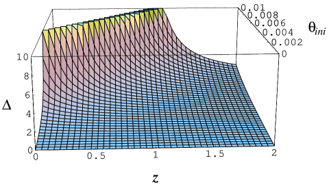
Formulae (25-27) show how the structure formation process depends on the initial conditions at the recombination, i.e. on the initial density fluctuation ${\Delta}_{(ini)}$ and the initial flow ${\Theta}_{(ini)}$ (the velocity divergence). Setting ${\Delta}_{(ini)}=10^{-6}$ at ${\rm z}=1200$, as suggested by the CMBR measurements, we draw ${\Delta}$ and ${\Theta}$ as functions of ${\rm z}$ and the initial flow ${\Theta}_{(ini)}$ (see Fig. 1 and Fig. 2).

Figure 1: Density contrast as a function of redshift $z$ and initial velocity flow ${\Theta}_{(ini)}$.

Figure 2: Velocity field contrast as a function of redshift $z$ and initial velocity flow ${\Theta}_{(ini)}$.

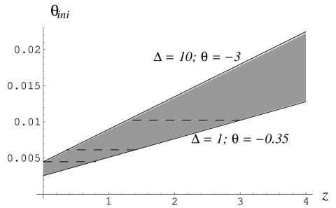
Galactic superclusters with the density contrast ${\Delta}\leq 100$ are considered as nonvirialized structures (Peacock 1999). Their length scales of about $\sim 10$ Mpc are typically expected at the moment of transition from the linear to nonlinear regime. The evolution of these structures relative to the initial values of the large scale inflows ${\Theta}_{(ini)}$ is presented in Fig 3. The evolutionary paths with different ${\Theta}_{(ini)}$ form horizontal lines, while the solid sloped lines mark the beginning (${\Delta}=1$, ${\Theta}=-0.35$) and the end (${\Delta}=10$, ${\Theta}=-3$) of the weakly nonlinear regime (the shaded region). The magnitudes of the contrasts at both characteristic moments are set to be compatible with the values obtained from the numerical simulation (Gramann et al. 2002). The region below the shaded region represents the linear evolution, while the region above — the strongly nonlinear collapse. The existence of the low ${\rm z}$ structures with ${\Delta}\leq 100$, confirmed by the observations, when compared with the theoretical low redshift behaviour (Fig 3) favours the initial inflow ${\Theta}_{(ini)}\simeq 10^{-3}$ at the recombination epoch.

Figure 3: Schematic diagram of weakly nonlinear evolution of the density and velocity contrasts. For both contrasts the ${\Delta}=const$ and ${\Theta}=const$ sections are presented. The solid lines correspond to the initial and final states of the previrial nonlinear evolution of ${\Delta}$ and ${\Theta}$. The shaded area represents all the evolutionary states between (${\Delta}=1$, ${\Theta}=-0.35$) and (${\Delta}=10$, ${\Theta}=-3$). Horizontal dashed lines show the evolutionary tracks.

The initial velocity field determines the basic time scales for the weakly and strongly nonlinear structure formation respectively, and consequently, defines the time scales for compression and magnification of the seed magnetic field. In particular, the time of entering the strongly nonlinear regime (${\Delta}\approx 150$) is crucial for the efficiency of the dynamo action (e.g. Widrow 2002). The amplification degree in this process exponentially depends on the time available for the dynamo mechanism to operate. The pre-dynamo magnetic field compression (Lesch et al. 1995) is followed by the dynamo amplification, which in the case of protogalaxies results in some $10^{4}-10^{10}$ enhancement in amplitude, depending on the time when the field reaches the observed value. The question if the dynamo mechanism is applicable to galactic cluster structures is still open. Even more intriguing is the origin of the almost equipartized supercluster magnetic fields ($\simeq 10^{-7}$) (Sigl et al. 1998). Fig. 3 illustrates that structures with initial inflow ${\Theta}_{(ini)}\simeq 10^{-2}$ reaches the weakly nonlinear regime (${\Delta}\simeq 1$) at redshift ${\rm z}=3$, and leaves the weakly nonlinear phase (${\Delta}\simeq 100$) at ${\rm z}=1.3$. A dynamo may operate then for $\simeq 8\times 10^{9}yr$, which (taking into account the typical dynamo time scale $\simeq 10^{9}yr$) results in the $\simeq 2\,10^{3}$ enhancement of magnetic field. On the other hand, for the structures with the initial inflows at the level of ${\Theta}_{(ini)}\approx 6\times 10^{-3}$ (or ${\Theta}_{(ini)}\approx 5\times 10^{-3}$), the beginning and the end of the previrial nonlinear stage occur at ${\rm z}\approx 1.4$ (z $\approx 0.8$) and ${\rm z}\approx 0.4$ (${\rm z}\approx 0$), respectively, which limits the dynamo operation phase to less than $2.3\times 10^{9}yr$ (or none). In this latter case i.e. for systems which presently attain the previrial collapse state (${\Delta}\simeq 100$ at $z\simeq 0$), the primordial magnetic field constrained at $z=10^{3}$ to magnitudes below $\sim 10^{-9}$ G (Barrow et al. 1997) are pre-dynamo amplified by merely 2 orders of magnitude.

6 Summary

We provided the nonlinear exact solutions for the density, velocity and magnetic fields for the pancake -type structures in the Newtonian expanding universe. The approximations of the potential velocity field and vanishing matter pressure have been employed. The time when the compressing flat structure enters the regime of nonlinear growth is controlled by the initial value of velocity field at the recombination. The structures accompanied by large hydrodynamic flows collapse earlier, i.e. the moment when dynamo mechanism may switch on occurs at higher redshifts, which eventually results in stronger magnetic field enhancement. For presently observed velocity fields, $10^{-1}$, (see, e.g. Dekel 1997) in supergalactic structures of $100$ Mpc and ${\Delta}\sim 1$ the initial inflows ${\Theta}_{(ini)}\simeq 10^{-3}$ and initial magnetic fields $H_{(ini)}\simeq 10^{-9}-10^{-8}$ Gauss are expected. The result is compatible with the simulation estimations (Gramann et al., 2002).

Firm evidence of primordial magnetic fields in structures at pre-virial stages is of particular importance, as these fields ”remember” the initial conditions and thus set constraints on the seed magnetic fields, density and velocity fields at the recombination. The observational techniques become more important (Faraday rotation measurements and the indications coming from the propagation of cosmic radiation UHE in the Local Supercluster), which potentially might distinguish between the large scale magnetic seed component from other magnetic fields of astrophysical origin (i.e. resulting from galactic dynamo, outflows from radiogalaxies etc.). The rotation measure which have the same sign along the Supercluster plane would suggest a coherent, relic field at this scale.

7 Acknowledgments

We thank the Referee for efforts to improve the manuscript.

References

Bagchi, J.,Ensslin, T., Miniati, F., et al. 2002, New Astron., 7, 249
Barrow, J., Ferreira, P., $\&$ Silk, J. 1997, Phys. Rev. Lett., 78, 3610
Bonnor, W. 1957, MNRAS, 117, 104
Buchert, T. 1989, A$\&$A, 223, 9
Chandrasekhar, S., $\&$ Fermi, E. 1953, ApJ, 118, 116
Dekel, A. 1997, in Formation of Structure in the Universe, ed. A. Dekel, J. Ostriker (Cambridge Univ. Press)
Ellis, G. 1971, in Lectures in General Relativity and Cosmology, Proc. of International School of Physics Enrico Fermi, XLVII, ed. R. Sachs
Gramann, M., $\&$ Suhhonenko, I. 2002, MNRAS, 337, 1417
Kim, E., Olinto, A., $\&$ Rosner, R. 1996 ApJ, 468, 28
Kim, K., Tribble, P., $\&$ Kronberg, P. 1991, ApJ, 379, 80
Kronberg, P. 1994, Rep. Prog. Phys., 57, 325
Lesch, H., $\&$ Chiba, M. 1995, A$\&$A, 297, 305
Papadopoulos, D., $\&$ Esposito, F. 1982, ApJ, 257, 10
Peacock, J. 1999, Cosmological Physics, (Cambridge Univ.Press)
Peebles, P. 1993, Principles of Physical Cosmology, (Princeton Univ.Press)
Sigl, G., Lemoine, M., $\&$ Biermann, P. 1999, Astropart. Phys., 10, 141
Tsagas, C., $\&$ Barrow, J. 1997, Class. Quantum Grav., 14, 2539
Wasserman, I. 1978, ApJ, 224, 337
Weinberg, S. 1972, Gravitation and Cosmology, (John Wiley and Sons Inc. New York)
Widrow, L. 2002, Rev. of Modern Phys., 74, 775