The hybrid SZ power spectrum: Combining cluster counts and SZ fluctuations to probe gas physics

Abstract

Sunyaev-Zeldovich (SZ) effect from a cosmological distribution of clusters carry information on the underlying cosmology as well as the cluster gas physics. In order to study either cosmology or clusters one needs to break the degeneracies between the two. We present a toy model showing how complementary informations from SZ power spectrum and the SZ flux counts, both obtained from upcoming SZ cluster surveys, can be used to mitigate the strong cosmological influence (especially that of $\sigma_{8}$) on the SZ fluctuations. Once the strong dependence of the cluster SZ power spectrum on $\sigma_{8}$ is diluted, the cluster power spectrum can be used as a tool in studying cluster gas structure and evolution. The method relies on the ability to write the Poisson contribution to the SZ power spectrum in terms the observed SZ flux counts. We test the toy model by applying the idea to simulations of SZ surveys.

1 Introduction

In the last decade, X-Ray observations of galaxy clusters have been used extensively to determine the cosmological matter density parameter and the amplitude of density fluctuations (Henry 1997, Bahcall & Fan 1998, Viana & Liddle 1999). In near future, advent of new mm and sub-mm high-sensitivity experiments will open a new window for studies of galaxy clusters through the SZ effect surveys. These surveys (for example SPT, ACT, APEX-SZ) would be capable, through wide area coverage and high sensitivity, of detecting thousands of galaxy clusters up to redshift $z>1$. The cosmological possibilities of such a large data sets are enormous and will allow to carry out independent estimations of the cosmological parameters (Diego et al. 2002, Levine et al. 2002, Weller 2002, Majumdar & Mohr 2003a,2003b, Hu & Kravtsov 2003, Lima & Hu 2004) which could be compared with those obtained from other observations (CMB, SNIa, Ly-$\alpha$ forest, etc). Specifically, the cluster abundance with redshift, $dN\over dz$, would provide constraints on the dark energy equation of state parameter $w\equiv p/\rho$ (Wang & Steinhardt 1998). Since SZ effect is redshift independent, to get the redshifts of the clusters detected in these SZ surveys, one would need to have followup observations in the optical/IR bands. In the absence of redshifts, a large yield SZ survey have cluster number counts as a function of SZ flux, $\mathcal{N}(S)$ would be available. This is also sensitive to cosmological parameters (Barbosa et al. 1996, 1998, Bartlett 2000) but weaker in comparison to the redshift abundance. It is interesting then to explore alternative methods which exploit the new SZ data sets without any need of $z$ information. This is the main essence of the paper.

In the absence of any redshift information one would also be able to estimate the SZ power spectrum from the temperature maps in addition to the flux counts. The statistics of SZ maps have also been well studied, both analytically (e.g., Cooray 2000, Zhang & Pen 2001, Komatsu & Seljak 2002) and through numerical simulations (e.g., Refregier et al. 2000, Seljak et al. 2001, Springel et al. 2001, da Silva et al. 2001, Zhang, Pen & Wang 2002). Comparison made between the two approaches (Refregier & Tessier 2002, but also see Zhang et al. 2004) show that a simple halo model (Cooray & Sheth 2002) description of the clusters reproduces results from detailed N-body simulations. Some differences remain, especially at very high $\ell$’s where presumably the effect from substructures creep in. All these studies come to similar conclusions about the potential of using the cluster SZ power spectrum to constrain the background cosmology, especially $\sigma_{8}$ (Bond et al. 2002). Apart from cosmology, it has also been shown that with some knowledge of cosmological parameters, the SZ power spectrum can be used as a powerful probe of cluster gas physics (Majumdar 2001, Holder & Carlstrom 2001, Sadeh & Rephaeli 2004a). It is clear from all these studies that the possibilities of doing science with the SZ power spectrum are enormous.

It is, however, well known that cosmological studies based on cluster data will show degeneracies in the cosmological parameters and cluster scaling relations. One of the best known is the degeneracy between $\sigma_{8}-\Omega_{m}$ which can only be weakened if one can measure the evolution of the cluster population as a function of redshift. Moreover, imperfect knowledge of cluster structure and evolution can weaken cosmological constraints obtained from these surveys. In the presence of any such evolution of gas physics mimicking cosmological evolution of the cluster number density, one would have to resort to other options (Majumdar & Mohr 2003b, Lima & Hu 2004) to tighten the constraints. In the absence of any redshift information, when dealing with flux counts or power spectrum, one encounters similar degeneracies between cosmology and cluster physics. One can try to break these degeneracies by directly adding constraints from flux counts to those from power spectrum resorting to time intensive joint-fits to the two data sets. This has the advantage in that it not only gives us the constraints on the different parameters but also the correlations between them. However, it is instructive to look whether at all one can disentangle cosmology from cluster physics before resorting to more time consuming techniques. It is in this ‘exploratory’ sense that we try to look at the possibility of mitigating the cosmological influence by combining flux counts to SZ power spectrum such that it becomes possible to probe gas physics. The intention is not to estimate precise constraints achievable from upcoming SZ surveys but to look at the feasibility of studying cluster gas physics with these surveys. This approach towards studying cluster properties would be worthwhile since the present uncertainties in determining cluster properties from targetted observations remains large (like upto many tens of percents for any redshift evolution of the cluster scaling relations).

In this work, we propose to combine the cluster number counts as a function of SZ effect flux, $\mathcal{N}(S)$, and the power spectrum of the sample, C_ℓ, in such a way such as to dilute the dependency of the SZ power spectrum on cosmological parameters. Each depends on the background cosmology and gas physics in slightly different way than the other (for example, the SZ power spectrum depends on the detailed distribution of the gas in a cluster whereas the SZ flux only depends on the total thermal content of the cluster). Although both $\mathcal{N}(S)$ and $C_{\ell}$ depend on the total fluxes of the clusters, the latter also depends on the shape of the clusters, the size of cluster being inversely proportional to its angular distance. Thus the cosmology-gas physics degeneracies are different for the two quantities. Let us note, once again, at this point that both $\mathcal{N}(S)$ and $C_{\ell}$ are quantities where the implicit redshift dependence is integrated over unlike that from $\frac{dN}{dz}$. Moreover, single SZ survey would give us both the quantities and hence no extrapolation is needed between observations at different wavelengths.

The rest of the paper is organized as follows: in §2 we lay down the basic formalism and then in §3 we describe the toy model of the clusters. The standard SZ power spectrum and its dependences on different parameters are shown in §4. We present the simulations in §5 and in §6 we show the use of hybrid power spectrum as a tool for probing gas physics and discuss the systematics. Finally, in §7 we discuss and summarize the method and results.

2 The hybrid cluster power spectrum: Formalism

The total SZ power spectrum from a redshift distribution of clusters, biased w.r.t. the underlying dark matter distribution, can be written as the sum of two terms, the 1-halo Poisson term and the 2-halo clustering term. In general, the clustering term is dominant for $\ell<100$ (Komatsu & Kitayama 1999) where the shape of the power spectrum is determined mainly by the distribution of the halos. This region is driven mainly by the cosmological model. On the other hand, the shape of the individual gas profiles determine the higher $\ell$-values (around and beyond the peak of the total SZ power spectrum). Thus, this part is more influenced by cluster physics. Taken together, there remains a large amount of degeneracy between the gas physics and cosmology.

The Poissonian contribution to SZ power spectrum, $C^{P}_{l}$, from galaxy clusters can be described as,

$$C^{P}_{l}=\int dz\frac{dV(z)}{dz}\int dM\frac{dn(M,z)}{dM}p_{l}(M,z),$$ (1)

where $dV(z)/dz$ is the comoving volume element, $dn(M,z)/dM$ is the cluster mass function (Press & Schechter 1974, Sheth & Tormen 1999, Jenkins et al. 2001) and $p_{l}(M,z)$ is the power spectrum (multipole decomposition) of the SZ effect 2D profile of a cluster with mass $M$ at redshift $z$.

Contribution to the total SZ power spectrum arising from the spatial correlations of the clusters, $C^{C}_{l}$ is given by

$$C^{C}_{l}= \int dz{{dV(z)}\over{dz}}P_{m}\times$$ (2)

$${\left[\int dM{{dn(M,z)}\over{dM}}b(M,z)p_{l}^{1/2}(M,z)\right]}^{2},$$

where $b(M,z)$ is the time dependent linear bias factor. The matter power spectrum, $P_{m}(k,z)$, is related to the power spectrum of cluster correlation function $P_{c}(k,z)$ through the bias, i.e., $P_{c}(k,z)=b^{2}(M,z)D^{2}(z)P_{m}(k,z=0)$ where we adopt $b(M,z)=1+(\nu^{2}(z)-1)/\delta_{c}(z)$ (Mo & White 1996). In the above equation $D(z)$ is the linear growth factor of density fluctuation, $\delta_{c}(z=0)=1.68$ and $\nu(z)=\delta_{c}(z)/\sigma(M)$.

As we have already mentioned, future SZ surveys would detect many thousands of galaxy clusters giving us a flux limited sample $\mathcal{N}(S)$ of clusters. Since cluster detection does not care about the spatial correlations of the clusters, hence $\mathcal{N}(S)$ is simply the Poisson distributed sample of clusters. It is easy to see that the SZ contribution from this sample would give us the 1-halo SZ power spectrum once we are careful in evaluating eq. (1). One may then try to rewrite eq. (1) in terms of $\mathcal{N}(S)$.

To proceed let us write equation (1) in the following form,

$$C^{P}_{l}=\int dz\int dS\ N(S,z)p_{\ell}(S,z)$$ (3)

where the term $N(S,z)$ is the number of clusters with flux $S$ and at redshift $z$ per redshift and flux intervals. In the previous equation, instead of the masses of the cluster, we have used the measured SZ effect flux (see next section). The term $p_{l}(S,z)$ is the power spectrum of a cluster with flux $S$ at redshift $z$.

$$p_{\ell}(S,z)=\frac{S^{2}}{4\pi}f_{\ell}(S,z)$$ (4)

The function $f_{\ell}(S,z)$ gives the shape of the power spectrum as a function of $\ell$. These terms are model dependent and depends sensitively on the cluster structure and its evolution.

Combining equations (3) and (4) we get the expression for the hybrid power spectrum, $C^{H}_{l}$, as

$$C^{H}_{l}=\int dS\ \frac{S^{2}}{4\pi}\int dz\ N(S,z)f_{\ell}(S,z)$$ (5)

The trick is to express $N(S,z)$ as a function of the observed $\mathcal{N}(S)$ (observed number of clusters with fluxes in the interval $[S-\Delta S/2,S+\Delta S/2]$). This is possible if we use our understanding of the mass function, $dn/dM$, of dark matter halos from theory and simulations. One can use scaling relations between the mass and SZ flux to rewrite the mass function in terms of the observed SZ fluxed.

Thus, we have

$$N(S,z)={\mathcal{N}}{\rm(S)}\frac{\Delta z\frac{dV}{dz}\int_{\Delta S}\ dS\frac{dn}{dS}}{n_{th}(S)}$$ (6)

where $n_{th}(S)$ is the total (theoretical) number of clusters with fluxes in the interval $[S-\Delta S/2,S+\Delta S/2]$.

$$n_{th}(S)=\int dz\frac{dV}{dz}\int_{\Delta S}\ dS\frac{dn}{dS}$$ (7)

Equations (5) and (6) condense the main philosophy of our method. Build the SZ power spectrum as a function of the flux function instead of the mass function (equation 5) and use a normalized version of the flux function (equation 6) such that its integral in redshift is the observed number counts, that is:

$${\mathcal{N}}{\rm(S)}=\int dzN(S,z)$$ (8)

Equation (6) is particularly interesting because it contains the cosmological dependence in both the volume element $dV/dz$ and the number counts $dn/dS$ which is connected to the mass function through the chain rule.

$$\frac{dn}{dS}=\frac{dn}{dM}\frac{dM}{dS}$$ (9)

where $dn/dM$ is the cosmology-dependent mass function. The above expression also shows how $dn/dS$ depends on the $S-M$ relation. We will see in the next section how this relation depends on the $T-M$ scaling relation. Summing up, the cosmological dependency of the hybrid power spectrum will appear only in the $N(S,z)$ term but it will be diluted because of the normalization by the factor $n_{th}(S)$ in equation (6). On the other hand, the dependency on the gas physics (or equivalently in the scaling relations) will appear in $N(S,z)$ through equation (9), in the $S^{2}$ term of equation (5) (because we need to transform masses into fluxes) and in the power spectrum of a cluster with flux $S$ at redshift $z$, $f_{l}(S,z)$ as we will see in the next section. It turns out that the gas physics dependence is not diluted as much as the cosmological one.

To model the number density of clusters as a function of redshift and mass, we use the standard Press-Schechter mass function although one is free to choose other mass functions which render better fits to numerical N-body simulations. The point to be noted is that in writing the hybrid SZ power spectrum we have essentially normalized the cluster Poisson power spectrum to the observed flux limited sample of clusters. As we will see, this has interesting implication for the use of cluster SZ $C_{l}$ as probes of cosmology and cluster physics. The resultant power spectrum has weaker dependence on cosmology (for example, $\sigma_{8}$) while still retaining the sensitivity to gas physics.

3 Modeling the galaxy cluster

To describe the cluster structure and evolution, we use a simple model which can fit current observations (Diego et al. 2001). To describe the SZ profile of a cluster one requires only three basic ingredients: the temperature of the clusters, their sizes and geometry (i.e radial profile). Based on X-Ray observations (Verde et al. 2001, Finoguenov 2001), the temperature and size are modeled using the scaling relations

$$T = T_{o}M^{\alpha}(1+z)^{\phi}$$ (10)

$$R_{v} = R_{o}M^{\beta}(1+z)^{\psi},$$ (11)

where $R_{v}$ and $T$ are the virial radius and the isothermal temperature of the cluster. In the above relations we have not only defined cluster structure but have also assumed a simple redshift evolution for the cluster structure. The basic structure and evolution parameters are taken from Diego et al..(2001).

Figure 1: The solid lines give the (normalized) power spectrum ($f_{\ell}(M,z)$) for various clusters models with (from left to right) $r_{c}=25,12,6$ and 3 arcmin respectively. Dotted lines are the best fitting model given by equations (18) and (19). The bumps in the tails are due to the truncated nature of the 2D profile (we integrate the SZ distortion in a sphere or $R<R_{v}$).

The third ingredient of the model, the geometry, gives the shape of the 3-D distribution of the electrons in the intracluster medium. For this we assume a standard $\beta$-model with $\beta=2/3$ to describe the spatial distribution of the electron density, $n_{e}(R)$, such that

$$n_{e}(R)=\frac{n_{e}(0)}{1+(R/R_{c})^{2}}.$$ (12)

This particular model has two free parameters: the core radius, $R_{c}$, which we take from equation (11) assuming that the ratio between the virial and core radius is a constant ($R_{v}/R_{c}=10$). The second free parameter is the normalization. Instead of normalizing with the central electron density, $n_{e}(0)$, we normalize to the total SZ signal (which is an observable) from the cluster given by

$$\Delta T_{tot}(\mu K)=\Delta T_{o}\frac{TM}{D_{a}^{2}},$$ (13)

where the constant $\Delta T_{o}$ contains the baryon fraction, $f_{b}$, today’s mean CMB temperature, $T_{CMB}$ and the frequency dependency of the SZ thermal effect, $g(x)$, such that

$$\Delta T_{o}=162g(x)f_{b}T_{CMB}\ \ \mu{\rm K}\ {\rm strad^{-1}}$$ (14)

In the above equations, the temperature is given in Kev, the mass in $10^{15}h^{-1}M_{\odot}$, the baryon fraction in $h^{-1}$ and the angular diameter distance, $D_{a}$, in $h^{-1}$ Mpc. The $h$-dependency of the mass and baryon fraction cancel outs with the one in $D_{a}$. The frequency dependence, $g(x)$ is given by

$$g(x)=\frac{x}{{\rm tanh}(x/2)}-4,$$ (15)

where $x=\nu({\rm GHz})/56.8$.

Although, SZ power spectrum is quoted in $\mu{\rm K}^{2}$, the cluster fluxes are quoted in mJy. Therefore, the corresponding expression for the total flux would be

$$S_{T}({\rm mJy})=S_{o}\frac{TM}{D_{a}^{2}}.$$ (16)

As above, $S_{o}$ contains all the relevant constants and is given by

$$S_{o}=4.4\times 10^{7}f_{x}f_{b}\ \ {\rm mJy}$$ (17)

where $f(x)=g(x)x^{4}e^{x}/(e^{x}-1)^{2}$ .

To calculate the cluster power spectrum (see equation 3) we also need an expression for the form factor $f_{\ell}(S,z)$ appearing in equation (4). This is obtained by fitting the Fourier transforms of SZ profiles of clusters from simulations where the mass and redshift of the cluster are changed (keeping $R_{v}/R_{c}$ constant). A fit of this kind using our model to simulate the clusters gives;

$$f_{\ell}(M,z)=0.9[{\rm exp}(-\xi_{l,r_{c}})]+0.1[{\rm exp}(-\sqrt{\xi_{l,r_{c}}})]$$ (18)

with,

$$\xi_{l,r_{c}}=l^{2}r_{c}^{1.5/(0.92+10.4r_{c})}$$ (19)

where the core radius, $r_{c}$, is given in radians. Note that in the limit of very large angular scales (i.e $\ell\rightarrow 0$) we have $f_{\ell}(M,z)\rightarrow 1$ and the cluster behaves as a point source having a constant power spectrum. In figure (1) we show the quality of our fit for various cluster models where we have changed the core radius.

4 Cosmological and physical dependency of the standard power spectrum.

In order to compute the hybrid power spectrum we need the observed curve ${\mathcal{N}}(S)$. The flux limits of the source counts are determined by the sensitivity limit of the survey giving $S_{min}$. The maximum flux $S_{max}$ is determined by the flux of the brightest cluster in the catalog. The curve ${\mathcal{N}}(S)$ is usually affected by the selection function of the survey, that is, below a certain flux, not all the clusters are detected. In our case we will consider that all these points have been included and that the final ${\mathcal{N}}(S)$ is an unbiased estimate of the underlying cluster number counts. To simulate the cluster distribution, we assume that the number of clusters in the flux bin $i$ (that is, clusters with fluxes ${}_{i}\in[S_{i},S_{i+1}]$) is a Poissonian variable with mean value $\bar{S}_{i}$ where $\bar{S}_{i}$ is the expected number of clusters in that bin for a given model. The error bars assigned to each bin are Poissonian error bars. With flux counts determined, we are ready to compute the different power spectra. To understand the dependencies of ${\mathcal{N}}(S)$ and $C^{P}_{l}/C^{H}_{l}$ on the underlying cosmological models and gas physics, we look at the following observationally motivated models, given in Table 1.

	$\Omega_{m}$	$\sigma_{8}$	$\Lambda$	$T_{o}$	$\alpha$	$\phi$	$R_{o}$	$\beta$	$\psi$
A	0.3	0.8	0.7	8.0	2/3	1.0	1.3	1/3	-1
B	0.5	0.8	0.7	8.0	2/3	1.0	1.3	1/3	-1
C	0.3	1.0	0.7	8.0	2/3	1.0	1.3	1/3	-1
D	0.3	0.8	0.0	8.0	2/3	1.0	1.3	1/3	-1
E	0.3	0.8	0.7	10.0	2/3	1.0	1.3	1/3	-1
F	0.3	0.8	0.7	8.0	1/2	1.0	1.3	1/3	-1
G	0.3	0.8	0.7	8.0	2/3	0.0	1.3	1/3	-1
H	0.3	0.8	0.7	8.0	2/3	1.0	1.0	1/3	-1
I	0.3	0.8	0.7	8.0	2/3	1.0	1.3	1/4	-1
J	0.3	0.8	0.7	8.0	2/3	1.0	1.3	1/3	0

Table 1: Models used to illustrate the sensitivity of the hybrid power spectrum to the cosmological model and the cluster physics. Model A is the fiducial model. The numbers in bold face show the parameter which has been changed compared to the fiducial model. All numbers are dimensionless except $T_{o}$ (Kev) and $R_{o}$ ($h^{-1}$ Mpc)

In the table, model A is our fiducial model. We have nine free parameters of which three relates to the underlying cosmology (whose changes w.r.t the fiducial model are shown in models B,C & D) and the other six parameters define cluster structure and evolution (changes to these parameters shown in model E,F,G,H,I & J).

Figure 2: Simulated ${\mathcal{N}}(S)$ curves for an experiment with the characteristics of ACT (150 sq. deg area, and a few mJy minimum flux at 150 GHz) for two models with $\sigma_{8}=1.0$ (top, model C) and $\sigma_{8}=0.8$ (bottom, model A). The other parameters are like in model A in Table 1 (except for $T_{o}$ for which we use $T_{o}=8.5$ keV). The fluctuations at high fluxes follow Poissonian statistics as well as the error bars. The dotted line is a fit to model A.

In figure 2 we show two examples of simulated cluster number counts for two models (A & C) where we only change $\sigma_{8}$. We have also fitted the ${\mathcal{N}}(S)$ from model A (shown by smooth dotted line). One can use the fit to extrapolate the model to lower flux limit below the detection sensitivity of the surveys. A point to be noted is that the two number counts are easily differentiable (for example, they are $\sim 8\sigma$ apart at $\nu\sim 25$mJy and $\sim 2\sigma$ at $\nu\sim 250$mJy). Since, the flux counts for different cosmologies are easily differentiable, it makes sense to normalize the $C_{\ell}$ using ${\mathcal{N}}(S)$. In section 6, we show how this helps to use $C_{\ell}$ to study gas physics.

Figure 3: This plot shows the dependence of the standard power spectrum given by equations (1) & (2) on cosmological parameters. The models are described in Table 1 and in the text.

Figure 4: This plot shows the dependence of the standard power spectrum given by equations (1) & (2) on cluster structure and evolution. The models are described in Table 1 and in the text.

Other than the flux counts coming out of the surveys, one can use the temperature fluctuations in the survey area to construct the total power spectrum, $C^{T}_{l}$, (given by the sum of $C^{P}_{l}$ and $C^{C}_{l}$). The total power spectrum of SZ effect from galaxy clusters can be estimated with considerable accuracy using multifrequency observations of the CMB (Hobson et al. 1998, Bouchet & Gispert 1999, Cooray et al. 2000, Maino et al. 2002, Martínez-González et al. 2003, Delabrouille et al. 2003).

In figure (3) we show $C^{T}_{l}$ for four models (A, B, C, D) which differ in the values of the cosmological parameters. As shown numerous times in previous studies, the SZ curves are very sensitive to cosmology, especially to $\sigma_{8}$ (compare curves A, B & C). In fact, the strong dependence of $C^{T}$ on $\sigma_{8}$ has been used to argue for high value of $\sigma_{8}\approx 1$ based on the CBI observations of temperature anisotropies at high multipoles (Bond et al. 2002). This value if $\sigma_{8}$ is high compared to those obtained from primary CMB data, cluster abundance or weak lensing studies. The approach of constraining $\sigma_{8}$ from an estimation of $C^{T}$, however, has a caveat. It assumes that we are sure of the cluster structure and its evolution. As we see in next figure, cluster physics can substantially influence the SZ power spectrum over large range in $\ell$-values.

In figure (4) we look at the influence of cluster gas physics on the total SZ power spectrum. In comparison to figure (3), it is easy to see that changes in cluster physics can be a source of substantial systematics over the entire $\ell$-range of the SZ power spectrum. Whereas at low $\ell$, say $\ell\approx 1000$, changes in gas physics modifies the SZ power spectrum slightly less than that due change in cosmology, at higher multipoles gas physics has an even stronger effect on $C^{T}$. Thus, the SZ power spectrum is quite degenerate w.r.t changes in cosmology and cluster physics. This degeneracy is strongest between cluster structural evolution and cosmology. It is easy to understand the strong degeneracy especially at higher $\ell$-values: changing $\sigma_{8}$ strongly affects the cluster population and thus changes the amplitude of the power spectrum whereas changing cluster physics, especially the evolution, affects the high redshift population strongly and affects the small angular scales.

Thus in order to probe either cosmology or gas physics from SZ observations one would need to consider the degeneracy between the two. As an example, a careful consideration of the mass-temperature relation (i.e gas physics) can yield a weaker dependence of the SZ power spectrum on $\sigma_{8}$ (i.e $C^{T}\sim\sigma_{8}^{4}$) instead of the usual $C^{T}\sim\sigma_{8}^{7}$ (Sadeh & Rephaeli 2004b). The focus of this paper is to look at the feasibility of studying cluster physics with SZ surveys. To do so one would first need to mitigate the influence of $\sigma_{8}$ on the SZ power spectrum. As we will show this can be done by using the hybrid power spectrum. The first thing to realize is that in figure (3), curves A & C (having two different $\sigma_{8}$ corresponds to the two ${\mathcal{N}}(S)$ curves shown in figure (2) whereas, in reality, one would observe only one data set giving one specific ${\mathcal{N}}(S)$. We will use this fact to dilute the strong influence of $\sigma_{8}$ on the hybrid power spectrum. However, before we proceed further, we must show that the hybrid power spectrum gives a good description of the standard SZ power spectrum. In the next section we address this issue.

5 Cluster survey simulations and the hybrid power spectrum

The central idea of the present approach lies in replacing the standard power spectrum with the hybrid power spectrum. In the halo model, the total power spectrum can be written as the sum of the Poisson contribution and that from the spatial correlation of the clusters. Other than the largest angular scales, the Poisson power spectrum dominates heavily over the clustering term (Komatsu & Kitayama 1999). Thus above $\ell\sim 200$ the effective SZ power spectrum comes totally out of contributions from the Poisson distributed objects. This total SZ power spectrum would be made out of contributions from halos distributed over a wide range of mass and redshifts. At smaller angular scales the halo structures have considerable influence. Now, in reality, other than the halos there can be diffuse SZ contributions from low density filamentary structures. In past simulations (see Springel et al. 2001, da Silva et al. 2001, Refregier & Teyssier 2002) it has already been shown that the dominant contribution to thermal SZ power spectrum comes from halos (or regions of high overdensities) such that the analytical halo model calculations of SZ power spectrum give reasonable results over a wide multipole range. These comparisons were made by isolating the halos (or overdensities) in the simulations and comparing the power spectrum obtained from these objects to the total SZ power spectrum obtained in the simulations. In actual observations one would only detect halos through their observed SZ fluxes, unlike in the simulation where one can identify each halo. Moreover, detecting a SZ source would depend on how well we are able to separate out the SZ-sky from the observed CMB-sky. The idea of the present work is to see how well we can construct the full thermal SZ power spectrum from the flux counts recovered in a typical survey. We have already laid down the procedure to do this in the previous sections and in this section we use results from numerical simulations to see whether the method works.

Figure 5: Simulated $10^{\circ}\times 10^{\circ}$ map of SZ survey with ACT characteristics at 145 GHz.

Figure 6: Recovered SZ map for constructing $\mathcal{N}(S)$. The clusters detected by SEXTRACTOR  are marked with ellipses.

For concreteness, we focus on observations from simulated ACT survey which we take to have a flux limit of $S_{lim}\approx 5$ mJy (145 GHz). Depending on this sensitivity, the survey would sample only a part of the total cluster population having fluxes $S>S_{lim}$. We will consider an area of the sky of 100 sq. deg. which is the expected surveyed area after 5 months of observation (1 month of integration time). ACT is a three band experiment with central frequencies at $\nu$ = 145, 225 and 265 GHz with $\Delta\nu=20,25,30$ GHz respectively. The effective resolutions of 1.7, 1.1, and 0.93 arcmin respectively at these frequencies. The telescope will be equipped with a Bolometer array (MBAC) with imaging capabilities over an area of $22^{\prime}\times 22^{\prime}$. The planned sensitivity of the MBAC per detector are 300, 500 and 700 ($\mu$K sec^1/2) which for one month of integration time and 100 deg² surveyed area renders sensitivities of a few to around 10 $\mu$K.

In simulating the SZ observations we include four ingredients: i) a realization of the primary CMB, ii) full hydrodynamical N-body simulation of the SZ which includes the correlation between the clusters (from White 2003), iii) the expected noise level of ACT in its three bands (145, 225 and 265 GHz) and iv) the effect of the antenna beam. We neglect point sources in the present work and assume all the bright point sources to be subtracted out. Note, that presence of point sources may be a source of considerable noise for future SZ surveys (White & Majumdar 2003, Knox, Holder & Church 2003).

The CMB map is created from a standard WMAP-like CMB power spectrum (see primary CMB power spectrum in figure (7)). The SZ map was kindly provided by M. White (from his ‘Data archive’) and consist of an N-body simulation normalized to the current estimates of the excess in power of the CMB at small scales (White 2003). The angular size of the simulation is $10^{\circ}\times 10^{\circ}$ with a pixel size of 35 arcsec.

After adding the CMB and the SZ maps at the three ACT frequencies we include the beam smearing by filtering with Gaussian beams of 1.7, 1.1 and 0.93 arcmin FWHM. In the last step we incorporate the instrumental noise assuming it is white Gaussian with an RMS of 6, 10 and 15 $\mu$K per pixel with a pixel of 35 arcsec. The finally sky map, as would observed by ACT, is shown in figure (5).

At this step there are a variety of methods which can be applied to recover the SZ map from these three simulations. As an illustration we will use the most naive approach which just takes the combination of $M_{145}-M_{225}$ as an estimator of the SZ effect at 145 GHz. In the previous estimator, $M_{145}$ is the ACT map from the 145 GHz channel and $M_{225}$ is the corresponding map at 225 GHz but degraded to the resolution of the 145 GHz map. Since the frequency dependence of the CMB is constant in $\Delta T/T$ units, the CMB disappears completely after subtracting $M_{225}$ to $M_{145}$. The same happens to the kinetic SZ effect which has no frequency dependence. This particularly simple estimator gives satisfactory results and has the advantage that it does not rely on any assumption (compared to other component separation algorithms). We should note, however, that more elaborated methods should render better results since, for instance, we do not use the map at 265 GHz which could be useful to increase the detection rate. The final SZ map will show a small bias toward higher (more negative) values of the SZ effect due to the fact that the 225 GHz map still contains a small positive contribution from the thermal SZ. The recovered SZ map is a noisy estimate of the true one and we can estimate the power spectrum of this noisy SZ map. The result is shown as the two dotted lines in figure (7) . The bottom dotted line is the recovered SZ power spectrum and the top dotted line shows the beam-unconvolved power spectrum. The true SZ power spectrum (no antenna convolution) from the hydro-simulation is shown as a thin solid line. The recovered SZ power spectrum (bottom dotted line) can not recover all the power at small scales ($\ell>3000$). The reason is because our component separation algorithm ($M_{145}-M_{225}$) does not include any beam deconvolution and the recovered SZ map shows the damping in the small scales due to the antenna beam. The increase in power at $\ell>8000$ is due to the instrumental noise which is not affected by the beam smearing. One can get a better estimate of the recovered power spectrum combining the 3 frequency maps in an optimal way (see e.g Martínez-González et al. 2003).

Figure 7: Shown as a black solid lines is the CMB power spectrum used in the simulation. Red solid line is the total (true) SZ power spectrum of the original SZ simulation with no antenna convolution. The hybrid power spectrum constructed out of a fitting to the observed ${\mathcal{N}}(S)$ is shown with dashed (blue) line. The fiducial model is used. The two (green) dotted lines show the power spectrum of the recovered SZ map ($M_{145}-M_{225}$) (bottom green dotted line) and the same power spectrum deconvolved by the antenna (upper green dotted line). The antenna-convolved power shows an increasing tail at large $\ell$’s due to the instrumental noise. Note how the hybrid power spectrum is not affected by the antenna.

Figure 8: Comparison of cluster flux counts recovered by SEXTRACTOR  (shown with triangles) with actual flux counts found in the SZ simulations (shown with diamonds). The line shows a fit to the flux counts.

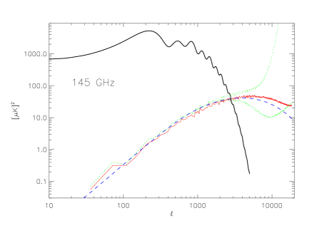
To construct the hybrid power spectrum we need to get an estimate of the cluster flux counts from the noisy recovered SZ map. We detect the clusters (above 3$\sigma$) by using SEXTRACTOR  (Bertin & Arnouts 1996) as our cluster detection algorithm. In figure (8) we show the cluster number counts recovered after SEXTRACTING  the clusters from the recovered SZ map (triangles). As a comparison, we also show the $N(S)$ curve when we use the same package (SEXTRACTOR)  but on the original SZ simulation (diamonds). The drop in counts in the faint end is due to the selection function of the survey although this selection function is “method” dependent. An optimized component separation plus cluster detection algorithm should render better results; so our results should be considered as conservative. Finally, once we have extracted the flux counts, we can use the counts (or a fit to it as shown in figure (8)) to build the hybrid power spectrum. The resultant hybrid power spectrum (for our fiducial model A in table 1) is shown as the dashed line in figure (7). One can also see that for $100<\ell<3000$, the hybrid power spectrum constructed out of ${\mathcal{N}}(S)$ very well mimics the total power spectrum from the hydro simulations. The small excess in power at $\ell\in(100,3000)$ may be due to an overestimation in the fit of the real underlying $N(S)$ curve in the bright end.

In figure (7), notice that at $\ell>3000$, the hybrid power spectrum does not agree with the actual power spectrum (for the cluster model considered here). It is at these high $\ell$-values that the effect of gas physics is dominant. Thus, once the low $\ell$ part (say $\ell<2000$) is fixed by the hybrid power spectra (which entirely depends on the observed flux counts), one can use the observed high $\ell$ part of the observed SZ power spectra to constrain cluster structure and evolution. That is, instead of using the fiducial model for the cluster parameters, we chose such cluster parameters so as to match the hybrid power spectrum to the true power spectrum.

6 Using the hybrid power spectrum to study cluster physics

In this section we come to the central point of the paper which is to present the hybrid power spectrum as a tool to study cluster physics. We first demonstrate that the hybrid power spectrum is weakly dependent on the cosmological model. From equation (5), we expect the hybrid power spectrum to be less sensitive to $\sigma_{8}$. This is evident in figure (9) where we have plotted the hybrid power spectrum while changing the cosmological parameters only. The diluted influence of the cosmological parameters on the hybrid power spectrum is striking when one compares the figures (9) & (3). At low $\ell$’s (large scales) the hybrid power spectrum is completely insensitive to the cosmological model. This is because at large scales, all the clusters behave as unresolved point sources and their power spectrum can be determined directly from the cluster flux counts (which is fixed by the observations). The power spectrum for the different cosmological models only differs at small scales where the redshift distribution of the clusters sizes (through the angular diameter distance) and fluxes (c.f equation 16) plays a part in determining the shape of the SZ power spectrum. Also, changing the cosmology will change the shape of the $N(S,z)$ surface in equation (6) but since $N(S,z)$ is normalized to $\mathcal{N}(S)$, the dependency on the cosmological model is diluted. The end result of the exercise is that the SZ power spectrum loses its strong dependence on $\sigma_{8}$ and $\Omega_{m}$. For example, comparing models A & C, we see that the two power spectra differ by a factor of two or less at $\ell>1000$, whereas if we had not used the extra information from flux counts we would get the power spectra differing by factors of four or more for a larger $\ell$-range. In essence, we have mitigated the influence of cosmology on the SZ power spectra making it suitable to study gas physics. One can still argue that we can use the hybrid power spectrum to constrain the cosmological model as it in the case of the standard power spectrum. However, in comparison to cosmology the hybrid power spectrum is now more sensitive to the cluster physics than in the case of the standard power spectrum making the hybrid power spectrum a valid tool for studies of cluster physics.

Figure 9: Sensitivity of the hybrid power spectrum to the cosmological model. The models are described in Table 1 and in the text. The hybrid power is build from the observed curve corresponding to $\sigma_{8}=0.8$ in figure (2). The fiducial model A is shown in bold line.

Figure 10: Sensitivity of the hybrid power spectrum to the cluster physics. The models are described in Table 1 and in the text. The normalization is the same as in figure (9). The fiducial model A is shown in bold line.

Next, we explore the capabilities of the hybrid power spectrum as a probe of the intracluster medium. We illustrate these capabilities in figure (10) where we show how the hybrid power spectrum behaves once we change the cluster structural parameters for a survey which gives a particular ${\mathcal{N}}(S)$ (with cosmological parameters taken from the fiducial model). A comparison of the sensitivity of the hybrid power spectrum to changes in cosmology (figure 9) and changes in the cluster parameters (figure 10) shows that the power spectrum is more sensitive to the cluster structure and evolution. On the contrary (see figures 3 & 4), for the standard total SZ power spectrum, both cosmology and cluster physics have comparable influence on the power spectrum. Thus at high $\ell$-values, for the standard power spectrum it is difficult to disentangle the effects of cosmology and cluster physics whereas for the hybrid power spectrum this degeneracy is considerably weakened. As an example, a change of 1% in $\sigma_{8}$ changes the standard power spectrum by $\approx 8$% at $\ell\approx 4000$. A similar change (1 %) in the parameter $\phi$ (temperature redshift evolution parameter) changes the standard power spectrum by $0.82$ % at $\ell\approx 4000$ whereas for the hybrid power spectrum the changes are 2.5 % (in $\sigma_{8}$) and 0.85 % (in $\phi$) respectively. A similar change in the two parameters at angular resolutions probed by ALMA (say, $\ell=30000$), changes the SZ power from 7.5 % and 2 %(standard power spectrum) to 3.8 % and 1.5 % (hybrid power spectrum) for $\sigma_{8}$ and $\phi$. Although these numbers are calculated for changes of 1 % in $\sigma_{8}$ and $\phi$, we should note that the current uncertainty in parameters like $\phi$ or $\psi$ are large (upto 100 % ). Whereas, theoretically the self-similar model predicts certain redshift dependencies (like $\phi=1$ for the M-T relation; Kaiser 1986), observationally there is still no concurring evidence (Ettori etal 2003 and references within). Uncertainties in the cosmological parameters are, however, much smaller (for example, WMAP gives an uncertainty of about 5% in $\sigma_{8}$ and 15 % in $\Omega_{M}$; Bennett etal 2003). Thus, the resulting hybrid power spectrum becomes a powerful probe of the cluster physics.

It is easy to understand the sensitivity of the hybrid power spectrum to the underlying cluster physics. To give an example, lets take the cluster temperature redshift evolution parameter $\phi$. Since the high multipoles are dominated by distance clusters (see figure 11), if $\phi$ is larger, distant clusters will appear hotter and consequently the power spectrum at small scales will be larger. This is why model A has more power at large $\ell$’s than model G. If we take model H, here the core radius is smaller for all clusters than in model A, consequently the clusters will look more compact and this will increase the power at small scales. Model J, on the other hand, will have larger cluster sizes than model A (specially at high redshifts) so its power will be smaller at small scales. Since evolution in cluster structure differentiates strongly the high redshift population w.r.t the nearby clusters, the high multipole moments of $C_{\ell}$ are very sensitive to any evolution: consequently one can strongly constrain any cluster structure evolution with the hybrid power spectrum.

The power of SZ power spectrum as a probe of cluster gas physics has already been realized (Majumdar 2001). Especially, it is seen that high $\ell$-values SZ power spectrum is very sensitive to non-gravitational processes (Komatsu & Kitayama 1999, Holder & Carlstrom 2001). This feature becomes more noticeable when the high mass clusters are subtracted from the surveys. However, the cosmology-gas physics degeneracy were not taken into account and the cosmological parameters were fixed from other observations (say, primary CMB). The novelty of this work is that we dilute the cosmological dependence of the SZ power spectrum using complementary information from the same survey itself. Moreover, we do not have to worry about cluster redshifts.

Figure 11: Contribution to the $\ell$-multipole in the SZ power spectrum as a function of the redshift of the sources Three different multipoles are shown, $\ell=500,3000,10000$. The higher the multipole $\ell$, the more dependent is the power spectrum with the high-$z$ population.

6.1 Sources of systematics

The main source of systematic error in the construction of the hybrid power spectrum comes from our partial knowledge of the ${\mathcal{N}}(S)$ curve. This partial knowledge may be due to the lack of enough statistics or a poor sensitivity in the instrument. A survey covering a small area in the sky will contain few clusters per flux bin. This will produce a noisy estimate of the ${\mathcal{N}}(S)$ curve. A small survey area will also increase the error bars due to cosmic variance. In particular, the latter can have a significant effect in the high flux interval since we expect bright clusters to be less common than the faint ones. A lack of bright clusters in the sample (or similarly an underestimated ${\mathcal{N}}(S)$ curve at high fluxes) will lead to an underestimated hybrid power spectrum in large scales (small $\ell$’s). Consequently, by subtracting the hybrid power spectrum from the total (observed) power spectrum one can get a biased estimate of the correlation term if the ${\mathcal{N}}(S)$ curve is not correctly estimated in the high flux regime. As an immediate example, we see this error in estimation has given us hybrid power spectrum with slightly more power than the total power spectrum at large scales (see figure (7)). One can try to bypass this systematic by using a fit to the ${\mathcal{N}}(S)$ curve to high fluxes. However, in order to have a good fit it is necessary to have a large number of bright clusters. On the other hand, a poor sensitivity of the instrument will reduce the number of faint clusters detected in the survey. The faint clusters will contribute to the hybrid power spectrum in the high $\ell$ regime (where the sensitivity of the hybrid power spectrum with the cluster physics is more relevant). Moreover, the cluster catalog (and hereby the ${\mathcal{N}}(S)$ curve) will be the product of a processing of the raw data (e.g component separation) which usually introduce a selection function in the cluster catalog. Understanding the selection function is fundamental specially at the faint end of the catalog where the selection function is expected to change dramatically. Usually, one should fit the ${\mathcal{N}}(S)$ curve only using those data points for which the selection function is well understood. Then one can extrapolate the fit to lower (or higher) fluxes and build $C^{H}_{\ell}$ from the fitting.

7 Discussion and summary

In the previous sections we have demonstrated that cosmology as well as cluster gas structure and evolution simultaneously shapes the thermal SZ power spectrum from clusters of galaxies. The power spectrum depends strongly on certain cosmological parameters (like $\sigma_{8}$) and on any evolution, if present, thus leading to a cosmology-gas physics degeneracy. One can take priors from external observations, for example fix the cosmological model from primary CMB, and use the power spectrum to probe gas physics. However, it is possible to combine complimentary information from the same survey itself to mitigate the influence of cosmology in order to study gas physics.

To do so, we have formulated a different way of looking at the SZ power spectrum by constructing the hybrid power spectrum. Given that any future large yield SZ survey would also detect many thousands of clusters, we would have a flux counts of the objects detected in the survey. At the same time, temperature fluctuations from all the survey pixels would be used to construct the total SZ power spectrum. We have shown that one can rewrite the Poisson part of the SZ power spectrum using the information available from the SZ flux counts. Since the Poisson power spectrum dominates, in general, over the clustering power spectrum, the resultant hybrid power spectrum represents the total SZ power spectrum sufficiently well up to $\ell\sim 2000$. We also used results from numerical simulations to test and verify our analytical results. Since both the SZ power spectrum and the flux counts represent the same underlying cosmology, the hybrid power spectrum is, in essence, normalized to the background cosmology. Once the cosmology-gas physics degeneracy is diluted, we are left with modeling of the gas physics to understand the observed total SZ power spectrum at higher multipoles.

We have used a simple model of the cluster gas structure and evolution as well analytical results for the mass function in our analytical model. This is sufficient for the present work which is exploratory in nature. Needless to say, practical application of the method would need better modeling of the complex cluster structure using N-body hydro simulations or with more complicated analytical models (suitable to fit simulation results). Cosmological simulations of large yield of clusters mimicking upcoming surveys are still naive in the sense that they still need some sort of phenomenological approach to model the gas physics (especially non-adibaticity) and has to make simplifying assumptions as to the cluster structure. At the same time simulating any non-standard cluster evolution is non-trivial and either done too simplistically or is put in by-hand in the simulations. It is this very cluster structure and evolution that we are able to probe by studying the SZ power spectrum at high $\ell$-values. Note, that in figure (7), at multipoles ($\ell>2000$) the hybrid power spectrum defers from the actual power spectrum. This, of course, should be the case since the cluster structure (c.f. equations (10) & (11)) used in constructing $C^{H}_{l}$ is very different from the gas physics used in the SZ N-body simulations. However, it must be kept in mind that a part of the difference may arise from increase in power at high $\ell$’s due to presence of substructures in the clusters which are naturally captured in any N-body simulations but not modeled analytically.

The ability to construct $C^{H}_{l}$ depends crucially on our capability to get the cluster flux counts. The main source of systematic error in the construction of the hybrid power spectrum comes from our partial knowledge of the ${\mathcal{N}}(S)$ curve. This partial knowledge may be due to the lack of enough statistics or a poor sensitivity in the instrument. It is also important to understand that processing of the raw data can introduce a selection function in the cluster catalog. Usually, one should fit the ${\mathcal{N}}(S)$ curve only using those data points for which the selection function is well understood and then extrapolate the fit to lower (and/or higher) fluxes. This extrapolation will have little effect in the constructed hybrid power spectrum if the survey is large enough such that it contains enough bright clusters and if its sensitivity is good enough to recover clusters with fluxes as low as a few mJy (say, at 145 GHz). Future SZ cluster surveys (like ACT/SPT/APEX-SZ) satisfy both these conditions such that the hybrid power spectrum can be a useful tool in these surveys.

The main conclusion of this work can be summarized by comparing figures (9 & 10) with figures (3 & 4). By using the hybrid power spectrum instead of the standard power spectrum, one can dilute the dependency of the power spectrum on the cosmological model and concentrate on studies of the cluster physics. The precision in the determination of the cosmological parameters has increased dramatically in recent times. However, much uncertainties remain in studies of cluster physics. Better handle on cluster structure and evolution becomes even more challenging when one takes in to account the cosmology-gas physics degeneracy in any such studies. The hybrid power spectrum helps to soften this problem by diluting much of this degeneracy.

The prospect of probing gas physics using SZ power spectrum would depend on our ability to measure the SZ power spectrum as very high $\ell$-values. This sub arc-min scale has the distinct advantage of the primary CMB contribution being negligible. However one has to be careful in eliminating other possible sources of secondary CMB anisotropies that may introduce further systematic uncertainties. In multifrequency experiments, an appropriate SZ reconstruction algorithm should be able to recover the true SZ power spectrum up to the resolution limit of the experiment

Finally, all future high sensitivity SZ observations have to tackle the noise introduced by unresolved point sources. The spectral dependence of the thermal SZ effect would be helpful in eliminating many of such systematics. Although not studied in this work, another interesting application of the hybrid power spectrum is to perform consistency checks on the excess in power in single frequency CMB experiments. By this we mean that future CMB experiments will observe an excess in the power spectrum of CMB fluctuations at $\ell>2000$. This excess will be due in part to galaxy clusters, and in part to non-removed point sources (see figure 2 in White & Majumdar 2003). Now, at $\ell\sim 2000$ the hybrid power spectrum is a decent representation of the total SZ power spectrum without worrying much about cluster physics. If there is an estimation of the $\mathcal{N}(S)$ curve for the survey, then one can estimate SZ power due to clusters at $\ell\sim 2000$. Any excess power can be interpreted as due to unresolved point sources.

In spite the stringent requirements needed to make SZ observations from the upcoming surveys probe of cluster physics, the rewards reaped would undoubtedly be great. In addition to new high resolution targeted observations, the statistical study of the SZ sky from cosmological distribution of clusters may provide the next leap in the study of the structure and evolution of galaxy clusters.

8 Acknowledgments

The authors would like to thank Martin White for providing the SZ maps and the group catalogs. We also would like to thank Max Tegmark, Ue-Li Pen, Gil Holder, Martin White and Maija Jespersen for discussions and suggestions. The work of JMD was supported by the David and Lucile Packard Foundation and the Cottrell Foundation.

Appendix A
The hybrid power spectrum for X-ray surveys

The computation of the hybrid power spectrum for the case of X-ray surveys can be done following the same procedure as in the SZ case. We start with a measured cluster number counts, ${\mathcal{N}}(S)$ (where now the fluxes are given in ergs s^-1 cm^-2). The fluxes can be connected with the mass through the equations;

$$S=\frac{L_{x}}{4\pi D_{l}^{2}}$$ (20)

$$L_{x}=L_{o}M^{\alpha}(1+z)^{\phi}$$ (21)

where $L_{x}$ is the cluster X-ray luminosity and $D_{l}$ is the luminosity distance. The constant $L_{o}$ will contain all the units and the conversion factors (band correction, conversion between cts/s and ergs/s). Equation (21) will play the same role as the $T-M$ relation in the case of a SZ survey. The final ingredient we need to compute the X-ray hybrid power spectrum is the function $f(\ell,M,z)$ which will differ to the one described in section 3. For the case of X-ray images, the 2D profile of a cluster will look different since is proportional to the integral along the line of sight of the density squared. The fourier transforms of these 2D profiles can be fitted rendering;

$$f(\ell,M,z)=\frac{1}{2}\left(\exp(-\xi_{l,r_{c}})+\exp(-\sqrt{\xi_{l,r_{c}}})\right)$$ (22)

with,

$$\xi_{l,r_{c}}=l^{2}r_{c}^{1.5/(0.815+0.35r_{c})}$$ (23)

where the core radius, $r_{c}$, is given in rads (see Diego et al. 2003).

References

- [1] Bahcall, N. A. & Fan, X. 1998, ApJ, 504, 1
- [2] Barbosa, D., Bartlett, J. G., Blanchard, A. & Oukbir, J. 1996, A&A, 314, 13
- [3] Barbosa, D., Bartlett, J. G. & Blanchard, A. 1998, APSS, 261, 277
- [4] Bartlett, J. G. 2000, astro-ph/0001267.
- [5] Bennett, C. L. et al, 2003, ApJ, 138, 1
- [6] Bertin, E. & Arnouts, S. 1996, ApJS, 117, 393.
- [7] Bond, J. R. et al., astro-ph/0205386.
- [8] Bouchet F., & Gispert R. 1999, NewA, 4, 443.
- [9] Cooray, A. 2000, PRD, 62j3506C.
- [10] Cooray, A., Hu, W. & Tegmark, M., 2000, ApJ, 540, 1.
- [11] Cooray, A. & Sheth R., Physics Reports, 372, 1
- [12] da Silva, A. C., Barbosa, D., Liddle, A. R. & Thomas, P. A. 2000, MNRAS, 317, 37
- [13] da Silva, A. C., Kay, S. T., Liddle, A. R., Thomas, P. A., Pearce, F. R. & Barbosa, D., 2001, ApJL, 561, 15
- [14] Delabrouille J., Cardoso J.-F., Patanchon G. 2003, MNRAS, 346, 1089.
- [15] Diego, J. M., Martínez-González, E., Sanz, Cayón, L. & Silk, J. 2001, MNRAS, 325, 1533
- [16] Diego, J. M., Martínez-González, E., Sanz, J. L., Benitez, N. & Silk, J. 2002, MNRAS, 331, 556
- [17] Diego, J. M., Sliwa, W., Silk, J., Barcons, X. 2003, MNRAS, 344,951
- [18] Ettori, S., Tozzi, P., Borgani, S. & Rosati, P., 2003, astro-ph/0312239
- [19] Finoguenov, A., Reiprich, T. H., & Böhringer, H. 2001, A&A, 368, 749
- [20] Henry, J. P. 1997, ApJ, 489, L1
- [21] Hobson M.P., Jones A.W., Lasenby A.N., & Bouchet F.R. 1998, MNRAS, 299, 895.
- [22] Holder, G. P. & Carlstrom, J. E. 2001, ApJ, 558, 515
- [23] Hu, W. & Kravtsov, A. V. 2003, ApJ, 584, 702
- [24] Jenkins, A., Frenk, C. S., White, S. D. M., Colberg, J. M., Cole, S., Evrard, A. E., Couchman, H. M. P., & Yoshida, N. 2001, MNRAS, 321,372
- [25] Kaiser, N., 1986, MNRAS, 222, 323
- [26] Knox, L., Holder, G. & Church, S., 2003, astro-ph/0309643
- [27] Komatsu E., & Kitayama T., 1999, ApJ, 526, L1.
- [28] Komatsu E., & Seljak U., T., 2002, MNRAS, 336, 1256.
- [29] Levine, E. S., Schulz, A. E., & White, M. 2002, ApJ, 577, 569
- [30] Lima. M. & Hu, W.. 2004, astro-h/0401559
- [31] Maino et al. (more than 8 authors). 2002, MNRAS, 334, 53.
- [32] Majumdar, S. 2001, ApJ, 555, L7
- [33] Majumdar, S. & Mohr, J. J. 2003a, ApJ, 585, 603
- [34] Majumdar, S. & Mohr, J. J. 2003b, astro-ph/0305341
- [35] Martínez-González, E., Diego, J. M., Vielva, P. & Silk, J., 2003, MNRAS, 345, 1101
- [36] Mo, H. J. & White, S. D. M. 1996, MNRAS, 282, 347
- [37] Press W.H., Schechter P., 1974, ApJ, 187, 425
- [38] Refregier, A., Komatsu, E., Spergel, D. N. & Pen, U. 2000, PRD, 61l3001R
- [39] Refregier, A. & Teyssier, R., 2002, PRD, 66d3002R
- [40] Sadeh, S. & Repaheli, Y., 2004a, New Astronomy, 9, 159
- [41] Sadeh, S & Rephaeli, Y, 2004b, astro-ph/0401033
- [42] Seljak, U., Burwell, J. & Pen, U. 2001, PRD, 63f3001S
- [43] Sheth, R. K. & Tormen, G. 1999, MNRAS, 308, 119
- [44] Springel, V., White, M. & Hernquist, L. 2001, ApJ, 549, 681
- [45] Verde, L., Kamionkowski, M., Mohr, J. J. & Benson, A. J. 2001, MNRAS, 321, L7
- [46] Viana, P. T. P. & Liddle, A. R. 1999, MNRAS, 303, 535
- [47] Wang, L. & Steinhardt, P. J. 1998, ApJ, 508, 483
- [48] Weller, J., Battye, R., & Kniessl, R. 2002, PRL, 88, 1301.
- [49] White, M. 2003, ApJ, 597, 650
- [50] White, M & Majumdar, S., 2003, astro-ph/0308464, accepted ApJ
- [51] Zhang, P. & Pen, U, 2001, ApJ, 549, 18
- [52] Zhang, P., Pen, U & Wang, B. 2002, ApJ, 577, 555
- [53] Zhang, P., Pen, U & Trac, H. 2004, astro-ph/0402115