The Gemini Deep Deep Survey: I. Introduction to the Survey, Catalogs and Composite Spectra

Abstract

The Gemini Deep Deep Survey (GDDS) is an ultra-deep ($K<20.6$ mag, $I<24.5$ mag) redshift survey targeting galaxies in the “redshift desert” between $1<z<2$. The primary goal of the survey is to constrain the space density at high redshift of evolved high-mass galaxies. We obtained 309 spectra in four widely-separated 30 arcmin² fields using the Gemini North telescope and the Gemini Multi-Object Spectrograph (GMOS). The spectra define a one-in-two sparse sample of the reddest and most luminous galaxies near the $I-K$  vs. $I$  color-magnitude track mapped out by passively evolving galaxies in the redshift interval $0.8<z<1.8$. This sample is augmented by a one-in-seven sparse sample of the remaining high-redshift galaxy population. The GMOS spectrograph was operating in a Nod & Shuffle mode which enabled us to remove sky contamination with high precision, even for typical exposures times of 20–30 hours per field. The resulting spectra are the deepest ever obtained. In this paper we present our sample of 309 spectra, along with redshifts, identifications of spectral features, and photometry. This makes the GDDS the largest and most complete infrared-selected survey probing the redshift desert. The 7-band ($VRIzJHK_{s}$) photometry is taken from the Las Campanas Infrared Survey. The infrared selection means that the GDDS is observing not only star-forming galaxies, as in most high-redshift galaxy surveys, but also quiescent evolved galaxies. In our sample, we have obtained 225 secure redshifts, 167 of which are in the redshift interval $0.8<z<2$. About 25% of these show clear spectral signatures of evolved (pure old, or old + intermediate-age) stellar populations, while 35% of show features consistent with either a pure intermediate-age or a young + intermediate-age stellar population. About 29% of the galaxies in the GDDS at $0.8<z<2$ are young starbursts with strong interstellar lines. A few galaxies show very strong post-starburst signatures. Another 55 objects have less secure redshifts, 31 of which lie in the redshift interval $0.8<z<2$. The median redshift of the whole GDDS sample is $z=1.1$. Spectroscopic completeness varies from a low of $\sim 70\%$ for red galaxies to $>90\%$ for blue galaxies. In this paper we also present, together with the data and catalogs, a summary of the criteria for selecting the GDDS fields, the rationale behind our mask designs, an analysis of the completeness of the survey, and a description of the data reduction procedures used. All data from the GDDS are publicly available.

1 INTRODUCTION

The Gemini Deep Deep Survey (GDDS) is an infrared-selected ultra-deep spectroscopic survey probing the redshift range $0.8<z<1.8$. It is designed to target galaxies of all colors at high redshift with an emphasis on the reddest population. The survey is designed with the following scientific goals in mind: (1) Measurement of the space density and luminosity function of massive early-type galaxies at high redshift. (2) Construction of the volume-averaged stellar mass function in at least three mass bins and two redshift bins over the target redshift range. (3) Measurement of the luminosity-weighted ages and recent star-formation histories of $\sim 50$ evolved galaxies at $z>1$ (cf. Dunlop et al. 1996). The over-arching goal of the survey is to use these sets of observations to test hierarchical models for the formation of early-type galaxies. Many studies (see Ellis (2001) for a recent review) have probed the evolving space density of early-type systems and it is now clear that the number density of early-types does not evolve rapidly out to $z=1$, as once predicted by matter-dominated models (see Ellis 2001 for a review). However, $\Lambda$-dominated cosmologies push back the formation epoch of most early-type systems out to at least $z=1$ even in a hierarchical picture. Alternative theories for the origin of early-type galaxies (e.g. high-z monolithic collapse vs. hierarchical formation from mergers) now start to become readily distinguishable at exactly the redshift ($z=1$) where spectroscopy from the ground becomes problematic (Kauffmann et al. 1998).

Our focus on the redshift range $0.8<z<1.8$ is motivated by two additional considerations. Firstly, the star-formation histories of individual galaxies in this redshift range have been very poorly explored. We do not even know whether most red objects in this range are old and quiescent, or very young and active and heavily reddened by dust. Distinguishing between these two possibilities requires high signal-to-noise in the continuum so that the characteristic photospheric features of evolved stars become evident, but most work in this redshift range has focused on emission lines. Secondly, and irrespective of model predictions, this redshift range appears to correspond to the peak epoch of galaxy assembly inferred by integrating under the ‘Madau/Lilly plot’, an observationally-defined diagram quantifying the volume-averaged star-formation history of the Universe as a function of redshift (Madau et al. 1996; Lilly et al. 1996; Steidel et al. 1999). The high-redshift tail of this plot is subject to large and uncertain dust and surface-brightness corrections, and remains rather poorly determined, and recent observations have pushed back the peak of star-formation, showing a broad maximum in redshift (for a summary of the observational situation, see Figure 2 in Nagamine et al. 2003). However, the integral under the Madau/Lilly plot is simply the total mass assembled in stars per unit volume, so by measuring this quantity directly in the GDDS we can undertake a basic consistency check of the overall picture inferred from global star-formation history and luminosity density diagrams.

Spectroscopy of galaxies in the redshift range we seek to probe suffers from technical challenges brought on by the lack of strong spectral features at visible wavelengths. The redshift range $1<z<2$ has come to be known as the “redshift desert”, in reference to the paucity of optical redshifts known over this interval. Fortunately, it is now becoming clear that redshifts and diagnostic spectra can be obtained using optical spectrographs in this redshift range, by focusing on rest-frame UV metallic absorption features. Good progress is now being made in obtaining redshifts for UV-selected samples in the redshift desert using the blue-sensitive LRIS-B spectrograph on the Keck telescope (Steidel et al. 2003; Erb et al. 2003). However, UV-selected surveys are biased in favor of high star-formation rate galaxies, and the passive red galaxies with high mass-to-light ratios that are missed by UV-selection could well dominate the high-$z$ galaxy mass budget, motivating deep $K$-selected surveys such as the VLT K20 survey (Cimatti et al. 2003), and ultra-deep small area surveys such as FIRES (Franx et al. 2003). We refer the reader to Cimatti et al. (2004) for an excellent summary of recent results obtained from infrared-selected surveys probing high-redshift galaxy evolution. The GDDS is designed to build upon these results.

Because their rest-UV continuum is so weak, determining the redshifts of passive red galaxies at $z\sim 1.5$ with 8m-class telescopes presently requires extreme measures. Ultra-deep ($>10$ hour) integration times and Poisson-limited spectroscopy are required in order to probe samples of red galaxies with zero residual star-formation and no emission lines. This poses a severe problem, because MOS spectroscopy with 8m-class telescopes is generally not Poisson-limited unless exposure times are short (less than a few hours). The main contributors to the noise budget are imperfect sky subtraction and fringe removal. At optical wavelengths, both of these problems are most severe redward of 7000Å, where most of the light from evolved high redshift stellar populations is expected to peak. To mitigate against these effects, the Gemini Deep Deep Survey team has implemented a Nod & Shuffle sky-subtraction mode (Glazebrook et al. 2001; Cuillandre et al. 1994; Bland-Hawthorn 1995) on the Gemini Multi-Object Spectrograph (Murowinski et al. 2003; Hook et al. 2003). This technique is somewhat similar to beam-switching in the infrared, and allows sky subtraction and fringe removal to be undertaken with an order of magnitude greater precision than is possible with conventional spectroscopy.

In order to undertake an unbiased inventory of the high-redshift galaxy population, the GDDS is $K$-band selected to a sufficient depth ($K=20.6$ mag) to reach $L^{\star}$ throughout the $1<z<2$ regime. IR-selected samples that do not reach to this $K$-band limit are limited primarily to the $z<1$ epoch, while samples that go substantially deeper outrun the capability of ground-based spectroscopic follow-up for the reddest objects, and once again become biased. The standard definition for an ‘Extremely Red Galaxy’, or ERG, is $I-K\gtrsim 4$, a threshold which roughly corresponds to the expected color of an evolved dust-free early-type galaxy seen at $z\sim 1$. As will be shown below, the effective limit for obtaining absorption-line redshifts for red galaxies with weak UV continua is about $I=25$ mag with an 8m telescope. (Our GDDS spectroscopy — the deepest ever undertaken — has a magnitude limit of $I=24.5$ mag). Therefore at present it is only just possible to obtain a nearly complete census of redshifts for all evolved red objects in a $K\sim 21$ imaging survey. Our strategy with the GDDS is to go deep enough to allow redshifts to be obtained for $L_{\star}$ galaxies irrespective of star-formation history at $z\sim 1.5$, while simultaneously covering enough area to minimize the effects of cosmic variance. Our sampling strategy (based on photometric redshift pre-selection to eliminate low-$z$ contamination) is different from that adopted by most other redshift surveys. In terms of existing surveys, the K20 survey (Cimatti et al. 2003) is probably the closest benchmark comparison to the GDDS, although the experimental designs are very different, making the K20 and GDDS surveys quite complementary. The K20 survey has about twice as many redshifts as the GDDS, but because K20 survey does not preferentially select against low-redshift objects, most of these are at $z<1$. The GDDS has between two and three times as many redshifts as K20 in the interval $1.2<z<2$ (the precise number depending on the minimum acceptable redshift confidence class), and has a higher median redshift ($z\sim 1.1$ vs. $z\sim 0.7$). The GDDS also goes about 0.6 mag deeper in $K$ and has over twice the area (121 square arcmin in four widely-separated site-lines in the GDDS vs. 52 square arcmin in two widely-separated site-lines in K20).

A plan for this paper follows. In §2 we describe our experimental design, with a particular focus on how our targets were selected from the Las Campanas Infrared Survey. In §3 we outline our observing procedure, but defer the details of the Nod & Shuffle mode that are not specific to the GDDS to an Appendix. (Nod & Shuffle on the Gemini Multi-Object Spectrograph was implemented for use on the GDDS but is now a common-user mode. Since many observers may wish to use the mode themselves in contexts unrelated to faint galaxy observations, the Appendices to this paper will act as a stand-alone reference to using the mode on Gemini). In Section 4 we summarize the data obtained from the GDDS, both graphically and as a series of tables. Composite spectra obtained by co-adding similar spectra are presented in Section 5. We used these composite as templates to obtain redshifts in the GDDS, but others may wish to apply them to their own work for other purposes. Some implications from the data obtained are discussed and our conclusions given in Section 6. The major results from the GDDS will be presented in three companion papers.

Appendix A describes the operation of the Nod & Shuffle mode on the Gemini Multi-Object Spectrograph (Hook et al. 2003) (GMOS) in the context of the GDDS. A more general description of the implementation of the mode will be given in Murowinski et al. (in preparation). Appendix B describes how the two-dimensional data from the GDDS were reduced. Appendix C describes how the final one-dimensional spectra were extracted from the two-dimensional data.

The catalogs presented in this paper, as well as reduced spectra for all galaxies in the GDDS, are available in electronic form as a digital supplement to this article. All software described in this paper, as well as auxiliary data, are publicly available (in both raw and fully reduced form) from the central GDDS web site located at http://www.ociw.edu/lcirs/gdds.html.

Throughout this paper we adopt a cosmology with $H_{0}$=70 km/s/Mpc, $\Omega_{M}=0.3$, and $\Omega_{\Lambda}=0.7$.

2 EXPERIMENTAL DESIGN

All galaxies observed in the GDDS were taken from seven-filter ($BVRIz^{\prime}JK$) photometric catalogs constructed as part of the one square-degree Las Campanas Infrared survey (LCIR survey; McCarthy et al. 2001; Chen et al. 2002; Firth et al. 2001). The GDDS can be thought of as a sparse-sampled spectroscopically defined subset of the LCIR survey. The GDDS is comprised of four Gemini Multi-Object Spectrograph (GMOS) integrations, each with exposure times between 21 and 38 hours. Each GDDS field lies within a separate LCIR survey equatorial field. (The LCIR survey fields chosen were SSA22, NOAODW-Cetus, NTT-Deep, and LCIR 1511; the reader is referred to Chen et al. 2002 for information on the LCIR survey data available in these fields). Since the publication of Chen et al. 2002 additional imaging data has been acquired for these fields. Deep $K_{s}$, and in some cases, J imaging supplements the VVRIz’H data discussed in Chen et al. The 5$\sigma$ completeness limit of the LCIR survey fields is K${}_{s}=20.6$ mag (on the Vega scale). The 5.5′x 5.5′ GMOS field of view is small relative to even a single 13′x 13′ ‘tile’ of the LCIR survey (four such tiles constitute a single LCIR survey field). We therefore had considerable freedom to position the GMOS pointing within each LCIR survey field in areas which avoided very bright foreground objects and which had suitable guide stars proximate to the fields. We were also careful to pick regions in each field where the number of red galaxies was near the global average (i.e. we tried to avoid obvious over-densities and obvious voids; our success in achieving this will be quantified below). The four GMOS fields in our survey will be referred to as GDDS-SA22, GDDS-SA02, GDDS-SA12 and GDDS-SA15 for the remainder of this paper and in subsequent papers in this series. Taken together, these survey fields cover a total area of 121 square arcmin. The locations of each field and the total exposure time per spectroscopic mask are given in Table 1. Finding charts for individual galaxies within the GDDS fields are shown in Figures 1–4.

Table 1: Overview of Observations

Field	RA (J2000)	Dec (J2000)	Target slits	Mask Definition File	Exposure Time(s)
GDDS-SA02	02:09:41.30	-04:37:54.0	59	GN2002B-Q-1-1.fits	75600
GDDS-SA12	12:05:22.17	-07:22:27.9	61	GN2003A-Q-1-1.fits	18000
”	12:05:22.17	-07:22:27.9	74	GN2003A-Q-1-3.fits	57600
GDDS-SA15	15:23:47.83	-00:05:21.1	59	GN2003A-Q-1-5.fits	70200
GDDS-SA22	22:17:41.0	+00:15:20.0	83	GN2002BSV-78-14.fits	48600
”	22:17:41.0	+00:15:20.0	62	GN2002BSV-78-15.fits	90000

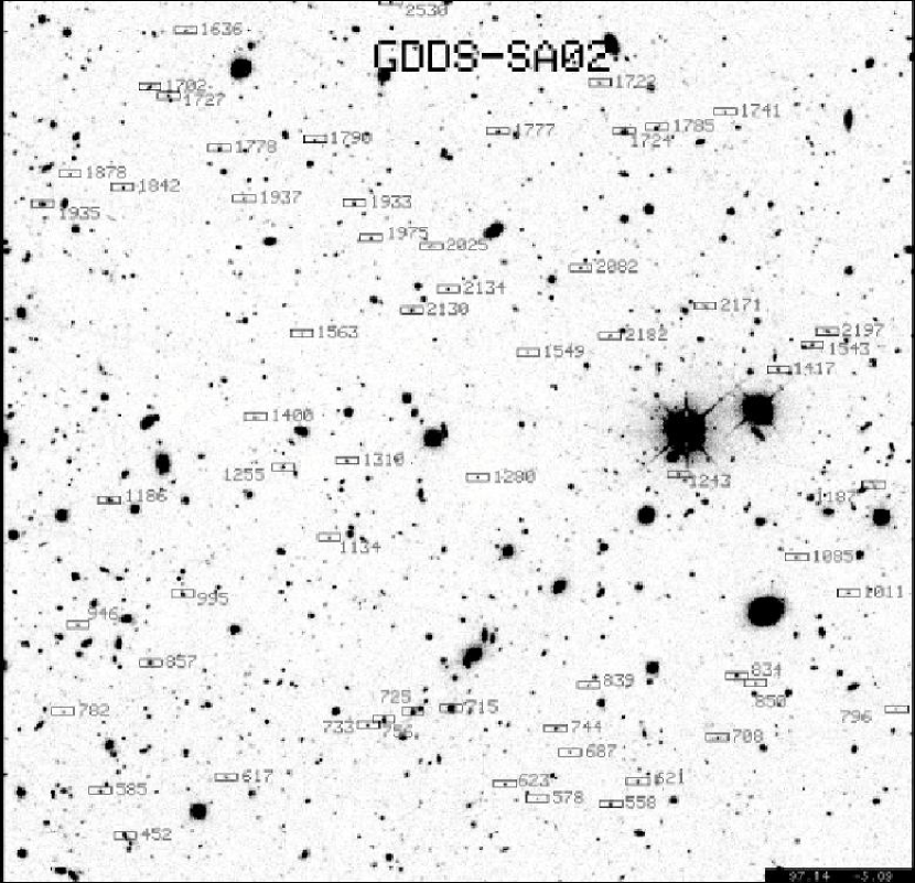
Figure 1: Labeled finding chart for the GDDS-SA02 field. The field size is 5.5′x 5.5′. The central coordinates for this field are given in Table 1. Numeric object labels correspond to the ID’s in Tables 4 and 5. The background image is a 180 min $I$-band image obtained with the KPNO 4m MOSIAC imager as part of the LCIR survey.

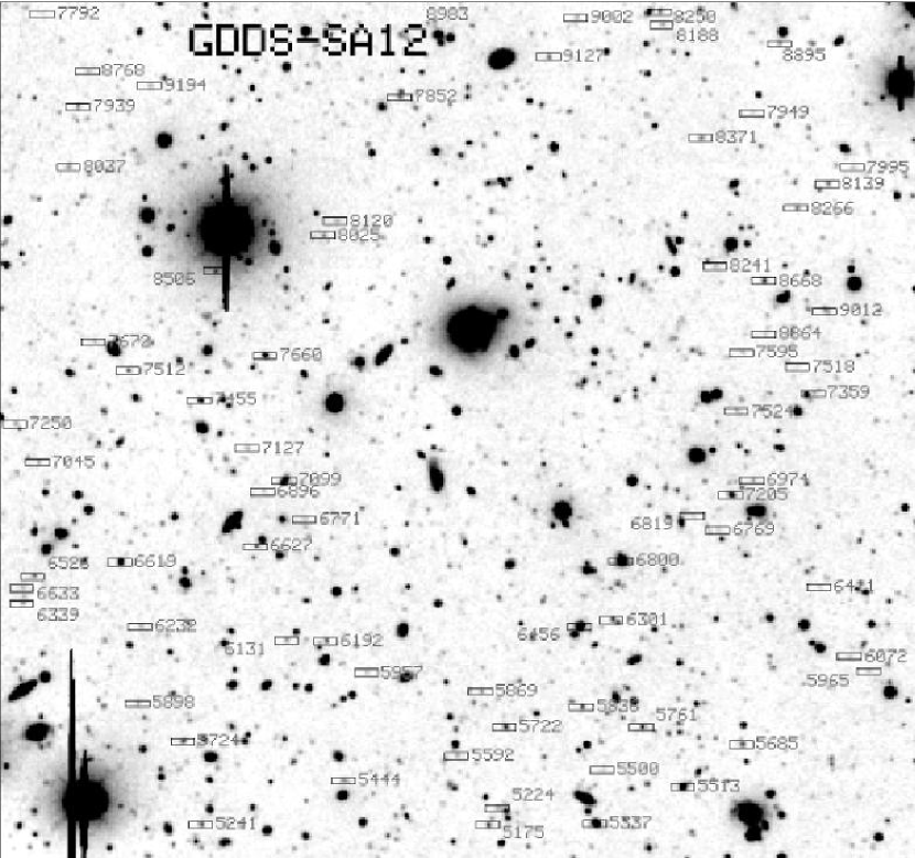
Figure 2: Labeled finding chart for the GDDS-SA12 field. The field size is 5.5′x 5.5′. Central coordinates for this field are given in Table 1. Numeric object labels correspond to the ID’s in Tables 4 and 5. The background image is a 180 minute $I$-band exposure taken with the BTC on the CTIO 4m telescope as part of the LCIR imaging survey.

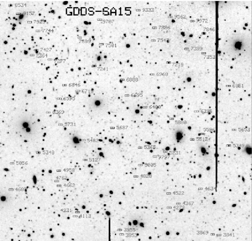
Figure 3: Labeled finding chart for the GDDS-SA15 field. The field size is 5.5′x 5.5′. Central coordinates for this field are given in Table 1. Numeric object labels correspond to the ID’s in Tables 4 and 5. The background is a 180 minute $I$-band image obtained with the BTC on the CTIO 4m as part of the LCIR survey.

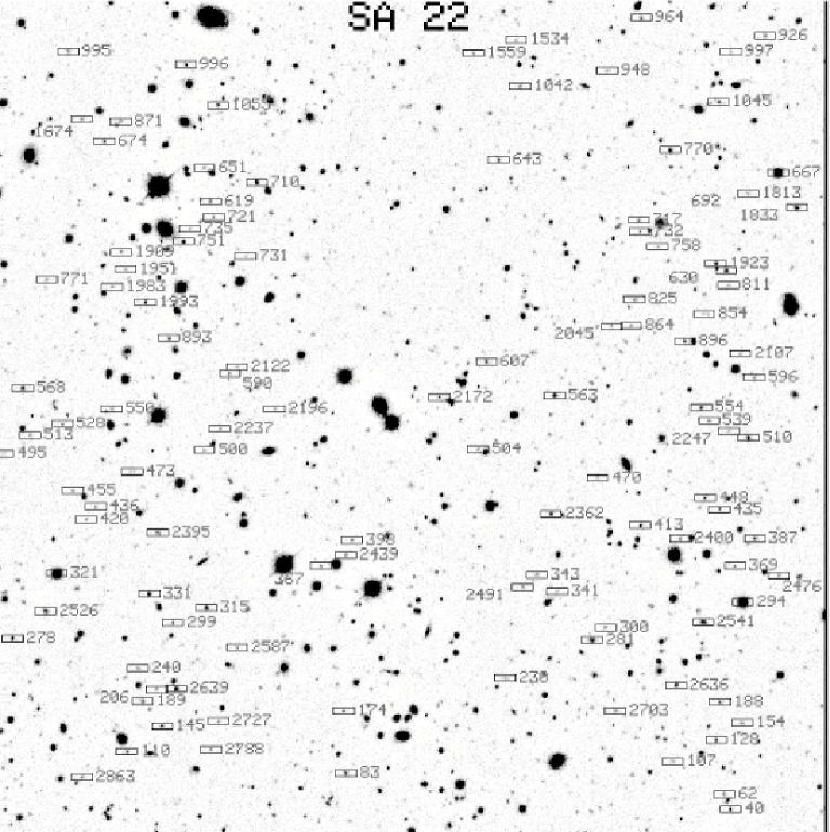
Figure 4: Labeled finding chart for the GDDS-SA22 field. The field size is 5.5′x 5.5′. Central coordinates for this field are given in Table 1. Numeric object labels correspond to the ID’s in Tables 4 and 5. The background image is a 120 minute $I$-band exposure obtained with the 12k mosaic camera on the CFHT kindly provided to us by P. Stetson.

At $z=1.2$ (the median redshift of our survey), the 5.5 arcmin angle subtended by each GMOS field of view corresponds to a physical size of 2.74 Mpc. The total comoving volume in the four GDDS ‘pencil beams’ over the redshift interval $0.8<z<1.8$ (the range over which $L^{\star}$ galaxies would be detected in the GDDS) is 320,000 ${\rm Mpc}^{3}$. Over this volume the effects of cosmic variance on random pointings is quite significant, especially for the highly clustered red objects in our survey whose correlation length is large ($\sim 10h^{-1}$ Mpc; McCarthy et al. 2001; Daddi et al. 2000). Fortunately, completely random pointings are unnecessary, because the global statistical properties of the the LCIR survey (the GDDS’ parent population) are well defined. As mentioned earlier, we took advantage of this extra information when selecting our GDDS fields by ensuring that the areal density of red ($I-K>4$) galaxies was close to the ensemble average of such galaxies in the LCIR survey. Figure 5 compares the density contrast of red galaxies in each of our fields to the histogram obtained by measuring this same quantity in a series of random 5.5′ x 5.5′ boxes overlaid on the 26′ x 26′  LCIRS field from which the corresponding GDDS field was selected. In GDDS-SA15 and GDDS-SA02 the number of red galaxies is essentially identical to the median number expected from the parent population. The number of red galaxies in GDDS-SA22 is somewhat lower than the global median, while the number in GDDS-SA12 is somewhat higher than the global median. Averaged over the four fields, the areal density of red systems in the GDDS is close to the typical value expected.

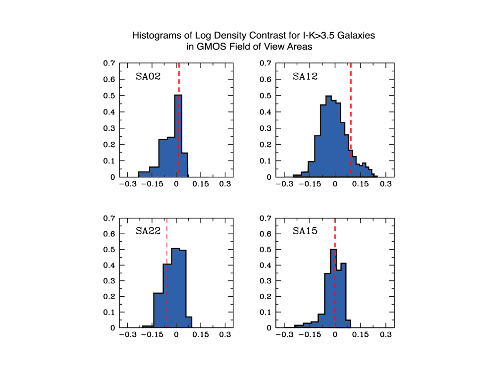
Figure 5: The density contrast of $(I-K)>4$ galaxies in each 5.5 arcmin x 5.5 arcmin GDDS field (dashed vertical line) compared with the histogram obtained by measuring this quantity in a series of random boxes overlaid on the 26′ x 26′  LCIRS field from which the GMOS field was selected.

The areal density of galaxies in the LCIR Survey with photometric redshifts in the range $1<z<2$ and $I<24.5$ mag is about 8 arcmin^-2, corresponding to about 250 galaxies in a typical GMOS field of view. Since this is about a factor of four larger than can be accommodated in a single mask with GMOS, even in in Nod & Shuffle microslit mode, it is impossible to target every candidate $1<z<2$ galaxy with a single mask. On the other hand, to reach our required depth on Gemini requires around 100ks of integration time, which means it is not practical to obtain many masks per field in a single semester. Fortunately, the areal density of red galaxies with $I-Ks>4$ and $I<24.5$ is only $\sim 1$ arcmin^-2, so it is at least possible (in principle) to target all red galaxies in the appropriate redshift range. We therefore adopted a sparse-sampling strategy based on color, apparent magnitude, and photometric redshift in order to maximize the number of targeted galaxies occurring in our desired redshift range, with a particular emphasis on red galaxies. Targets were selected from the photometric catalogs on the basis of $K_{s}$ and $I$ magnitudes measured in $3^{\prime\prime}$ diameter apertures. Complete photometric catalogs for our sample will be presented below.

Our sparse-sampling strategy is summarized graphically in Figure 6. Each panel in this figure shows two-dimensional histograms of different quantities within the parameter space defined by our $(I-K_{s})$ vs. $I$ photometry. The dashed line at the bottom-right corner of each panel denotes the region in this parameter space below which the $K_{s}$ band magnitudes of galaxies become fainter than the formal 5$\sigma$ $K_{s}=20.6$ magnitude limit of the survey. Non-detections have been placed at the detection limit in our master data tables (presented below), so the bunching up of galaxies in the boxes intersected by this line is mostly artificial (the counts are inflated by blue galaxies undetected in $K_{s}$).

The top-left panel of Figure 6 shows the distribution in color-magnitude space of all galaxies in a 554.7 square arcmin subset of the LCIRS, corresponding to the parent ‘tiles’ of the LCIRS from within which our GDDS fields were chosen. The labeled track on this panel shows the expected position as a function of redshift of an M^⋆ (assumed to be $M_{K}=-23.6$) galaxy formed in a 1 Gyr burst at redshift $z=10$. The position of this model old galaxy at several observed redshifts between $z=1.7$ and $z=0.7$ are marked with red dots and are labeled. Note the good agreement between the locus defined by the reddest galaxies in the LCIRS and the model track. Most galaxies should be bluer than our extreme old galaxy model, suggesting that the optimal area for a mass-limited survey targeting $0.8<z<1.8$ should be the region defined by $\{22<I<24.5,\ 3<(I-K_{s})<5\}$. This basic conclusion is borne out by a comparison with the full photometric redshift distribution computed from our seven-filter photometry, shown in the top-right panel of Figure 6.

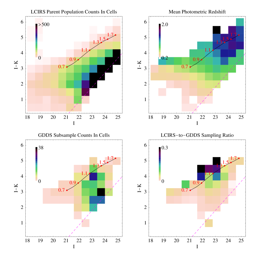
Figure 6: (Top left:) A two-dimensional histogram showing the distribution in color-magnitude space of all galaxies in a 554.7 square arcmin subset of the LCIRS, corresponding to the parent ‘tiles’ of the LCIRS from within which our GDDS fields were chosen. The labeled track on this panel shows the expected position as a function of redshift of an M^⋆ (assumed to be $M_{K}=-23.6$) galaxy formed in a 1 Gyr burst at redshift $z=10$. The position of this model old galaxy at several observed redshifts between $z=1.7$ and $z=0.7$ are marked with red dots and are labeled. (Top Right:) The photometric redshift in the LCIRS parent survey, computed from seven-filter photometry. (Bottom left:) A two-dimensional histogram showing the number of independent slits assigned each cell of color-magnitude space. (Bottom right:) The relative number of slits as a function of the average population in each cell expected in a wide-area survey, computed by dividing the bottom-left panel of the figure by the top-left panel. These sampling weights are tabulated for each galaxy in the master data table accompanying this paper. Note that dashed lines in each of these panels correspond to the detection limit of the survey. See text for additional details.

Our strategy for assigning slits to objects was therefore based on the following algorithm. Firstly, we assigned as many slits as possible to objects with firm $K_{s}$ detections ($K_{s}<20.6$ mag), red $I-K_{s}$ colors ($(I-K_{s})>3.5$ mag) and photometric redshifts greater than 0.8. As seen in Figure 6, the red $(I-K_{s})$ color criterion alone gives a strong, but not perfect, selection against redshifts below 0.8. Once the number of allocatable slits assigned to such objects was exhausted, we then assigned slits to objects with bluer $(I-K_{s})$ colors but with firm $K_{s}$ detections and photometric redshifts beyond $z=0.7$. After doing this we started filling empty space on the masks with objects whose $K_{s}$ photometry fell below our $K_{s}$ detection limit, but who’s photometric redshifts were greater than 0.7. Such objects are, as a rule, the easiest to get redshifts for but are our lowest priority, simply because our primary focus is to learn more about the high-mass systems likely to be missed by other surveys.

Our masks were designed to maximize the number of spectra per field. With this goal in mind we used two tiers of low-dispersion spectra in our mask designs, and laid out our slits so as to use the ‘microslit’ Nod & Shuffle configuration described in Abraham et al. (2003) and in Appendix A. Each slit was 2.2″  long (corresponding to two 1.1″ long pseudo-slits at the two Nod & Shuffle positions) and 0.75″ wide (giving a spectral FWHM of $\simeq 17$Å). Additional room for charge storage on the detector must be allowed for in the mask design, so each slit has an effective footprint of 4.4″  on the CCDs. Our two-tier mask design strategy allowed spectral orders to overlap in some cases. A classification system for describing these overlaps is presented in Table 2. Each two-dimensional spectrum has been classified on this system and the results of this inspection are included in the master data table presented in this paper. Our strategy for dealing with order overlaps is described in detail in Appendix C, but it is worth noting here that only modest overlaps were allowed, and effort was made to ensure that top-priority objects suffered little or no overlap.

Table 2: Classification of Spectrum Overlaps

Class	Meaning
0	Both A & B channels uncontaminated (at most very minor masking needed).
1	Single channel overlap. Offending channel not used (at most very minor masking needed).
2	A contaminating 0th-order line has been masked. Remaining continuum is trustworthy.
3	Two channel collision. Major masking used in extraction. Continuum in blue should not be trusted.
4	Two channel collision. Major masking used in extraction. Continuum in red should not be trusted.
5	Extreme measures needed to try to recover a spectrum. Continuum should not be trusted.

The number of slits per mask (not counting alignment holes) ranged from 59 to 83 (see Table 1). The highest density masks had a high proportion of low-priority (non $K_{s}$-detected) objects and a somewhat greater degree of overlap. To achieve this high slit density, objects were distributed preferentialy in two vertical bands to the left and right of the field center. Few objects were selected near the center of the field, as this reduced the multiplexing options for that portion of the field. Six masks were used over the four fields (GDDS-SA12 and GDDS-SA22 had two masks each). In total 398 target slits were cut into six masks, 323 of which were unique (since in the cases where two masks were used in the same field, most slits on the second mask were duplicates targeting the same galaxy as on the first mask. The second mask was used simply because we had time between lunations to quickly determine preliminary redshifts and drop obvious low-redshift contaminants and replace these with alternate targets). Our spectroscopic completeness (i.e. our success rate in turning slits into measured redshifts) was around 80%, with considerable variation with both color and apparent magnitude. A detailed investigation of spectroscopic completeness will be given in §3.3.

The practical upshot of our general mask design strategy is graphically summarized in the bottom left panel of Figure 6. This panel is a two-dimensional histogram showing the number of independent slits assigned each cell of color-magnitude space. For the reasons just described heavy emphasis is given to the $\{22<I<24.5,\ 3<(I-K_{s})<5\}$ region of color-magnitude space. The relative number of slits as a function of the average population in each cell expected in a wide-area survey can be computed by dividing the bottom-left panel of the figure by the top-left panel. The values computed using this procedure are shown in the bottom-right panel, and correspond to sampling weights. These weights will prove important in the computation of the luminosity and mass functions in future papers in this series. The sampling weight for each galaxy in the GDDS is given in Table 4 which will be presented later in this paper.

3 SPECTROSCOPY

3.1 Observations

The spectroscopic data described in this paper were obtained using the Frederick C. Gillett Telescope (Gemini North) between the months of August 2002 and August 2003. Most of data were taken by Gemini Observatory staff using the observatory’s queue observing mode. Data were obtained only under conditions when the seeing was $<0.85$ arcsec, the cloud cover was such that any loss of signal was $<30\%$ at all times while on target, and the moon was below the horizon. Typical seeing was in the range 0.45–0.65 arcsec as measured in the $R$-band.

A detailed description of the procedure used to obtain and reduce the data in the GDDS is given in Appendix A, and will only be outlined here. Our Nod & Shuffle observations switched between two sky positions with a cycle time of 120s, i.e. we spent 60s on the first position (with the object at the top of the slit) and 60s on second position (with the object at the bottom of the slit and charge shuffled down) in each cycle. Fifteen such cycles gave us an 1800s on-source integration which was read out and stored in an individual data frame. Sky subtraction is undertaken by simply shifting each 2D image by a known number of pixels and subtracting the shifted image from the original image. Multiple 1800s integrations were combined to build up the total exposure times given Table 1. Between exposures we dithered spatially by moving the detector and spectrally by moving the grating. As described in the appendices, these multiple dither positions allow the effect of charge traps and inter-CCD gaps to be removed from the final stack. By stacking spectra in the observed frame and analyzing strong sky lines (OI, OH) we measured typical sky residuals of 0.05% – 0.1%, even with $>30$ hour integrations.

The GMOS instruments are imaging multi-slit spectrographs capable of spectroscopic resolutions ($\lambda/\Delta\lambda$) between 600 and 4000 over a wavelength range of 0.36–1.0µm. Different detectors are used on the Northern and Southern versions of the instrument. On Gemini North the GMOS focal plane is covered by three 2048$\times$4608 EEV detectors which give a plate scale of 0.0727 arcsec per unbinned pixel. The GDDS observations were all taken with the R150_G5306 grating in first order and the OG515_G0306 blocking filter, giving a typical wavelength range of 5500–9200Å. (In any multi-slit configuration the exact range depends on the geometric constraints of each individual slit.) This configuration gives a dispersion of 1.7Å per unbinned pixel. Due to the high sampling of the CCD, all data were taken binned by a factor of two in the dispersion direction in order to reduce data volume and speed up readout, giving a final dispersion of 3.4Åper binned pixel. Representative spectra from the survey are shown in Figures 7–11.

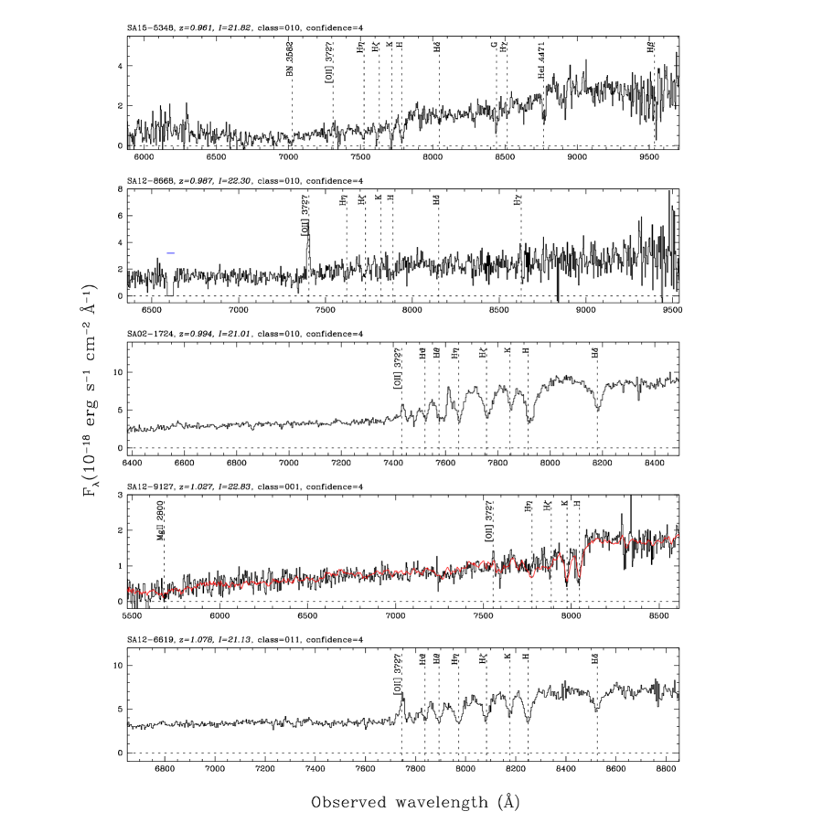
Figure 7: Representative GDDS spectra in the range $0.961<z<1.078$. Galaxies with a range of spectral classifications are shown. The SDSS luminous red galaxy (LRG) composite (shown in red) has been overlaid on the spectrum second from the bottom. The LRG flux $F_{\lambda}$ is binned to $\Delta\lambda=2$ Å rest frame, and rescaled to match the observed spectrum according to the relation $a\times F_{\lambda}+b$ (where $a$ and $b$ are constants). All galaxies shown in this figure and the following four figures have redshift confidence classes of 3 or 4. See the text for further details.

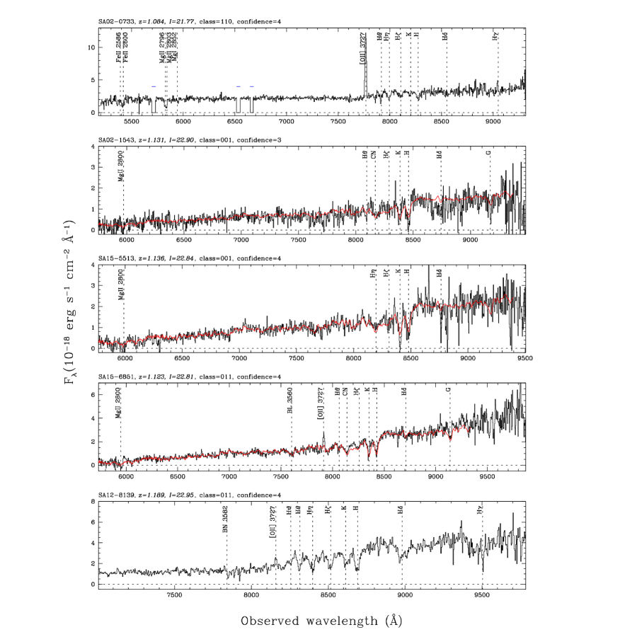
Figure 8: Additional GDDS representative spectra in the range $1.084<z<1.189$. In cases where it is useful for identifying the redshift, the SDSS luminous red galaxy composite is overlain on the spectrum (in red) as in Fig. 7. Masked regions in spectra are indicated using horizontal bars. See the caption of Figure 7 for details.

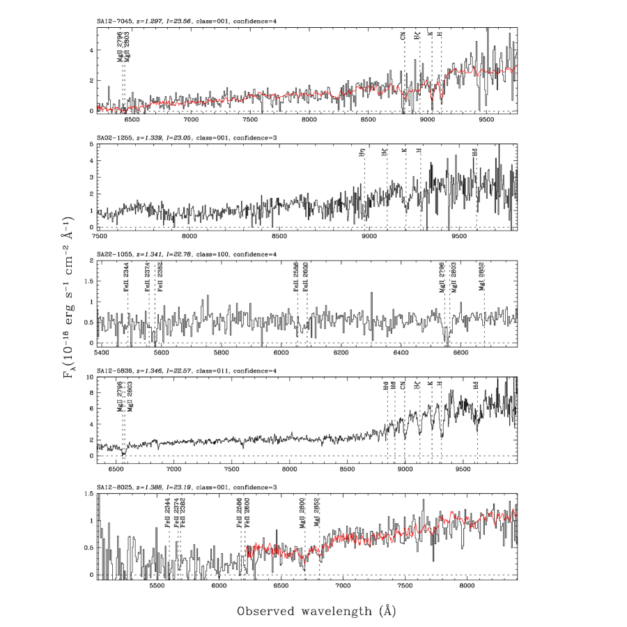
Figure 9: Representative GDDS spectra in the range $1.297<z<1.388$. In cases where it is useful for identifying the redshift, the SDSS luminous red galaxy composite is overlain on the spectrum (in red) as in Fig. 7. Masked regions in spectra are indicated using horizontal bars. See the caption of Figure 7 for details. The spectrum of SA12-7045 and SA12-8025 have been binned to a pixel size of 8 Å.

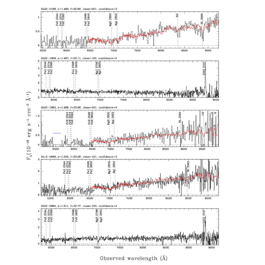
Figure 10: Representative GDDS spectra in the range $1.480<z<1.511$. In cases where it is useful for identifying the redshift, the SDSS luminous red galaxy composite is overlain on the spectrum (in red) as in Fig. 7. Masked regions in spectra are indicated using horizontal bars. See caption of Figure 7 for details. The spectrum of SA22-0189, SA22-1983, and SA12-5869 have been binned to a pixel size of 12, 8, and 7 Å, respectively.

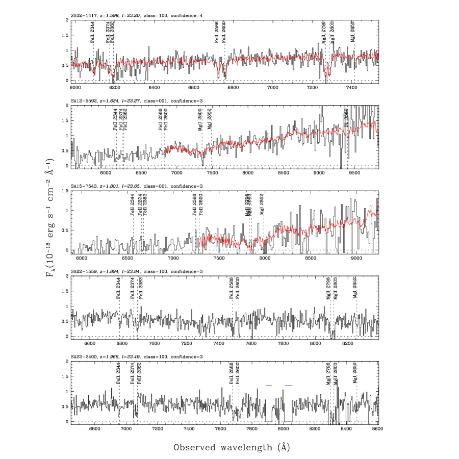
Figure 11: Representative GDDS spectra in the range $1.599<z<1.968$. In the top panel a starburst composite kindly supplied by C. Tremonti is overlaid on the GDDS spectrum. The SDSS luminous red galaxy composite is overlaid on spectra second and third from the top (in red) as in Fig. 7. Masked regions in spectra are indicated using horizontal bars. See caption of Figure 7 for details. The spectrum of SA12-5592 and SA15-7543 have been binned to a pixel size of 12 Å.

All of the multiple 1800s exposures (typically 30–60 spread across multiple nights) making up a mask observation were sky-subtracted (using the shuffled image) and combined into a single 2D frame called the ‘supercombine’. Full details are given in Appendix B. These were then extracted to 1D spectra using standard procedures, but using special software to allow efficient interactive assessment and adjustment (see Appendix C for more details).

3.2 Determination of Redshifts

The absence of artifacts from poor sky subtraction made redshift determination straightforward in the majority of cases. The reality of weak features was also aided by the fact that the iGDDS software used for our analysis (described in Appendix C) provides both one-dimensional and two-dimensional displays of the spectra. An advantage of the Nod and Shuffle technique is that both negative and positive versions of the two-dimensional spectra are recorded and consequently real features display a distinctive pattern that is easily recognized on the two-dimensional spectrum.

The presence of strong emission and absorption features (e.g., [O II]$\lambda 3727$, [O III]$\lambda 5007$, CaII, MgII, D4000, Hydrogren Balmer lines) immediately indicated the approximate redshift in the majority of cases for galaxies at $z<1.2$ At higher redshifts, [OII] can be seen in star-forming objects to $z=1.7$, along with the blue UV continuum and absorption lines (primarily MgII ad FeII). For redder objects, once H&K become undetectable we relied on template matching, which proved to be an excellent aid to redshift estimation. Many such redshifts were obtained using the interactive template manipulation tools built into iGDDS. Good templates covering the 2000-3500Å  wavelength region for a variety of spectral types were not initially available and we eventually constructed some of our own (from galaxies with redshifts that were obvious from other features in their spectra). These templates are shown in Section 5, and proved to be invaluable, particularly for spectra that just exhibit broad absorption features and continuum shape variations in the observed spectral range. On spectra for which the redshifts were uncertain or indeterminate, cross-correlation versus a variety of templates were used to suggest possible redshift/spectral feature matches. These templates included Lyman break galaxies (Shapley et al. 2001), a composite starburst galaxy template (kindly supplied by C. Tremonti), the red galaxy composite from the Sloan Digital Sky Survey published in Eisenstein et al. (2003), and a selection of nearby galaxy spectra obtained from various sources (see Appendix C). Ultimately the most useful templates proved to be the ones constructed iteratively from the GDDS data itself and presented in §5. Since the continuum shape is an important indicator of galaxy redshifts but is not utilized in the cross-correlation technique, all our final redshift determinations were based on a combination of features, not just a cross-correlation peak.

Table 3: Redshift Confidence Classes

Class	Confidence	Note
Failures
0	None	No redshift determined. If a redshift is given in Table 4 it should be taken as an educated guess.
1	$<50$%	Very insecure.
Redshifts Inferred from Multiple Features
2	$>75$%	Reasonably secure. Two or more matching lines/features.
3	95%	Secure. Two or more matching lines/features + supporting continuum.
4	Certain	Unquestionably correct.
Single Line Redshifts
8		Single emission line. Continuum suggests line is [O II]$\lambda 3727$.
9		Single emission line.
AGN Redshifts
1$n$		Class $n$ as above, but with with AGN characteristics

Each object’s redshift was assigned a “confidence class”, based on the system adopted by Lilly et al. (1995) for the Canada-France Redshift Survey. This system is summarized in Table 3. The confidence class reflects the consensus probability (based on a quorum of at least five team members) that the assigned redshift is correct, and takes into consideration each spectrum’s signal-to-noise ratio, number of emission/absorption features, local continuum shape near prominent lines (eg [O II]$\lambda 3727$), and global continuum shape. We did not factor galaxy color into our redshift confidence classifications, which are independent of photometric redshift, although a post-facto inspection shows that the colors of essentially all single emission-line objects (classes 8 and 9) are consistent with the line being [O II]$\lambda 3727$. Redshift measurements for the GDDS sample are presented in Table 4, along with corresponding photometry for each galaxy. Note that in this table non-detections have been placed at the formal 2$\sigma$ detection limits and flagged with an magnitude error of $-9.99$. These detection limits are $B=27.5$ mag, $V=27.5$ mag, $R=27.0$ mag, $I=25.5$ mag, $z=24.5$ mag, $H=21.0$ mag and $K_{s}=21.0$ mag.

3.3 Statistical Completeness

Our analysis of the statistical completeness of the GDDS is broken down into two components. Firstly, there is the component of completeness that quantifies the number of spectra obtained relative to the number of galaxies that could possibly have been targeted. We refer to this component of the completeness as the sampling efficiency of the survey. Secondly there is the fraction of redshifts actually obtained relative to the number of redshifts attempted. We will refer to this as spectroscopic completeness of the survey.

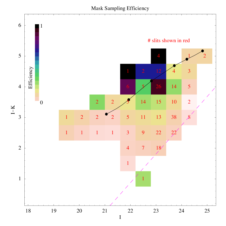
Figure 12: An analysis of sampling efficiency of our GDDS masks. As described in the text, the number counts of faint galaxies at the magnitude limit of the GDDS is much larger than can be targeted on a single multi-object spectroscopic mask. The figure shows a two-dimensional histogram with galaxy counts as a function of magnitude and color. The color of each cell corresponds to the fraction of potential targets in the GDDS images’ field of view actually targeted with a slit. Our algorithm for assigning slits to objects is described in §3 of the text. The dashed line at the bottom-right corner denotes the region in this parameter space below which the $K_{s}$ band magnitudes of galaxies become fainter than the formal 5$\sigma$ $K_{s}=20.6$ magnitude limit of the survey. As described in the text, the bunching up of galaxies in the boxes intersected by this line is mostly artificial, since the counts in these boxes are inflated by blue galaxies undetected in $K_{s}$ that have been placed at the formal detection limit of the survey in our data tables.

The sampling efficiency of the GDDS is investigated in Figure 12. This figure is essentially a visual summary illustrating the success of the mask design algorithm described in §2. The figure shows a two-dimensional histogram quantifying the number of slits assigned to targets as a function of color and magnitude. The sampling efficiency of each cell is keyed to the color bar also shown in the figure. As described earlier, our mask design strategy places heavy emphasis on targeting objects with colors and apparent magnitudes consistent with those of a passively evolving luminous galaxy at $0.8<z<1.8$. Slits were placed on essentially all red galaxies with apparent magnitudes around $I=23.5$ mag (corresponding to the expected brightness of an $M^{\star}$ galaxy at $I\sim 1.3$). The number-weighted average of the sampling efficiency over the cells in the optimal region of this diagram (described §2, and corresponding to $\{22<I<24.5,\ 3<(I-K_{s})<5\}$) is 50%. Thus the GDDS can be thought of as a one-in-two sparse sample of the reddest and most luminous galaxies near the track mapped out by passively evolving high-redshift galaxies in $I$ vs. $I-K$. This sample is augmented by a one-in-seven sparse sample of the remaining galaxy population.

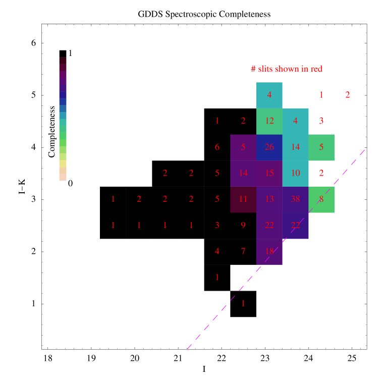
Figure 13: An analysis of spectroscopic completeness in the GDDS fields. This two-dimensional histogram quantifies the success rate in recovering redshifts as a function of color and magnitude. (Note that only those objects with redshift confidence classes of three or higher were considered to be successfully measured). Red numbers embedded in each cell correspond to the number of slits assigned to that portion of the parameter space. The color of the cell denotes the spectroscopic completeness, keyed to the color bar at the top left. The dashed line at the bottom-right corner of the panel denotes the region in this parameter space below which the $K_{s}$ band magnitudes of galaxies become fainter than the formal 5$\sigma$ $K_{s}=20.6$ magnitude limit of the survey. As described in the text, the bunching up of galaxies in the boxes intersected by this line is mostly artificial, since the counts in these boxes are inflated by blue galaxies undetected in $K_{s}$ that have been placed at the formal detection limit of the survey in our data tables.

Our success in translating slits into redshifts is shown in Figure 13. This diagram is the close analog to the previous figure, with the difference being that cell colors are keyed to spectroscopic completeness instead of sampling efficiency. Spectroscopic completeness is calculated simply by dividing the number of high-confidence redshifts (confidence class greater than or equal to 3) in each cell by the number of slits assigned in the same cell. As expected, spectroscopic completeness is a strong function of apparent magnitude. Spectroscopic completeness is 100% brighter than $I=22$ mag, dropping to around 50% at $24.0<I<24.5$ mag (11 redshifts out of 20 attempted).

The overall spectroscopic completeness of the GDDS depends on the minimum value of the redshift confidence that is considered acceptable. Slits were placed on 317 objects. Three of these slits contained two objects and thus redshift determinations were attempted for 320 objects. Of these, approximately 3% (11 objects) were so badly compromised by overlap or contamination that they were judged to be invalid. Of the 309 valid spectra, approximately 79% of the attempts resulted in moderately high confidence (classes 2 and 9) or very high confidence (classes 3,4, and 8) redshifts. As will be shown in §4, the great majority of these were in our target redshift range, with only a very modest contamination by very low redshift objects. (Twelve objects were found to be late-type galactic stars, and 5 objects were found to be $z\sim 0.1$ extragalactic HII regions). An additional 10% of GDDS targets had very low confidence redshifts assigned (class 1 and 0). The remaining 11% of targets had no redshifts assigned.

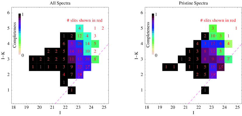
Figure 14: An analysis of the relative completeness for our full sample (shown at left), and a subsample constructed from only those spectra unaffected by spectrum overlaps (shown at right). The dashed line corresponds to the completeness limit of the survey.

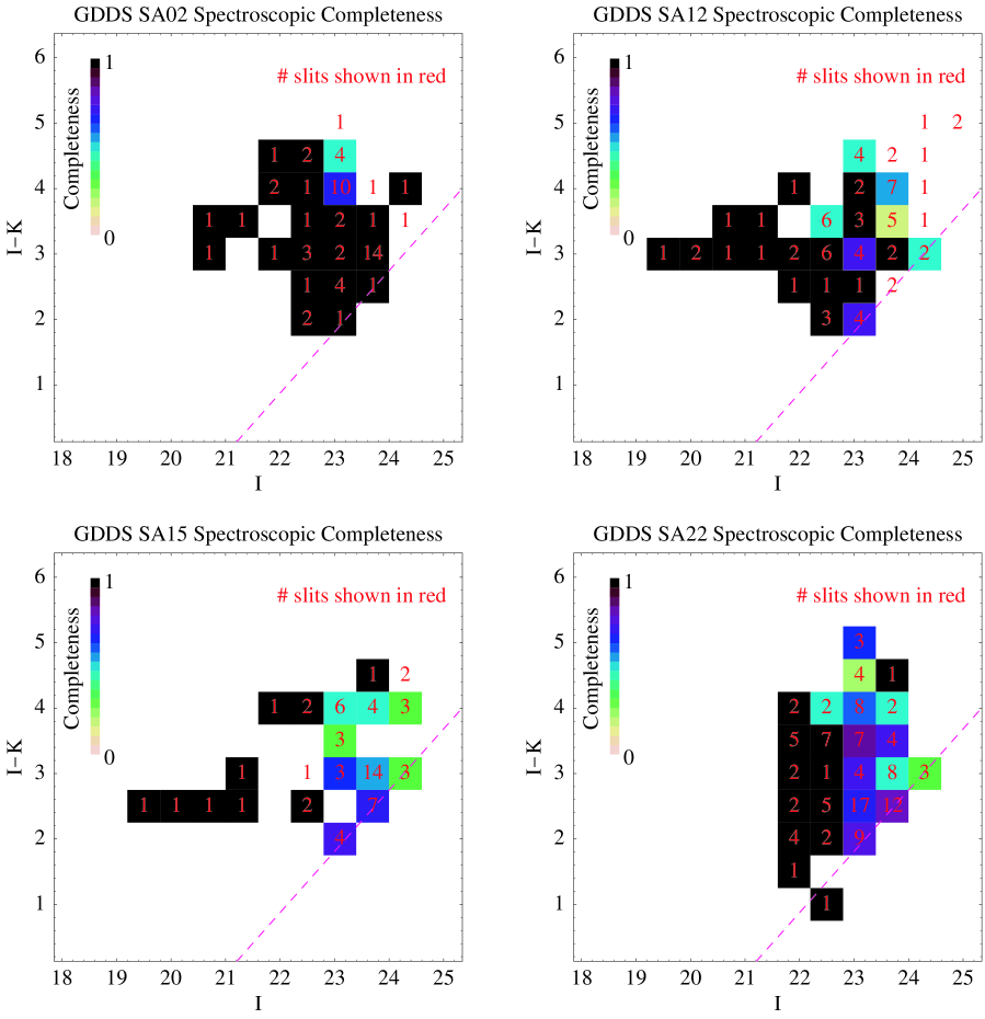
Figure 15: An analysis of the field-to-field variation in the spectroscopic completeness in the GDDS. Two-dimensional completeness histograms for GDDS-SA02 (top-left), GDDS-SA12 (top-right), GDDS-SA15 (lower-left), and GDDS-SA22 (lower-right) are shown. As for all similar figures in this paper, the dashed line at the bottom-right of the figure denotes the region of color-magnitude space below which measured $K_{s}$ photometry drops below the formal magnitude limit of the survey. See the caption to the previous figure for additional details.

It is interesting to consider the main sources of spectroscopic incompleteness in the GDDS. The obvious gradient in incompleteness as a function of apparent magnitude seen in Figure 13 indicates that the main cause of incompleteness is photon starvation, particularly for red systems with little rest-UV flux. However, in some cases we were unable to obtain redshifts for relatively bright systems on account of overlapping spectral orders. Our mask design strategy was a trade-off between maximizing the number of objects we attempted to get redshifts for, and minimizing spectrum order overlaps. It is worthwhile to try to quantify the relative importance of these competing effects. An attempt at doing this is illustrated in Figure 14, which shows a comparison between the cell-to-cell completeness in our full sample and the corresponding cell-to-cell completeness in a sub-sample of “pristine” objects unaffected by spectrum overlaps. Note that the spectroscopic completeness of our red galaxy sample is nearly unchanged in both panels of this figure, while greater variation is seen in the blue population. As described in §2, our mask-design strategy was optimized for red galaxies, and a particular effort was made to avoid spectrum overlaps in this population in order to preserve continuum shape. On the other hand, our emphasis in laying down slits on blue galaxies was to use the detector area efficiently even at the expense of sometimes allowing spectrum overlaps to occur (since emission line redshifts can often be determined from these by studying the two-dimensional spectra). We therefore expected to see a somewhat greater variation in the cell-to-cell completeness of blue galaxies as a function of slit overlap class, and Figure 14 is consistent with this.

We also note that the extra freedom used when assigning slits to blue galaxies results in substantially greater field-to-field variation in the spectroscopic completeness of blue galaxies in the GDDS. The field-to-field completeness of the GDDS is shown in Figure 15. Significant variations in the total completeness in each field are seen, ranging from a high of 87% in GDDS-SA02, to a low of 60% in GDDS-SA12. It is important to note that most of this field-to-field variation is in the blue population, and the cell-to-cell completeness near the red galaxy locus of the color-magnitude diagram in each panel of this figure remains quite stable.

3.4 Spectral Type Classification

In addition to the redshift confidence class, each object was assigned a series of spectral classifications that record both the features that were used to determine the redshift and a subjective classification of the galaxy’s spectral type. Our spectral classifications are presented in Table 5. The first column notes whether any features indicative of AGN activity are seen in the spectrum (0 = no, 1 = yes). The next 11 entries specify the presence (1) or lack (0) of the most common spectral features used in the redshift determinations. A (2) in any of these columns indicates that the particular feature did not fall within the wavelength range of our spectra. In some cases the spectral range covered by a particulary object was reduced by overlap or contamination from other objects. The “template” column in Table 5 identifies those objects whose redshifts were based largely on a match to a template spectrum, either a composite from our own spectra (see below) or an external spectrum. It is emphasized that spectra on different masks had different exposure times, and order overlaps impacted some spectra more than others, so these feature visibility classifications should be used as a general guideline only and not over-interpreted.

The last column in Table 5 lists the spectral class assigned to each object. This classification is based on three digits that flag young, intermediate age, and old stellar populations. Objects showing pure, or nearly pure, signatures of an evolved stellar population (e.g. D4000, H&K, or template matches) are assigned a class of “001”. Objects that are dominated by the flat-UV continuum and strong emission-lines characteristic of star forming systems are assigned a “100” classification, those showing signatures of intermediate ages (e.g. strong Balmer absorption) are assigned a class of “010”. Many objects show characteristics of more than one type and so are assigned classes that are the composite of old (001), intermediates (010) and young (100) populations. Objects listed as “101” may show strong H&K absorption and 4000Å  breaks and yet have a flat-UV continuum tail indicative of a low-level of ongoing star formation.

4 SUMMARY OF REDSHIFTS AND SPECTRAL CLASSIFICATIONS

A graphical synopsis of the spectroscopic information in the GDDS is presented in Figure 16, which shows the number vs. redshift histogram for our sample, color-coded both by confidence class and by spectral class. The shading of the box shows the confidence class, the color of the label reflects the spectral class. A number of interesting aspects of our experiment are evident in Figure 16. Firstly, despite our use of four widely separated fields, we remain significantly impacted by large-scale structure and sample variance. The factor of two deficit of objects at $z=1.2$ cannot be the sign of failure to recognize objects at this redshift as we do considerably better at $z=1.3$, a more difficult redshift. Secondly, it is clear that our success rate drops steeply at $z>1.5$, where our fraction of high confidence redshifts drops from $>90$% to $\sim 30$%. As described in §3.3, this is mostly because these objects, and the red ones in particular, are fainter than the average galaxy in the sample, particularly at wavelengths shortward of the $I$-band used to set the magnitude limit of the sample.

The following summarizes the fractions of different stellar populations amongst objects with high-confidence redshifts in the GDDS. Approximately 15% of the objects observed showed spectra with pure old stellar populations (class 001). The fraction with strong signatures of evolved stars (i.e. objects with classes 001 or 011) is 22%. Galaxies showing some evidence for intermediate age stellar population features (classes 110, 010, 001) accounted for 46% of the sample. About 25% of galaxies had pure intermediate age populations (class 010), and 24% of the sample appear to be dominated by young populations (class 100). We were unable to assign any spectral classifications to 10% of objects with high confidence redshifts.

The fraction of galaxies with evidence of old populations peaks at $z\sim 1$ and falls off steeply at higher redshifts. Some of this reflects the increasing impact of the non-$K_{s}$-detected objects that were added to the sample on the basis of their photometric redshifts. A number of the $z>1.5$ objects, however, do have $K<20.6$ and some of these have red $I-K_{s}$ colors and yet still show essentially flat UV spectra dominated by massive stars. This is not surprising given the shape of the $V-I$ vs. $I-H$ (or $I-K_{s}$) two-color diagram (McCarthy et al. 2001). At $z>1.5$ the bulk of the red $I-K_{s}$ population has blue $V-I$ colors. The spectroscopic properties of these galaxies, along with inferred ages from stellar population synthesis models, will be presented in a companion paper (McCarthy et al. 2004, in preparation).

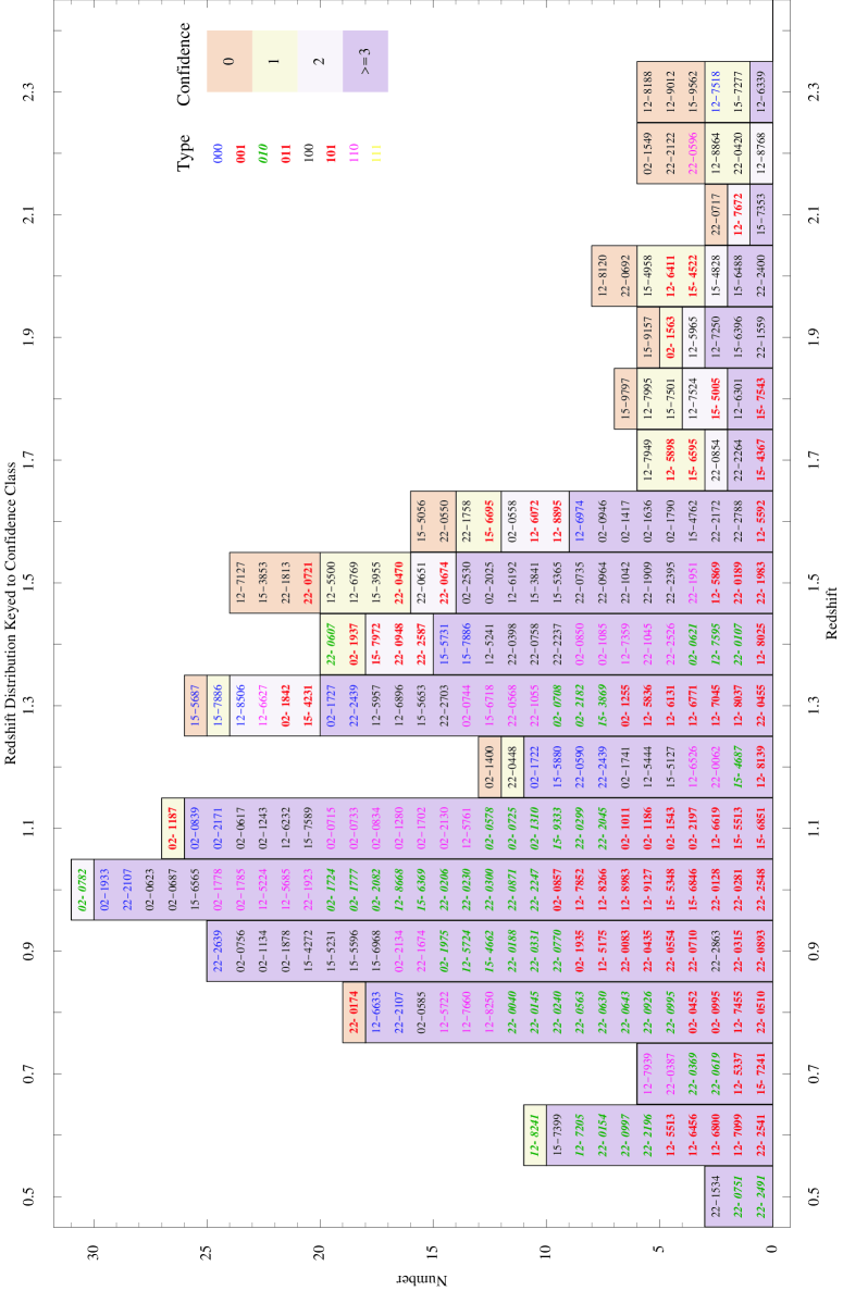
Figure 16: Master summary of the GDDS. This histogram illustrates the redshift distribution of our sample as a function of confidence class and spectral type. Bar colors indicate confidence in the redshifts, keyed to the system defined in Table 2. Individual objects are labeled in each histogram and sorted by spectral class. Label colors are keyed to spectral class.

5 COMPOSITE TEMPLATE SPECTRA

As described earlier, redshifts were determined by visual examination of the spectra, comparing with spectral templates and looking for expected redshifted emission and absorption features. The most uncertain aspect at the start of our survey was the appearance of normal galaxies in the 2000–3000Å region. Early-type quiescent galaxy spectra are expected to be dominated by multiple broad absorption features in this region (for example see the mid-UV spectra of elliptical galaxies in Lotz et al. 2000) which come primarily from F & G main sequence stars (Nolan, Dunlop & Jimenez 2001). In contrast late-type actively star-forming galaxies should have a featureless blue continuum with narrow ISM absorption lines superimposed (for example see the HST starburst spectra in Tremonti et al. 2003).

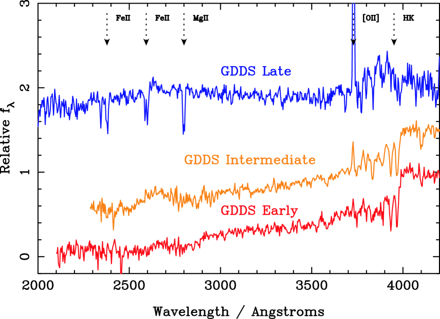
Figure 17: The three GDDS template composite spectra used for redshift comparison. These were constructed internally from our sample from galaxies covering a range $0.6<z<2$ with high confidence redshifts. The templates are plotted at 3.5Å per pixel resolution and are normalized to unity at 4200Å, they are offset vertically in the plot for clarity. Some of the more common features are marked. Only the UV portion of the templates is shown.

For the first two GDDS fields we primarily used the Luminous Red Galaxy template of Eisenstein et al. (2003) and spectra of the $z\sim 1.4$ radio galaxies 53W091 (Spinrad et al., 1997) and 53W069 (Dunlop 1999) for our early-type reference templates. For late types we used a composite spectrum made from an average of the local starburst galaxy starforming regions of Tremonti et al. After we had reduced our first two fields and obtained preliminary redshifts we then constructed our own templates by combining GDDS spectra. We had three principal motivations for doing this. The first was to obtain a better match in spectral resolution; the second was to improve the UV coverage especially in the early-type template and the third was to make templates corresponding to galaxies in an earlier evolutionary epoch in the history of the Universe.

In order to make the templates we visually identified similar looking spectra with confidence level 3 or 4 redshifts. The full redshift range of GDDS $0.6<z<2$ was used in order to produce templates with a wide range of spectral coverage. Of course this large redshift range is less than ideal because on average the resulting UV portion of the templates will come from higher redshift objects than the optical portion. However we decided that since the primary use of these templates were for redshift matching, the wider wavelength coverage would be of greater importance. It remains true that the UV portion of the templates ($\lambda<3000$Å) comes mostly from $z>1$ objects and this was where our previous set of templates were most inadequate. We emphasize that these redshift templates are different from the composite spectrum analyzed by Savaglio et al. (2004), where it is more important to have a more restricted redshift range.

The template construction process fully allowed for masking and disparate wavelength coverage in the different spectra. Given a set of input spectra the construction process was as follows. Firstly one spectrum (typically at the median redshift) was chosen as a master for the purposes of normalization. Next all the other templates were scaled to the same normalization as the master by computing the average flux in the non-masked overlapping regions. Finally a masked average was performed of all the normalized templates (the mask being either 1 or 0 depending on whether a given spectrum included that part of the wavelength region with good data).

For the early type template we combined 8 convincing early type spectra with redshifts $0.6<z<1.5$ and for the late type template we combined 23 late type spectra with $0.8<z<2.0$. We also found it desirable to make an intermediate type template (i.e., somewhat red but with signs of star-formation such as [OII] emission) as these were especially poorly represented in our first template set. For this we used 8 galaxies with $0.7<z<1.3$. The resulting three templates are plotted in Figure 17.

6 CONCLUSIONS

The Gemini Deep Deep Survey was undertaken in order to explore galaxy evolution near the peak epoch of galaxy building. The survey probes a color-selected sample in a manner that minimizes the strong star-formation rate selection biases inherent in most high-redshift galaxy surveys. It is designed to bridge the gap between landmark surveys of highly complete samples at $z<1$ (Cowie et al. 1994; Lilly et al. 1995; Ellis et al. 1996) and UV-selected surveys at higher redshift (Steidel et al. 1996; Shapley et al. 2001; Steidel et al. 2003). The signal-to-noise ratios of the spectra in the GDDS are sufficient to distinguish old stellar populations (dominated by F-type stars) from post-starburst systems (dominated by A-type stars) and reddened starbursts with their flat spectra and strong interstellar lines. In this paper we have described the motivation for the survey, the choice of fields, the experimental design underlying our choice of targets, and our data reduction process. We have presented final catalogs of redshifts and photometry and an analysis of their statistical completeness. Spectra for individual objects are available as an electronic supplement to this paper. Further information on the GDDS and the data reduction software used in the project are available on the World Wide Web at http://www.ociw.edu/lcirs/gdds.html.

Acknowledgments

This paper is based on observations obtained at the Gemini Observatory, which is operated by the Association of Universities for Research in Astronomy, Inc., under a cooperative agreement with the NSF on behalf of the Gemini partnership: the National Science Foundation (United States), the Particle Physics and Astronomy Research Council (United Kingdom), the National Research Council (Canada), CONICYT (Chile), the Australian Research Council (Australia), CNPq (Brazil) and CONICET (Argentina)

The Gemini Deep Deep survey is the product of a university/institutional partnership and would not have been possible without the work of many people. We thank Matt Mountain, Jean-René Roy and Doug Simons at the Gemini Observatory for their vision in supporting this project in the midst of many other observatory priorities, and for the time, energy and manpower they have invested in the making Nod & Shuffle a reality on Gemini. It is a pleasure to thank Matthieu Bec and Tatiana Paz at the Gemini Observatory for their work in implementing the modifications to the GMOS telescope control system and sequence executor needed in order to support the Nod & Shuffle mode. We are grateful to the entire staff of the Gemini Observatory for undertaking the queue observing for this project in such an efficient manner, and for the kind hospitality shown to us during our visits.

We also thank the Instrumentation Group at the Herzberg Institute of Astrophysics for working with us and with Gemini in order to help make GMOS Nod & Shuffle a reality. Many members of the HIA Instrumentation Group went beyond the call of duty in support of this project, but we would like to particularly thank Bob Wooff and Brian Leckie at HIA for their quick response and willingness to work late into the night during a weekend to fix some early problems we encountered, which saved us from losing a night of observing during the science verification phase of the GDDS. We also thank Richard Wolff at NOAO for doing much of the microcode programming needed for this project.

RGA and RGC acknowledge generous support from the Natural Sciences and Engineering Research Council of Canada, and RGA thanks the Government of Ontario for funding provided from a Premier’s Research Excellence Award. KG & SS acknowledge generous funding from the David and Lucille Packard Foundation. H.-W.C. acknowledges support by NASA through a Hubble Fellowship grant HF-01147.01A from the Space Telescope Science Institute, which is operated by the Association of Universities for Research in Astronomy, Incorporated, under NASA contract NAS5-26555.

Appendices

Appendix A NOD & SHUFFLE OBSERVATIONS WITH GMOS

The principles of the Nod & Shuffle technique are described in Glazebrook & Bland-Hawthorn (2001). The basic ideas behind the mode are very similar to those of the Va et Vient strategy for sky subtraction (Cuillandre et al. 1994; Bland-Hawthorn 1995). Our specific Nod & Shuffle configuration is shown schematically in Figure 18, and corresponds to the ‘Case 1’ strategy shown in Figure 2(a) of Abraham et al. (2003). Slits were 0.75 arcsec wide (giving a spectral FWHM of $\simeq 17$Å) and were designed to take advantage of the queue observing mode of the telescope by being optimized for seeing $<0.85$ arcsec. In this seeing the target galaxies were mostly unresolved. In Nod & Shuffle mode the telescope is nodded between two positions along the slit denoted ‘A’ and ‘B’, as shown in Figure 18. For our first mask observations on the 22^h field we used a 2.0 arcsec long slit, since the nod distance was 1.0 arcsec the targets appear on the slit in both A and B positions ($\pm 0.5$ arcsec from the slit center). The shuffle distance was 28 pixels which produces a shuffled B image immediately below the A image with a small one pixel gap. For subsequent fields we increased the slit length to 2.2 arcsec and the shuffle to 30 pixels as analysis of the first field convinced us that a slightly longer slit would be beneficial to reduce the impact of the ‘red end correction’ issue described below.

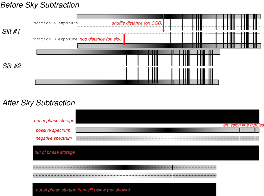
Figure 18: Schematic of the Nod and Shuffle mode used in the GDDS. When the telescope is in the object position, CCD area ‘A’ records a spectrum. The ‘sky’ position records the nodded spectrum (in this case the telescope has been nodded 1.0 arcsec along the slit direction). The area ‘B’ is unilluminated by the mask and serves as a storage area for the sky position. The image difference A$-$B subtracts the sky, and leaves a positive and negative object spectrum for subsequent extraction.

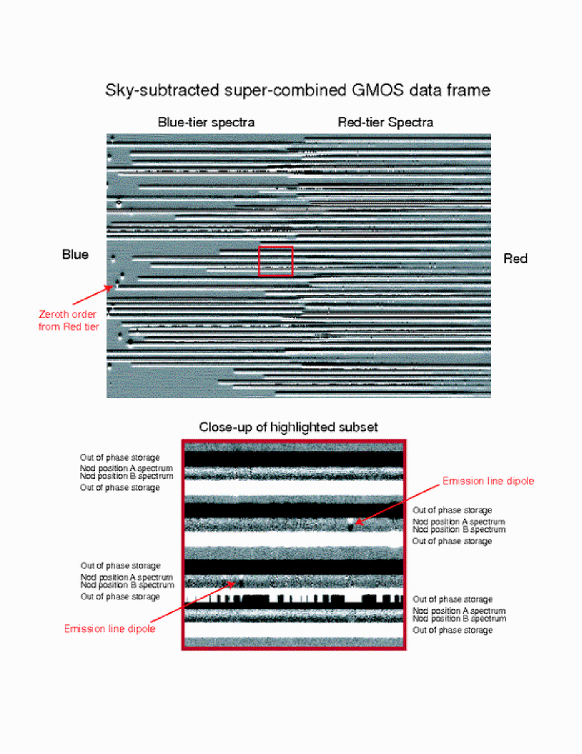
Figure 19: An image showing a sky-subtracted “supercombined” frame for the GDDS-SA22 field. Object spectra are sandwiched between positive and negative sky spectra on the mask. The lower half of the figure shows a magnified view of the small rectangular region near the center of the mask image. This magnified view shows subsets of four spectra with characteristic positive and negative continua and emission lines. Note that for clarity we have reversed the GMOS data format to show bluer wavelengths to the left.

At each A and B position we observed for a 60 sec exposure before closing the shutter and nodding the telescope and shuffling the CCD. Our standard GDDS exposure consisted of 15 cycles with A$=$60s and B$=$60s (i.e. a total of 1800s open shutter time on target before reading out). There is of course extra overhead associated primarily with moving the telescope and guide probes, for the GDDS observing setup this typically added 25% to the total observing time. We found that this Nod & Shuffle setup gave a sky-residual of only 0.05–0.1%, which is well below the Poisson limit for our stacked exposures, except for the brightest few night sky lines. The reader is referred to Abraham et al. (2003) and Murowinski et al 2004 (in preparation) for a more detailed description of the implementation, observing sequence and sky-subtraction performance of Nod & Shuffle mode on GMOS.

A typical mask observation consisted of approximately 50 half-hour exposures observed across many nights. In order to fill in the gaps between CCD chips the grating angle was changed between different groups of observations in order to dither the MOS image along the dispersion ‘X’ axis relative to the CCD. Approximately one third of the data was taken with a central wavelength of 7380Å, one third with 7500Å and the final third with 7620Å. The CCD gaps were filled in when the different positions were combined to make a master frame.

Similarly it is also desirable to dither in the orthogonal, ‘Y’ direction, i.e. parallel to the spatial axis, in order to minimize the effects of shallow charge traps aligned with the silicon lattice of the CCD. These charge traps manifest themselves in the shuffled images as short pairs of streaks in the horizontal, or dispersion, direction. Each pair is always separated by the shuffle distance. We speculate these charge traps originate from subtle detector defects that are repeatedly pumped by the shuffle-and-pause action. Since the traps always appear at the same place on the CCD, their undesired effect can be greatly reduced by dithering the image along the Y axis and rejecting outliers during stacking. To accomplish this dithering the CCD was physically moved using the Detector Translation Assembly (DTA). During normal GMOS operation, this stage is used to actively compensate for flexure in the GMOS optical chain during exposures. Additional offsets can be applied between exposures in order to position the image on different pixels on the array.

Our standard observing block thus consisted of the following six-step sequence:

1. The grating was set to one of the 3 positions used (e.g. 7500Å). The DTA was homed.

2. An 1800s exposure was recorded using Nod & Shuffle (A$=$60s, B$=$60s, $\times$ 15 cycles).

3. An 1800s exposure was recorded with the DTA offset by +41µm  (+3 pixels) along the spatial axis.

4. An 1800s exposure was recorded with the DTA offset by +81µm  (+6 pixels) along the spatial axis.

5. An 1800s exposure was recorded with the DTA offset by $-$41µm  ($-$3 pixels) along the spatial axis.

6. An 1800s exposure was recorded with the DTA offset by $-$81µm  ($-$6 pixels) along the spatial axis.

This same sequence would then be repeated for the next grating position, and this pattern of changing the central wavelength and taking a sequence of 5 exposures was repeated until the required number of exposures was completed. In practice not every sequence had this exact number of steps and sequence due to observing constraints, but an approximate balance was maintained among the different DTA offset positions which was all that was required for the stacking of the data.

Appendix B REDUCTION OF TWO-DIMENSIONAL DATA

The goal of the 2D reduction was to combine all the individual 2D dispersed 1800s exposures for each mask with outlier rejection to make a master ‘supercombine’ 2D sky-subtracted dispersed image. This is then used for the next stage — extraction to 1D spectra. The GDDS 2D data was reduced using IRAF and the Gemini IRAF package, in particular the v1.4 GMOS sub-package. To handle the peculiarities of Nod & Shuffle data two new software tasks (gnsskysub and gnscombine) were written by us. These have now been incorporated into the standard IRAF GMOS package distributed by the Gemini Observatory.

The first step in the 2D data reduction was to bias subtract the individual runs using a master bias frame (the average of typically 20 bias frames taken during the observing period). GMOS exhibits 2D bias structure so a 2D bias subtraction is done with the gireduce task.

The next step was to sky-subtract all the runs using the gnsskysub task. This simply takes the frame, shifts it in Y by the shuffle step, as recorded in the image header, and subtracts it from itself. This results in clean sky-subtracted spectra sandwiched between regions of artifacts, as shown in Figure 18. These subtracted frames are then visually examined to make a list of relative dither offsets. In most cases these are as given by the nominal DTA offsets, with occasional 1–2 additional pixel shifts between different GMOS nights (these shifts are then recovered by sky-line fitting and cross-correlation). In some cases the objects moved slightly in the slits relative to their nominal position due to an error in setting the tracking wavelength in the telescope control system. In order to handle these extra offsets actual emission lines in bright galaxies were centroided in X and Y and used to define the offsets. Calculating the offsets directly relative to the object positions in this way results in some fuzziness of slit edges in the 2D combined frames, but since the inter-slit offsets were only a few pixels and only a few frames were affected, this did not turn out to be a serious problem in practice. The final result of the inspection is a list of X,Y offsets between the objects in different dispersed images.

Once the offsets are known image combination proceeds with the gnscombine task which generates sky-subtracted frames using gnsskysub and combines them using a variance map calculated from the median count level in the non-subtracted frames and the known readout noise and Poisson statistics. Outliers (cosmic rays and charge traps) are rejected using a 7$\sigma$ cut and retained data is averaged. The outlier rejection was checked visually by comparing frames combined with and without rejection and it was verified that only genuine outliers were rejected. A median 2D sky frame is also produced which is used for later wavelength calibration and further noise estimates.

We first combined the frames in 3 groups according to the central wavelength using gnscombine, i.e. a combined frame was produced for each of the 7380Å, 7500Å  and 7620Å positions. At this point the combined frames are a single Multi-Extension FITS (MEF) file where each extension represents a separate GMOS CCD as a 2D image. The next step is to use the gmosaic task to assemble the three images for each group into a single contiguous image using the known geometric relationship between the three CCDs. gmosaic was used in the mode where the assembly was done to the nearest pixel; no re-sampling or interpolation scheme was used in order to preserve pixel independence in the noise map. Since the data is 4$\times$ over-sampled this does not result in any significant degradation. Inspection of the gmosaic’d images showed the spectral continuity across the CCD gaps was good to $\pm 1$ pixel and subsequent wavelength calibration showed the positioning in the dispersion direction was of a similar accuracy.

Finally the three gmosaic’d combined frames for the 7380Å, 7500Å  and 7620Å positions were mosaiced again into the final ‘supercombine’ frame. The task gemcombine was used to accomplish this with offsets calculated from fitting to sky lines. A binary mask denoting the position of CCD gaps and bad columns was also used to remove these features from the final supercombine by replacing them with real data from the other frames.

The final products of this process are: (a) a supercombined (i.e. sky subtracted) frame corresponding to the the stack of all the 2D data — an example is shown in Figure 19; (b) a corresponding supercombined sky frame showing the emission from the night sky. It should be noted that no attempt was made to flat-field the data. This is not required to get accurate sky-subtraction with Nod & Shuffle. The effect of pixel-pixel variations in the final object spectra are greatly reduced by the extensive dithering in any case. Some residual flat-field features, primarily fringes, are visible in the brightest spectra at the few percent level, but these do not seriously impact our faint spectra.

Appendix C EXTRACTION OF ONE-DIMENSIONAL SPECTRA

One-dimensional spectra were extracted from the two-dimensional stacked image frames using iGDDS, a publicly available spectral extraction and analysis program for Mac OS X that we have written for use with Nod & Shuffled GMOS data. iGDDS operates in a manner that is rather different from the familiar command-line driven tools used by astronomers (e.g. IRAF, FIGARO, MIDAS, etc.), and it is intended to be highly interactive and take full advantage of the graphical capabilities of modern computers. The program functions as an electronic catalog with interactive tools for spectral aperture tracing, one-dimensional spectrum extraction, wavelength calibration, spectral template fitting, and redshift estimation. All these tools are linked. For example, selecting an object in a catalog displays its two-dimensional image and corresponding aperture trace. This aperture trace can be reshaped by dragging with a mouse, resulting in a newly extracted one-dimensional spectrum. Clicking the mouse on a feature on this spectrum immediately displays this feature on a corresponding two-dimensional image. This feature can then be selected and a trial redshift assigned, which results in the superposition of a comparison template spectrum on the object spectrum. The template can then be dragged with the mouse to refine the redshift or try other possibilities.

All analysis steps for all spectra on a GMOS mask are stored in a single document file which can be shared with colleagues and interactively modified. The saved iGDDS document files used by our team are publicly available, and the interested reader may find these to be a useful starting point for further exploration of the GDDS data set.

C.1 Aperture Tracing

Spectra were extracted from the supercombined stack using aperture traces defined by a fourth-order bezier curve. Positive and negative apertures (corresponding to the A and B nod and shuffled positions) were defined relative to this curve. The sizes of these apertures and the distance between them were allowed to vary independently. (As described in §C.4, in some cases it is useful to discard a single A or B position channel in order to avoid contamination from overlapping spectra). In most cases the spectra were sufficiently bright to allow a well-defined trace to be determined visually (after lightly smoothing the two-dimensional image and displaying the galaxy spectrum with a large contrast stretch). However, the very faintest galaxies in our sample proved too dim to allow a reliable trace to be estimated, and for these objects simple horizontal trace was used.

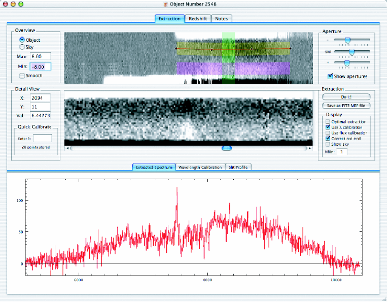
Figure 20: An example showing an extraction window in iGDDS for object 2548 in the $22^{\rm h}$ GDDS field. Two sub-images and the corresponding one-dimensional spectrum are shown. The top sub-image shows a compressed view of a horizontal slice (34 pixels high and 4608 pixels wide) across the supercombined 2D image at the $y$-coordinate of the slit. The bezier curve defining the trace for the spectrum is shown as the solid red line in the top sub-image. Control points for the curve are shown as black circles attached to the endpoints of the curve. Dragging a control point with the mouse changes the shape of the trace. The transparent yellow and purple regions linked to the trace correspond to the negative and positive extraction apertures. The transparent green rectangle in the top sub-image shows the portion of this image that is magnified for detailed inspection in the lower sub-image. The extracted spectrum for this object is shown at the bottom of the window. Note that at this stage in the extraction the spectrum is not fluxed.

A screenshot from iGDDS illustrating the aperture tracing process is shown in Figure 20. In this figure the top sub-image shows a compressed view of a horizontal slice across the supercombined 2D image at the $y$-coordinate of the slit (34 pixels high and 4608 pixels wide). The fourth-order bezier curve defining the trace for an individual spectrum is shown as the solid red line in the top window. The transparent yellow and purple regions on this image are linked to the trace and correspond to the negative and positive apertures used to extract the one-dimensional spectrum.

C.2 Linear and Optimal Extraction

One-dimensional spectra were extracted from the supercombined images using both linear and optimal extraction procedures. Both sets of extractions are available in the public data release of the GDDS observations described in §C.5 below.

Our optimal extractions were constructed using profile weights defined by projecting the spectra in the spatial direction following the bezier curves which define their traces. This procedure resulted in smooth extraction profiles that resembled gaussians for most galaxies, although in cases where spectrum overlaps occurred (described in greater detail §C.4) the resulting weight profiles were spuriously asymmetric. The optimal extractions should not be trusted for these objects. We therefore recommend that those readers interested in making uniform comparisons between all spectra in the GDDS use only the linearly extracted spectra. Optimally extracted spectra can be trusted for those objects with recorded spectrum overlap classifications of zero in Table 3, and these do have slightly improved signal-to-noise relative to their linearly extracted counterparts. However, the signal-to-noise improvement is modest (of order 5%) on account of the narrow slit lengths in the GDDS masks. For the sake of consistency, only linearly extracted spectra have been shown in the figures throughout the present paper.

Small artifacts on the two-dimensional supercombined images were masked out using iGDDS prior to extraction. Our masking procedure works by excluding aberrant pixels from the resulting average over the spatial direction in a given column. The procedure is clearly of rather limited usefulness, and was only adopted in those cases where at most a few pixels in a given column were contaminated by artifacts. In cases of more severe contamination, we chose to eliminate the column completely (leaving gaps in the spectrum) rather than to patch over the bad data. As will be described in §C.5, the output data format for the GDDS spectra retains a record of which wavelength points on a spectrum have been patched.

Including the effects of bad pixel masking, extraction proceeded as follows. Consider a single column in a two-dimensional spectrum containing $n$ rows. Denote the flux in the $i$th pixel by $F_{i}$, its variance by $\sigma_{i}^{2}$, and let the discrete variable $\mathcal{M}_{i}\in\{-1,0,1\}$ take on the value $1$ in the case that the pixel is in aperture A, $-1$ in the case that the pixel is in aperture B, and $0$ in the case that the pixel is masked. Assuming $n_{A}$ pixels are contained within apertures A and B, a simple estimator of the total flux in the case of linear extraction with masked regions is:

$$F=n_{A}\cdot{\sum_{i=1}^{n}(\mathcal{M}_{i}/\sigma_{i}^{2})F_{i}\over\sum_{i=1}^{n}|(\mathcal{M}_{i}/\sigma_{i}^{2})|}$$ (C1)

In other words, the flux is now the average over the non-rejected pixels multiplied by the total number of masked and un-masked pixels in both apertures.

The corresponding case for optimal extraction is only slightly more complicated. Denoting the optimal extraction profile by a continuous variable $P_{i}\in\{0..1\}$ (with $P_{i}\equiv 0$ for pixels in the column outside the aperture), it is straightforward to show that the maximum likelihood estimator for the true total flux is given by:

$$F=\sum_{i=1}^{n}P_{i}\cdot{\sum_{i=1}^{n}P_{i}(\mathcal{M}_{i}/\sigma_{i}^{2})F_{i}\over\sum_{i=1}^{n}P_{i}^{2}|(\mathcal{M}_{i}/\sigma_{i}^{2})|}$$ (C2)

Note that if we set $P_{i}=1$ then we recover the linear extraction case.

C.3 Flux Calibration, Atmospheric Absorption Correction, and Red Fix Correction

Since precise flux calibration is impossible for observations accumulated over many nights (spread over months in some cases) under varying conditions, the flux calibration was carried out using observations of standard stars obtained as part of the GMOS queue baseline calibration. These data were reduced using the standard routines in IRAF and calibrations deduced for each field. A mean aperture correction of a factor of 3.5 was applied to each spectrum. In the end, the calibrations were so similar from field to field that the same one was used for all. For most objects the relative flux calibration appears to be quite good, as evidenced by the fact that composites made from these spectra agree extremely well with composites from other surveys, e.g., the SDSS luminous red composite of Eisenstein et al. (2003). However, the absolute flux for an individual object may be in considerable error (we think they should only be trusted to within about a factor of two), since no attempt was made to allow for overlapping spectra, masked regions, flat-fielding of 2D spectra, etc. We therefore caution that the fluxes are relative only.

As the 1D spectra were initially being extracted from the 2D spectra, it almost immediately became apparent that there was a problem in that the continua became too low or even negative at the extreme red end of the wavelength region. Since one expects that the nod and shuffle technique would result in perfect sky subtraction, this was initially very puzzling. On further examination it became evident that the strong sky lines displayed “tails” so that there was spatial extension of the lines that increased in strength with wavelength. Unfortunately, in the nod and shuffle technique, the protrusion of these on either side of the spectra means that they are superimposed and subtracted from the object spectrum during the shift-and-combine operation. The origin of this effect is charge diffusion in the silicon which is a strong function of wavelength and it has only become apparent since we are attempting to extract extremely faint target spectra that are stored immediately adjacent to extremely strong sky spectra on the CCD. The effect could be reduced or avoided by increasing the distance between the object and sky or the two object positions in our case, at the cost of less efficient use of the detector area. For any given mask design, the magnitude of the effect depends on the precise relative position of the object in the slitlet but, in our case, the only practical way to correct for it was to establish an average correction for all objects in a mask and then apply that to all spectra.

A correction curve to account for this effect was derived empirically for each mask. First, the variation of the strength of the effect as a function of wavelength was derived by measuring the percentage of light that leaked from strong sky lines into an extraction window equivalent to that used for the objects but on the opposite, unexposed, side of spectrum. It was immediately obvious that the effect varies exponentially with wavelength, ranging (for our initial mask) from 0.2% at 883nm to 5% at 1030nm. Having established the form of the variation, it was multiplied by a high signal-to-noise sky spectrum that was broadened slightly in wavelength to account for the fact that the charge diffusion occurs in all directions (technically, the broadening should also be a function of wavelength but this was ignored). Finally, this modified sky spectrum was scaled so that it minimized the negative sky features that were apparent in a co-added (in observed wavelength) spectrum of the 25 strongest spectra in the mask. This ‘redfix’ correction curve can then be applied as an option in iGDDS during the data reduction. As mentioned above, it is at best only a statistical correction for objects in a mask, and this effect introduces additional uncertainty into the continuum level and flux calibration that decreases exponentially shortward of 1 micron. The magnitude of the effect also increases with the faintness of the target since it is a fixed fraction of the night sky.

Our final spectra have also been corrected for the major features caused by atmospheric absorption. The atmospheric features were identified by isolating them in a normalized, high signal-to-noise spectrum of a standard star and then adjusting their amplitude to match those in the combined spectrum of suitable objects in a given mask.

C.4 Spectrum Order Overlaps

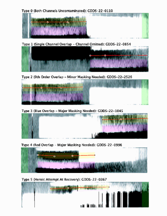
Figure 21: Examples illustrating the spectrum overlap classification system defined in Table 3. The transparent yellow and purple regions correspond to the negative and positive spectral extraction apertures.

As described in §2, our two-tier mask design strategy allowed some overlap to occur among spectra originating in adjacent slits. The extent of these overlaps can be gauged by an inspection of Figure 19. The wavelengths 5500–9200Å from the ‘blue tier’ spectra in second order can overlap with the first order ‘red tier’ spectra. Since 5500–9200Å is the main observational window, this second order light cannot be filtered out, nor is the second order sky cancelled in the Nod & Shuffle process, because the slits are in general not aligned between the two tiers. However the intensity of second order spectra in this wavelength range is only 5-10% of the intensity of the first order spectra, so in practice only the very strongest sky lines (such as [OI]5577Å, [OI]6300Å  and [OI]6363Å) were significant contaminants, and in many cases these individual lines can simply be masked out, as described above. Another source of contamination is zero-order light from red-tier spectra overlapping with the first-order spectra in the blue tier. Several examples of this contamination are clearly seen in Figure 19. Such cases are easy to identify and, as only a small portion of the spectrum is affected, this portion of the affected spectra has simply been eliminated in the final spectra presented in this paper. As noted earlier, we have attempted to classify the importance of spectrum overlaps using the system defined in Table 2. To help the reader visualize the meaning of this system, it is illustrated using example spectra in Figure 21.

C.5 Final ASCII-format Spectra

In addition to the main data tables presented in Tables 4 and 5 above, the GDDS Public Data Release contains the individual spectra for all galaxies in the survey. These spectra are stored as ASCII text files, each of which contains the eleven columns of information specified in Table 6. Linearly and optimally extracted calibrated spectra, their corresponding variance spectra, and an uncalibrated raw spectrum are stored in the same file. A linearly extracted night sky spectrum sampled through the same slit as part of the Nod & Shuffle operation is also included. All calibrated spectra have been fully processed through our pipeline; they are flux-calibrated, as well as corrected for atmospheric absorption and charge bleeding (via the ‘redfix’ correction described in §C.3). Separate columns in the output data file record the values of the atmospheric calibration, ‘redfix’, and flux calibration curves applied at each wavelength point in the spectrum (so the calibrations can be undone and new ones experimented with). A column in each file also records the fraction of masked pixels in the spatial direction at each wavelength. The final column in each file records raw counts in electrons normalized to the 1800s exposure time of a single sub-frame, as described above.

Table 6: Data Columns in Final Text-Format Spectrum Files

Name	Quantity	Unit
Lambda	Wavelength	Å
Flux	Linearly extracted object flux	erg ${\rm cm}^{-2}{\rm s}^{-1}{\rm\AA}^{-1}$
Sigma	Standard deviation of linearly extracted object flux	erg ${\rm cm}^{-2}{\rm s}^{-1}{\rm\AA}^{-1}$
SkyFlux	Linearly extracted sky flux	erg ${\rm cm}^{-2}{\rm s}^{-1}{\rm\AA}^{-1}$
OptFlux	Optimally extracted object flux	erg ${\rm cm}^{-2}{\rm s}^{-1}{\rm\AA}^{-1}$
OptSigma	Standard deviation of optimally extracted object flux	erg ${\rm cm}^{-2}{\rm s}^{-1}{\rm\AA}^{-1}$
RedFix	Additive correction for charge bleeding	counts
FluxCal	Flux calibration	mag
Atmos	Additive correction for atmospheric absorption	counts
Frac	Fraction of pixels masked in spectral dimension	$\cdots$
Electrons	Uncorrected counts	electrons

References

- Abraham et al. (2003) Abraham, R. G., et al. 2003. Gemini Newsletter, June 2003
- Bland-Hawthorn (1995) Bland-Hawthorn, J. 1995. In “Tridimensional Spectroscopic Methods in Astrophysics”, ed. Comté & Marcelin, M., ASP Conf., 71, 369.
- Chen et al. (2002) Chen, H–W., et al. 2002, 570, 54
- Cimatti et al. (2004) Cimatti, A. 2004. To appear in the Proceedings of the ESO/USM/MPE Workshop on “Multiwavelength Mapping of Galaxy Formation and Evolution”, eds. R. Bender and A. Renzini (astro-ph/0401101)
- Cimatti et al. (2003) Cimatti, A. et al. 2003, A&A, in press, (astro-ph/0310742)
- Cowie et al. (1994) Cowie, L. L., Gardner, J. P., Hu, E. M., Songaila, A., Hodapp, K.-W., & Wainscoat, R. J. 1994, ApJ, 434, 114
- Cuillandre et al. (1994) Cuillandre, J. C. et al. 1994. A&A, 281, 603
- Daddi et al. (2000) Daddi, E. et al. 2000. A&A, 361, 535
- Dunlop et al. (1996) Dunlop, J. et al. 1996. Nature, 381, 58
- Dunlop et al. (1999) Dunlop, J. S. 1999, in Rottgering H. J. A., Best P., Lehnert M. D., eds, The Most Distant Radio Galaxies. KNAW Colloq. Amsterdam. Kluwer, Dordrecht, p. 71
- Eisenstein et al. (2003) Eisenstein, D. J. et al. 2003, ApJ, 585, 694
- Ellis et al. (1996) Ellis, R. S., Colless, M., Broadhurst, T., Heyl, J., & Glazebrook, K. 1996, MNRAS, 280, 235
- Ellis (2001) Ellis, R. S. 2001. PASP, 113, 515
- Erb et al. (2003) Erb, D. K., Shapley, A. E., Steidel, C. C., Pettini, M., Adelberger, K. L., Hunt, M. P., Moorwood, A. F. M., & Cuby, J. 2003, ApJ, 591, 101
- Firth et al. (2001) Firth, A., et al. 2002, MNRAS, 332, 617
- Franx et al. (2003) Franx, M. et al. 2003, ApJ, 587, L79
- Glazebrook et al. (2004) Glazebrook, K. et al. (2004). Submitted to Nature. (astro-ph/0401037). [GDDS Paper III]
- Glazebrook et al. (2001) Glazebrook, K. & Bland-Hawthorn, J. 2001. PASP, 113, 197
- Hook et al. (2003) Hook, I. et al. 2003, Proc. SPIE, 4841, 1645
- Kauffmann et al. (1998) Kauffmann, G. & Charlot, S. 1998, MNRAS297, 23
- Lilly et al. (1995) Lilly, S. et al. 1995. ApJ, 455, 50
- Lilly et al. (1996) Lilly, S. et al. 1996. ApJ, 460, L1
- Lotz, Ferguson, & Bohlin (2000) Lotz, J. M., Ferguson, H. C., & Bohlin, R. C. 2000, ApJ, 532, 830
- Madau et al. (1996) Madau, P., Ferguson, H. C., Dickinson, M. E., Giavalisco, M., Steidel, C. C. & Fruchter, A. 1996, MNRAS, 283, 1388
- McCarthy et al. (2004) McCarthy, P. et al. 2004. In preparation. [GDDS Paper IV]
- McCarthy et al. (2001) McCarthy, P. et al. 2001, ApJ, 560, L131
- Murowinski et al. (2003) Murowinski, R. G. et al. 2003, Proc. SPIE, 4841, 1440
- Nagamine et al. (2003) Nagamine, K., Cen, R., Hernquist, L., Ostriker, J. P. & Springel, V. 2003. (astro-ph/0311294)
- Nolan, Dunlop, & Jimenez (2001) Nolan, L. A., Dunlop, J. S., & Jimenez, R. 2001, MNRAS, 323, 385
- Savaglio et al. (2004) Savaglio et al. 2004, ApJ, in press, (astro-ph/031043), [GDDS Paper II]
- Shapley et al. (2001) Shapley, A. E., Steidel, C. C., Adelberger, K. L., Dickinson, M., Giavalisco, M., & Pettini, M. 2001, ApJ, 562, 95
- Spinrad et al. (1997) Spinrad, H., Dey, A., Stern, D., Dunlop, J., Peacock, J., Jimenez, R., & Windhorst, R. 1997, ApJ, 484, 581
- Steidel et al. (1996) Steidel, C. C., Giavalisco, M., Pettini, M., Dickinson, M., & Adelberger, K. L. 1996, ApJ, 462, L17
- Steidel et al. (1999) Steidel et al. 1999. ApJ, 519, 1
- Steidel et al. (2003) Steidel, C. C., Adelberger, K. L., Shapley, A. E., Pettini, M., Dickinson, M., & Giavalisco, M. 2003, ApJ, 592, 728
- Tremonti et al. (2003) Tremonti, C. A., Leitherer, C., Heckamn, T. M., & Calzetti, D. 2003, ApJ, submitted.