Equilibria of a Self-Gravitating, Rotating Disk Around a Magnetized Compact Object

Abstract

We examine the effect of self-gravity in a rotating thick-disk equilibrium in the presence of a dipolar magnetic field. In the first part, we find a self-similar solution for non-self-gravitating disks. The solution that we have found shows that the pressure and density equilibrium profiles are strongly modified by a self-consistent toroidal magnetic field. We introduce 3 dimensionless variables $C_{B}$, $C_{c}$, $C_{t}$ that indicate the relative importance of toroidal component of magnetic field ($C_{B}$), centrifugal ($C_{c}$) and thermal ($C_{t}$) energy with respect to the gravitational potential energy of the central object. We study the effect of each of them on the structure of the disk. In the second part, we investigate the effect of self-gravity on the these disks; thus we introduce another dimensionless variable ($C_{g}$) that shows the importance of self-gravity. We find a self-similar solution for the equations of the system. Our solution shows that the structure of the disk is modified by the self-gravitation of the disk, the magnetic field of the central object, and the azimuthal velocity of the gas disk. We find that self-gravity and magnetism from the central object can change the thickness and the shape of the disk. We show that as the effect of self-gravity increases the disk becomes thinner. We also show that for different values of the star’s magnetic field and of the disk’s azimuthal velocity, the disk’s shape and its density and pressure profiles are strongly modified.

1 INTRODUCTION

The theory of accretion disks, motivated in a large degree by their occurrence in some binary systems, particularly cataclysmic variables, has been most fully developed for the thin Keplerian disks [Pringle 1981]. Based on their geometric shapes, accretion disks are generally divided into two distinct classes, thin disks and thick disks. The theory of thin accretion disks (Shakura & Sanyev 1973) is well understood whereas there is no universally accepted model for thick accretion disks. The current interest in this theory is due to the possibility that thick disks may be relevant to the understanding of central power sources in radio galaxies and quasars. Observational evidence suggests that in the center of many galaxies, matter is somehow ejected to large distances and gives off high energy radiation as it interacts with the external medium. There are other theoretical reasons for pursuing the study of thick disks. In the theory of thin disks, radial pressure gradients are neglected and vertical pressure balance is solved separately.It was shown that this approximation is valid as long as the disk is geometrically thin. This condition may be violated in the innermost region of accretion disks around stellar black holes and neutron stars. The study of thick disks provides a better theoretical understanding of thin disks as a limiting case and enables us to deal with intermediate situations [Frank et al. 1992]

When considering the formation process of astrophysical objects, such as galaxies and stars, the most crucial factor is self-gravity. In the standard thin accretion disk model, the effect of self-gravity is neglected, and only pressure supports the vertical structure. By contrast, the theory of self-gravitating accretion disks, is less developed. Early numerical work of self gravitating accretion disks began with N-body modelling (Cassen & Moosman 1991 ; Tomley, Cassen & Steinman-Cameron 1991). The time evolution of non-self-gravitating viscose disk has long been studied, and now we have a good theory describing its steady structure and its basic time-dependent behavior [Shakura & Sanyev 1973]; [Lyndenbell & Pringle 1974]. But with the added assumption of self-gravity in the disk, it is not easy to follow its dynamical evolution, mainly because the basic equations for the disks are highly nonlinear [e.g. Paczinsky 1978]; [Fukue & Sakamoto 1992]. To solve the nonlinear equations of self-gravitating disks, the technique of self-similar analysis is sometimes useful. Several classes of self-similar solutions were known previously, but all of them considered a disk in a fixed, external potential. Self-similar behavior provides an important class of solutions to the self-gravitating fluid equations. On the one hand, many physical problems often attained self-similar limits for a wide range of initial conditions. On the other hand, the self-similar properties allows us to investigate properties of solutions in arbitrary details, without any of the associated difficulties of numerical hydrodynamics.

Pen (1994) presented a general classification of self-similar self-gravitating fluids. Fukue & Sakamoto (1992) also analyzed the vertical structure of self-gravitating disks, but it is impossible to compare their models with realistic disks, because they computed the vertical structure using the thin-disk approximations for polytropes. Finally, using the numerically method proposed by Hachisu (1986) and Hachisu et al. (1987), Woodward et al. (1992) developed a code to investigate the interaction between a disk and its central object. However, they only considered polytropic disks. Hashimoto, Eriguchi & Muller (1995) presented a two-dimensional equilibrium model for self-gravitating Keplerian disks. They showed that the shape of the disk (or disk thickness) in flounced by the rotational law and the ratio of the disk mass to the mass of the central star. Bodo & Curir (1992)computed the equilibrium structure of a self-gravitating thick accretion disk by an iterative procedure which produced a final density distribution in equilibrium with the potential coming from it. They showed that the geometrical size and shape the disks influenced by self-gravity of the disk.

Accretion disks, containing magnetic fields, have been the subject of intense study in recent years. The role of the magnetic field in the equilibrium of accretion disks has been investigated by some authors [Blandford & zanjek 1997]; [Lubow, Papalizou & Pringle 1994] for the thin disk models , an ideal magneto hydrodynamics (MHD) equilibrium with azimuthal velocity and poloidal magnetic field has been analyzed [Lovelace et al. 1986]; [Mobarry & Lovelace 1986]. Using numerical methods, these authors found that the magnetic field may change the shape and angular momentum distribution in the disk. Thick disk configurations with a poloidal magnetic field has been studied by [Tripathy et al 1990], in the MHD framework [Banerjee, Bhatt, Das, Prasanna; 1995]. They investigated the equilibrium structure of thick disks and their stability in the presence of a dipolar magnetic field due to a non-rotating central object. Their solution shows that the pressure and the density equilibrium profiles are strongly modified by a toroidal magnetic field, resulting from the interaction between the permanent dipolar magnetic field and the inertia of the gas disk. In a magnetized disk, the inertia of the gas is expected to bend the magnetic field lines backwards, creating a toroidal component, which in turn may collimate a hydrodynamic outflow over long distances, forming jets. They assumed that the disk is non-accreting, stationary, axisymmetric, non-viscous, magnetized and that it is in equilibrium around a compact object, with only an azimuthal motion $V_{\phi}$.

We are interested in analyzing the role of self-gravity in thick disk equilibrium in the presence of the dipolar magnetic field of a central star. The outline of this paper is as follows: the general formalism of the problem is discussed in section 2, a self-similar solution of the equilibrium of non-self-gravitating accretion disks in the presence of a dipolar magnetic field is constructed in section 3, a self-similar solution of self-gravitating magnetized accretion disks is constructed in section 4 and a summary of the main ideas is given in section5.

2 GENERAL FORMALISM

As stated in the introduction, we are interested in analyzing the role of self-gravity in a thick disk equilibrium in the presence of the dipolar magnetic field of a central star. For simplicity, we ignore the influence of energy dissipation. We consider the disk as a non-accreting MHD flow around a magnetized , non rotating, central compact object. The disk is assumed to be stationary and axi-symmetric. We use a spherical polar, inertial, coordinate system, $(r,\theta,\phi)$, with origin fixed on the central object. The basic equations are two components of the euler equation in $(r,\theta)$ direction and poison’s equation:

$$\frac{\partial\Psi}{\partial r}=-\frac{1}{4\pi r}\frac{B_{\phi}}{\rho}\frac{\partial}{\partial r}(rB_{\phi})-\frac{GM}{r^{2}}-\frac{1}{\rho}\frac{\partial p}{\partial r}+\frac{V_{\phi}^{2}}{r},$$ (1)

$$\frac{\partial\Psi}{\partial\theta}=-\frac{1}{4\pi\sin\theta}\frac{B_{\phi}}{\rho}\frac{\partial}{\partial\theta}(B_{\phi}\sin\theta)-\frac{1}{\rho}\frac{\partial p}{\partial\theta}+V_{\phi}^{2}\cot\theta,$$ (2)

$$\frac{1}{r^{2}}\frac{\partial}{\partial r}(r^{2}\frac{\partial\Psi}{\partial r})+\frac{1}{r^{2}\sin\theta}\frac{\partial}{\partial\theta}(\sin\theta\frac{\partial\Psi}{\partial\theta})=4\pi G\rho,$$ (3)

where $\rho$, $p$, $V_{\phi}$, $B_{\phi}$ and $\Psi$ denote the gas density, pressure, toroidal velocity component, toroidal magnetic field, and gravitational potential respectively. Also G and M are the gravitational constant and the mass of central star. Solution of equations (1-3), in general, is a difficult task. Therefore, to simplify the problem, we impose two constraints. We adopt for $B_{\phi}$ and $V_{\phi}$ the same form as that given in ( Banerjee , Bhatt & Das; 1995). They assume that the magnetic field of the central star is dipolar:

$$B_{r}=2B_{0}(\frac{R}{r})^{3}\cos\theta,$$ (4)

$$B_{\theta}=B_{0}(\frac{R}{r})^{3}\sin\theta,$$ (5)

where $B_{0}$ is the magnetic field strength on the surface of the central star near the pole and $R$ is its radius. They showed that the dipolar field with the azimuthal motion of the gas disk, could make a toroidal component of the magnetic field, that is:

$$B_{\phi}=B_{1}(\frac{r}{R})^{(k-\frac{3}{2})}\sin^{-2k}\theta,$$ (6)

where $B_{1}$ is an arbitrary constant with the dimension of a magnetic field strength, and $k\leq\frac{3}{2}$ is a real constant. The general solution for $V_{\phi}$ is:

$$V_{\phi}=V_{0}(\frac{r}{R})^{(n+\frac{3}{2})}\sin^{-2n}\theta,$$ (7)

where $R$ denotes the radius of the star. $V_{0}$ is a constant with the dimension of a velocity and n is a real constant.

Now, we try to solve our equations with these constraints. At first we introduce $x$ according to :

$$x=\frac{r}{R_{d}},~{}~{}~{}~{}~{}~{}~{}~{}~{}~{}~{}\alpha=\frac{R_{d}}{R},$$ (8)

where $R$ and $R_{d}$ are the star and the disk radiuses respectively. Now we rewrite the Eqs.(6)-(7) as:

$$B_{\phi}=B_{1}\alpha^{k-\frac{3}{2}}~{}x^{k-\frac{3}{2}}~{}\sin^{-2k}\theta,$$ (9)

$$V_{\phi}=V_{0}\alpha^{n+\frac{3}{2}}~{}x^{n+\frac{3}{2}}~{}\sin^{-2n}\theta,$$ (10)

where $B_{1}$,$V_{0}$ are the strength of the toroidal component of the magnetic field and the rotational velocity on the surface of the star respectively. We can see clearly that the structure of the magnetic field of the central star can be modified by a rotational velocity of the gas disk.

2.1 MAGNETIC FIELD CONFIGURATION

In this subsection we want to study the magnetic field of central stars in the presence of a rotating gas disk. In a magnetized disk, magnetic field lines are deformed by the rotating gas. In this case, the gas is expected to be tied to the magnetic field lines and its inertia causes them to be bent backward and create a toroidal component.

To study the magnetic field configuration within the disk we will look at the magnetic field lines, which satisfy the following equation:

$$\frac{dr}{B_{r}}=\frac{rd\theta}{B_{\theta}}=\frac{r\sin\theta d\phi}{B_{\phi}},$$ (11)

In order to visualize the field line configurations, we now choose $k=-\frac{3}{2}$ in Eq.6. It is useful to express the results in a Cartesian frame through the usual relations ($X=r\sin\theta\cos\phi,Y=r\sin\theta\sin\phi,Z=r\cos\theta$). If we apply these transformations to the force equation we can obtain the corresponding parametric equations that generate the magnetic field configurations:

$$X=r_{in}\cos[\phi_{0}-\beta(\frac{r_{in}}{R})^{3}\cos\theta]\sin^{3}\theta,$$ (12)

$$Y=r_{in}\sin[\phi_{0}-\beta(\frac{r_{in}}{R})^{3}\cos\theta]\sin^{3}\theta,$$ (13)

$$Z=r_{in}\sin^{2}\theta\cos\theta,$$ (14)

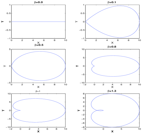
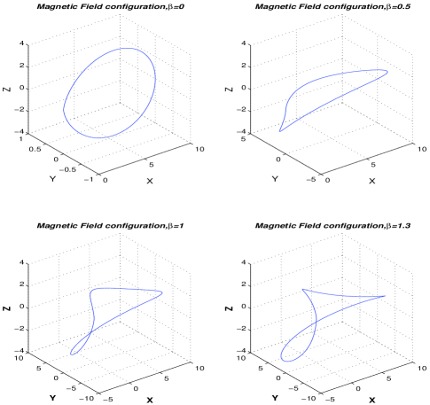
where $\Phi_{0}$ is a constant of integration (because we consider axi-symmetry solutions, we can set it to zero without any loss of generality), $\beta=\frac{B_{1}}{B_{0}}$ and $r_{in}$ is the disk inner radius. From the above equations we can see that the azimuthal component of the magnetic field can affect magnetic field line configurations in the disk. In Fig(1) we plot several 2-D field line configurations. We can see that when the toroidal component of the magnetic field is larger, the deformation of the magnetic field line is more obvious. In Fig.2 we plot several 3-D magnetic field configurations with the same parameters.

Figure 1: 2D Magnetic field configurations in a X-Y plane as a function of $\theta$, which runs from $\theta_{min}=0$ to $\theta_{max}=\pi$ ,at $r=r_{in}=10$ and R=7 for different value of $\beta=\frac{B_{1}}{B_{0}}$

Figure 2: 3D Magnetic field configurations as a function of $\theta$, which runs from $\theta_{min}=0$ to $\theta_{max}=\pi$ ,at $r=r_{in}=10$ and R=7 for different value of $\beta=\frac{B_{1}}{B_{0}}$

And now we come back to Eqs.(1-3) and introduce other dimensionless variables for the gravitational potential, the density and the pressure of the disk’s material:

$$S=\frac{\Psi}{\Psi_{0}},~{}~{}~{}~{}~{}~{}\Sigma=\frac{\rho}{\rho_{0}},~{}~{}~{}~{}~{}~{}\Lambda=\frac{p}{p_{0}},$$ (15)

where $\Psi_{0}$ , $\rho_{0}$ and $P_{0}$ are defined as:

$$\Psi_{0}=\frac{GM}{R_{d}}$$ (16)

$$\rho_{0}=\rho(r=R_{d},\theta=\frac{\pi}{2}),$$ (17)

$$p_{0}=p(r=R_{d},\theta=\frac{\pi}{2}),$$ (18)

By inserting these dimensionless parameters into Eqs.(1-2), and by performing some simplifications, we obtain:

$$\frac{\partial S}{\partial x}=-C_{B}\frac{x^{2k-4}}{\Sigma}(k-\frac{1}{2})\sin^{-4k}\theta+C_{c}x^{2n+2}\sin^{-4n}\theta$$

$$\\ -C_{t}\frac{1}{\Sigma}\frac{\partial\Lambda}{\partial x}-\frac{1}{x^{2}},$$ (19)

$$\frac{\partial S}{\partial\theta}=-C_{B}\frac{x^{2k-3}}{\Sigma}(-2k+1)\sin^{-4k+1}\theta\cos\theta$$

$$\\ +C_{c}x^{2n+3}\sin^{-4n}\theta\cot\theta-C_{t}\frac{1}{\Sigma}\frac{\partial\Lambda}{\partial\theta},$$ (20)

where $C_{B},C_{c},C_{t}$ are constants defined by:

$$C_{B}=\frac{\frac{B^{2}_{1}}{4\pi\rho_{0}}}{\frac{GM}{R_{d}}}\alpha^{2k-3},$$ (21)

$$C_{c}=\frac{V^{2}_{0}}{\frac{GM}{R_{d}}}\alpha^{2n+3},$$ (22)

$$C_{t}=\frac{\frac{P_{0}}{\rho_{0}}}{\frac{GM}{R_{d}}},$$ (23)

By introducing three dimensionless parameters indicating the relative importance of the energy of the toroidal component of the magnetic field ($C_{B}$), the centrifugal energy ($C_{c}$), the thermal energy ($C_{t}$) with respect to the gravitational potential energy of the central object, we can study them separately. If this simplification is used for Poisson’s equation, Eq.3, we find that:

$$\frac{1}{x^{2}}\frac{\partial}{\partial x}(x^{2}\frac{\partial S}{\partial x})+\frac{1}{x^{2}\sin\theta}\frac{\partial}{\partial\theta}(\sin\theta\frac{\partial S}{\partial\theta})=\frac{3M_{d}}{M}\Sigma,$$ (24)

where $M_{d}$ is the mass of the disk out to $R_{d}$:

$$M_{d}=\frac{4\pi}{3}R^{3}_{d}\rho_{0}$$ (25)

We may introduce another dimensionless variable $C_{g}$ that gives the importance of self-gravity. $C_{g}$ is the ratio of the disk mass to the central object mass:

$$C_{g}=\frac{3M_{d}}{M}$$ (26)

We would like to investigate self-similar solutions that describe the equilibrium structure of the thick disk. Thus we introduce self-similar solutions for the density and pressure of the gas disk:

$$\Sigma(r,\theta)=\frac{D(\theta)}{x^{\epsilon}}$$ (27)

$$\Lambda(r,\theta)=\frac{P(\theta)}{x^{\delta}}$$ (28)

Since we do not consider energy transport mechanisms, no specific form for the equation of state is assumed. As a result of our model we find that the density and pressure clearly show no polytropic, isothermal or other simple relation. We show that the indices in the non-self-gravitating and self-gravitating cases are completely different and that the mass distribution of the disk changes due to this fact. Solving Eqs.(19-20) and Eqs.(27-28) gives $\epsilon$ and $\delta$.

3 NON SELF-GRAVITATING SOLUTION

In this section we try to derive a self-similar solution of non-self-gravitating disks. In this regime we put $S$ equal to zero. If we put Eqs.(27-28) into Eqs.(19-20) we obtain:

$$-(k-\frac{1}{2})C_{B}x^{2k-4+\epsilon}\frac{\sin^{-4k}\theta}{D}+C_{c}x^{2n+2}\sin^{-4n}\theta$$

$$\\ +\delta C_{t}x^{\epsilon-\delta-1}\frac{P}{D}-\frac{1}{x^{2}}=0$$ (29)

$$(2k-1)C_{B}x^{2k-3+\epsilon}\frac{\sin^{-4k-1}\theta\cos\theta}{D}+C_{c}x^{2n+3}\sin^{-4n}\theta\cot\theta$$

$$\\ -C_{t}x^{\epsilon-\delta}\frac{1}{D}\frac{dP}{d\theta}=0$$ (30)

In order to obtain the indices of the self-similar solution, we require that in each equation the exponent of $x$ be the same for all the terms. Here we get:

$$2k-4+\epsilon=2n+2=\epsilon-\delta-1=-2$$ (31)

And we have:

$$\epsilon=2-2k$$ (32)

$$n=-2$$ (33)

$$\delta=-2k+3$$ (34)

These equations state that for getting a physical solution, $k$ must be less than unity. Then by putting the self-similar indices in the equations and by doing some simplifications, we obtain:

$$-(k-\frac{1}{2})C_{B}\frac{\sin^{-4k}\theta}{D}+C_{c}\sin^{8}\theta+(3-2k)C_{t}\frac{P}{D}-1=0$$ (35)

$$(2k-1)C_{B}\frac{\sin^{-4k-1}\theta\cos\theta}{D}+C_{c}\sin^{8}\theta\cot\theta-C_{t}\frac{1}{D}\frac{dP}{d\theta}=0$$ (36)

We have two equations with two unknowns. The first equation can be used to express $P$ as a function of $D$:

$$P(\theta)=\frac{1}{(3-2k)C_{t}}[(1-C_{c}\sin^{8}\theta)D(\theta)+(k-\frac{1}{2})C_{B}\sin^{-4k}\theta]$$ (37)

Figure 3: To the top left:Variation of density along the meridional as a function of $\theta$ from $\theta_{min}=0$ to $\theta_{max}=\pi$for different value of $C_{c}$ (rotational velocity), Top right: for deferent value of $k$, bottom left: Iso-density contour for different value of $C_{c}$, Bottom right: variation of pressure with different value of $C_{c}$

With our definitions of $\rho_{0}$ and $P_{0}$, we have $D(\theta=\frac{\pi}{2})=1$ and $P(\theta=\frac{\pi}{2})=1$. If we introduce this boundary condition in Eq.37, $C_{t}$ can be calculated:

$$C_{t}=\frac{1}{(3-2k)}[1-C_{c}+(k-\frac{1}{2})C_{B}],$$ (38)

Now if we introduce Eq.37 into 36, we find:

$$\frac{dD}{d\theta}=g(\theta)D+f(\theta),$$ (39)

where:

$$g(\theta)=(11-2k)\frac{C_{c}\sin^{7}\theta\cos\theta}{1-C_{c}\sin^{8}\theta},$$ (40)

$$f(\theta)=3(2k-1)C_{B}\frac{\sin^{-4k-1}\theta\cos\theta}{1-C_{c}\sin^{8}\theta},$$ (41)

For this equation we do the following change of variable:

$$D(\theta)=[1-C_{c}\sin^{8}\theta]^{-\frac{11-2k}{8}}D_{1}(\theta),$$ (42)

$$\frac{dD_{1}(\theta)}{d\theta}=[1-C_{c}\sin^{8}\theta]^{\frac{11-2k}{8}}f(\theta),$$ (43)

or:

$$\frac{dD_{1}(\theta)}{d\theta}=3C_{B}(2k-1)[1-C_{c}\sin^{8}\theta]^{\frac{3-2k}{8}}\sin^{-4k-1}\theta\cos\theta,$$ (44)

The solution of this equation can be write as:

$$D_{1}(\theta)=3C_{B}(2k-1)I(\theta)+D_{01},$$ (45)

where:

$$I(\theta)=\int^{\theta}_{0}[1-C_{c}\sin^{8}\theta^{{}^{\prime}}]^{\frac{3-2k}{8}}\sin^{-4k-1}\theta^{{}^{\prime}}\cos\theta^{{}^{\prime}}d\theta^{{}^{\prime}};$$ (46)

Now we come back to our boundary conditions for the density. The maximum density is at $\theta=\frac{\pi}{2}$ where $D(\frac{\pi}{2})=1$. Now we can find the value of $D_{01}$ as:

$$D_{1}(\frac{\pi}{2})=[1-C_{c}\sin^{8}\theta]^{\frac{11-2k}{8}}|_{\theta=\frac{\pi}{2}}D(\frac{\pi}{2})=[1-C_{c}]^{\frac{11-2k}{8}};$$ (47)

Thus:

$$D_{01}=[1-C_{c}]^{\frac{11-2k}{8}}-3C_{B}(2k-1)I(\theta=\frac{\pi}{2});$$ (48)

Hence we can find the density distribution:

$$D(\theta)=[(1-C_{c})^{\frac{11-2k}{8}}-3C_{B}(2k-1)(I(\frac{\pi}{2})-I(\theta))]$$

$$\\ \times[1-C_{c}\sin^{8}\theta]^{-\frac{11-2k}{8}};$$ (49)

The important result from this equation is that the value of the density is not zero in the rotation axis. This value depends on our dimensionless parameters, $C_{B}$ and $C_{c}$, where $C_{B}$ represents the effect of the toroidal component of the magnetic field and $C_{c}$ the effect of the rotation velocity.

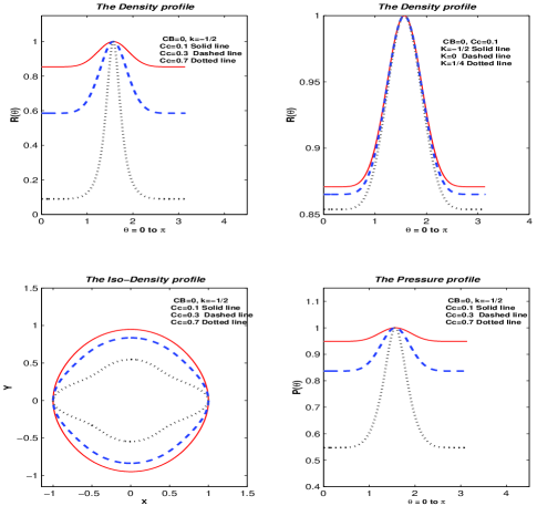
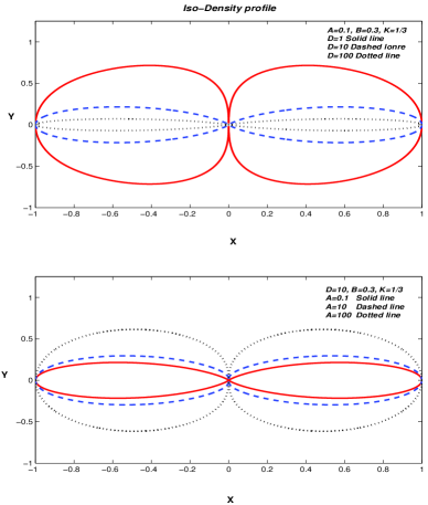
Fig(3) shows typical examples of the self-similar solution in equations (37) and (49). In Fig(3), the density profiles, the iso-density contours and the variations of pressure along the meridional axes are represented. The density profiles for different values of $C_{c}$ (rotational velocity) and $k$ are displayed. As can be seen, the parameter $C_{c}$ determines the overall shape of the matter distribution. By increasing the effect of the rotational velocity ($C_{c}$), the shape of the disk changes to a thinner one, which is due to centrifugal force. In Fig(3), we also present the iso-density contours for the same value of $C_{c}$. As can be seen, the shape of the disk is strongly modified for different values of $C_{c}$. We can see that in this case, the density does not vanish at $\theta=0,\pi$ (in the rotational axes). Our solution agrees with [Banerjee, Bhatt, Das, Prasanna; 1995] solutions for such systems.

We should mention that the solution we have found is a mathematical one. As a result, the solution has a physical meaning only for parts of the parameter space. In this self-similar solution we have a singularity in $\theta=0,\pi$ that arises from $\sin\theta$ in the integral of equation (46); Thus we cannot study the effect of the magnetic field in the equilibrium structure of the gas disk. That is the nature of the solution. After we have found the analytical solution for non-self-gravitating disks, we will try to investigate the effect of self-gravity in such disks.

4 SELF-GRAVITATING SOLUTION

In order to gain a better understanding of the physical situation of the disk, we include self-gravity in the above equations. The self-similar technique is utilized once again. If we introduce Eq.(27-28) in to Eq. (19-20) we obtain:

$$\frac{\partial S}{\partial x}=-C_{B}(k-\frac{1}{2})x^{2k-4+\epsilon}\frac{\sin^{-4k}\theta}{D(\theta)}+C_{c}x^{2n+2}\sin^{-4n}\theta$$

$$\\ +\delta C_{t}x^{\epsilon-\delta-1}\frac{P(\theta)}{D(\theta)}-\frac{1}{x^{2}};$$ (50)

$$\frac{\partial S}{\partial\theta}=-C_{B}(-2k+1)x^{2k-3+\epsilon}\frac{\sin^{-4k-1}\theta\cos\theta}{D(\theta)}$$

$$\\ +C_{c}x^{2n+3}\sin^{-4n}\theta\cot\theta-C_{t}x^{\epsilon-\delta}\frac{1}{D(\theta)}\frac{dP(\theta)}{d\theta};$$ (51)

For finding the self-similar solution we must set equal the terms that have the same power. We obtain:

$$\epsilon=\frac{5-2k}{2}$$ (52)

$$n=\frac{2k-7}{4}$$ (53)

$$\delta=3-2k$$ (54)

Now we can identify the radial dependence of the density and pressure of the gas disk ($\epsilon$ and $\delta$ ) as functions of $k$. We can insert Eqs.(50-51) into Eq.(24) with use Eq.(27) we can find:

$$\frac{\partial S}{\partial x}=H(\theta)x^{\frac{2k-3}{2}}-\frac{1}{x^{2}},$$ (55)

$$\frac{\partial S}{\partial\theta}=W(\theta)x^{\frac{2k-1}{2}},$$ (56)

where we used a $k$ as a free parameter and:

$$H(\theta)=[-(k-\frac{1}{2})C_{B}\frac{\sin^{-4k}\theta}{D(\theta)}+C_{c}\sin^{-2k+7}\theta$$

$$~{}~{}~{}~{}~{}~{}~{}~{}~{}~{}~{}~{}~{}~{}~{}~{}~{}~{}~{}~{}~{}~{}~{}~{}~{}~{}~{}~{}~{}~{}~{}~{}~{}~{}+(3-2k)C_{t}\frac{P(\theta)}{D(\theta)}],$$ (57)

$$W(\theta)=[C_{B}(-2k+1)\frac{\sin^{-4k-1}\theta\cos\theta}{D(\theta)}+C_{c}\sin^{-2k+7}\theta\cot\theta$$

$$~{}~{}~{}~{}~{}~{}~{}~{}~{}~{}~{}~{}~{}~{}~{}~{}~{}~{}~{}~{}~{}~{}~{}~{}~{}~{}~{}~{}~{}~{}~{}~{}~{}~{}~{}~{}~{}~{}-C_{t}\frac{1}{D(\theta)}\frac{dP}{d\theta}],$$ (58)

Now if we introduce Eqs.(55-56) into Eq. (24) and do some simplifications, we obtain an ordinary differential equation with two unknown functions ($D(\theta)$ and $P(\theta)$):

$$(\frac{2k+1}{2})H(\theta)+\frac{1}{\sin\theta}\frac{d}{d\theta}[\sin\theta W(\theta)]=\frac{3M_{d}}{M}D(\theta)$$ (59)

In order to solve this equation, we need another relation between $D(\theta)$ and $P(\theta)$. By looking at the definitions of $H~{}\&~{}W$, we can find:

$$\frac{2}{2k-1}\frac{dH}{d\theta}=W(\theta),$$ (60)

Figure 4: Variation of the density of the disk for several values of the parameters: the top one: is for different values of $C_{B}$ that represents the importance of the magnetic field; the middle one: for different values of $C_{g}$ that represents the importance of self-gravity; the bottom one: is for different values of $C_{c}$ that represents the importance of the rotational velocity

Figure 5: Iso-density contours of the self-gravitating disks: the top one: for different values of $C_{g}$ that represents the importance of self-gravitation; the bottom: for different values of $C_{B}$ that represents the importance of the magnetic energy.

Now by solving Eqs. (59-60) we can find the angular dependence of the density and pressure of the gas disk ($D,P$). We linearize these equations, introduce another dimensionless constant defined as the ratio of the disk mass to the mass of the central object ($C_{g}$), and we use $Q=\frac{1}{D}$ instead of $D$ in order to simplify the equations. Thus with some calculations, we get:

$$\frac{dy_{1}}{d\theta}=S(\theta,y_{1},y_{2},y_{3});$$ (61)

$$\frac{dy_{2}}{d\theta}=y_{3};$$ (62)

$$\frac{dy_{3}}{d\theta}=T(\theta,y_{1},y_{2},y_{3});$$ (63)

where $y_{1}=Q=\frac{1}{D}$, $y_{2}=P$, $y_{3}=\frac{dP}{d\theta}$, and $S$ and $T$ are complex functions of $\theta$ , $y_{1}$, $y_{2}$, $y_{3}$. We solve these linear equations, with two point boundary conditions with the shooting method. Solving these equations gives the meridional component of the density and pressure. We used Naryan & Yi (1995) boundary conditions:

$$\frac{d\rho}{d\theta}\mid_{\theta=0}=\frac{d\rho}{d\theta}\mid_{\theta=\frac{\pi}{2}}=0$$ (64)

$$\frac{dp}{d\theta}\mid_{\theta=0}=\frac{dp}{d\theta}\mid_{\theta=\frac{\pi}{2}}=0$$ (65)

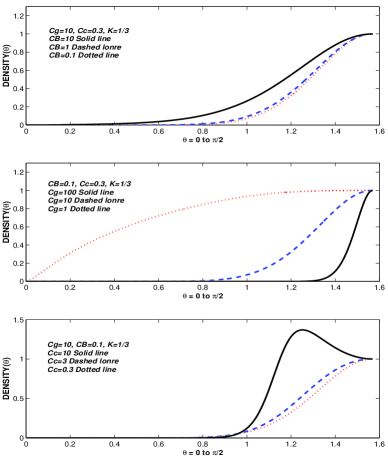
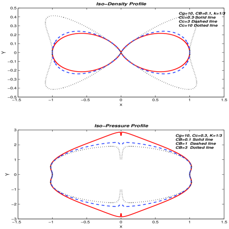
By changing the value of the dimensionless parameters $C_{B}$, $C_{c}$, $C_{t}$ and $C_{g}$, we can study the influence of the toroidal magnetic field, toroidal velocity, thermal energy and self-gravity of the gas disk on its own equilibrium structure. In Fig( 4-6) we plot some of our results. By comparing the results in Fig(4-5) which are calculated for different values of $C_{g}$, we can see how the disk is more sensitive to the influence of self-gravity. Fig(4) shows the variations of the density for different values of $C_{g}$ , $C_{B}$, $C_{c}$ in meridional direction. Concerning the geometrical shape of the disk we can see the tendency of the disk to become thinner when self-gravity plays an important role ($C_{g}$ is large). And then we can see that a strong magnetic field coming from the central star can produce a large toroidal component, which can change the thickness of the disk near the pole. Fig(4) shows the iso-density contours of the disk for different values of $C_{g}$ and $C_{B}$. In Fig(6) we present the iso-density profile of the disk for different values of $C_{c}$ and the iso-pressure profile of the disk for different values of $C_{B}$. We can see in the iso-pressure profile that near the pole there is a singularity; maybe this big pressure gradient could produce a jet from the pole! In order to test this effect we should investigate the time evolution of such systems. This could be the subject of future works.

Concerning the ratio of the mass of the disk to the mass of the central star, Eriguchi & Muller (1993) extended their code to include a central object for a thick disk and calculated the equilibrium structure of the disk which rotates according to the $j$-const law, where $j$ is the specific angular momentum. Comparing this with the toroidal star of Hashimito et al. (1993), where the central object is not included, the relative thickness of the disk is smaller, which is caused by effects due to gravity of the central star (see figures in Eriguchi & Muller 1993). As for the rotation law, Hashimito et al. (1993) and Eriguchi & Muller (1993) obtained rather thick disks, while Hashimito et al. (1995) found a flat disk shape where the gravitational force of the central object becomes relatively week compared with the self-gravity of the disk. Our results agree with the latter one. We can see in Fig(4-6) that the shape of the disk (or disk thickness) is influenced by the rotational law and the ratio of the disk mass to the mass of the central star.

Figure 6: Iso-density contours of the self-gravitating accretion disks: the top one: for different values of $C_{c}$, which represents the importance of rotational velocity; the bottom one: iso-pressure contours of the disk for different values of $C_{B}$, which represents the importance of the magnetic field.

5 DISCUSSION AND CONCLUSIONS

In this paper, we find a global equilibrium of a self-gravitating disk around a magnetized compact object. We ignore the effects of energy dissipation and radial flow. We have investigated a stationary model for a self-gravitating disk influenced by a strong magnetic field coming from the central object. We ignore the effects of the local magnetic field of the disk. We consider that the radial flow is negligible with respect to the azimuthal motion of the gas in the disk. We find two types of self-similar solutions for such disks. The first one is the non-self-gravitating self-similar solution that shows that the shape of the disk changes when the physical parameters are modified. The second one is the self-gravitating self-similar solution. In this class of solutions we can study the effect of self-gravity on the shape and thickness of the disk.

In the non-self-gravitating solution we find an analytical solution for some parts of the parameter space. This solution is found with a self-similarity method, and it gives a picture of the equilibrium structure of the gas material around a magnetized compact object. The solution shows that the rotational velocity of the gas disk can change the equilibrium picture. The important result that can be inferred from this solution is the non-vanishing value of the density on the rotation axis. This value depends on the dimensionless parameters, $C_{B}$ and $C_{c}$, where $C_{B}$ represents the effect of the magnetic field and $C_{c}$ the effect of the rotational velocity.

In the self-gravitating solution, we find the vertical (meridional) dependence of the gas density in the disk Fig(4). The external dipole field can change the thickness of the disk near the pole, and the existence of a sharp density gradient in the $\theta$-direction indicates a rapid decrease of the matter density away from the equatorial plane. But when self-gravity plays an important role in the disk equilibrium (by increasing $C_{g}$) we can see that the thickness of the disk decreases.

In Fig(5-6) we show some iso-density and iso-pressure contours of the equilibrium configuration of the disk for different values of $C_{B}$, $C_{c}$, $C_{g}$, $k$. In the iso-pressure profile we can see a large pressure gradient near the poles, which may lead to outflows in those regions! This idea would require further study, such as a dynamical investigation.

We see that the presence of self-gravity in a thick disk, can change the geometrical shape of the disk and plays an important role in equilibrium structure of the disk. We also see that the strength of the magnetic field can change the structure of the disk near the poles. Finally, we must admit that our model does not deserve the name ”accretion” disk, since we did not include the accretion (mass) flow.

This study, one of the first of its kind, is a search for an equilibrium structure of a thick disk in the presence of an external stellar dipole along with a self-consistently generated toroidal magnetic field $B_{\phi}$. The meridional structure of the disk is mainly due to the balance of plasma pressure gradient, magnetic force due to $B_{\phi}$, and centrifugal force. The existence of an equilibrium structure, in fact, encourages one to look for generalizations of the analysis to the case when the radial velocity $V_{r}\neq 0$, representing accretions. On the other hand, yet another important aspect to be considered is the generalization of the newtonian analysis to general relativistic formalism wherein space-time curvature produced by the strong gravitational field of the central object would modify the magnetic fields and introduce new features.

Our disk model might also apply to systems where the central object is a black hole, a neutron star or an active galactic nucleus. However, in this paper we modelled the disk under the assumption of a Newtonian potential. For a system where the central object is a black hole, the pseudo-Newtonian potential will play an essential role near the central object. The modification arising from a pseudo-Newtonian potential to the disk will be investigated in a future paper. Consequently, we cannot calculate the accretion luminosity. Thus, to compare our results with other models or observations, it will be necessary to include mass flow in our model.

We are grateful to the referee for a very careful reading of the manuscript and for suggestions which help us improve the presentation of our results. We are grateful Mohsen Shadmehri for continuous encouragement and useful discussions. We thank Kattia Ferriere, Daniel Reese and saeed farivar for their useful comments.

References

- [Abramovicz et al. 1987] Abramovicz, 1987, Comm.Astrophys., 12, 67
- [Adams, Lada, Shu1987] Adams, Lada, shu, 1987, Apj, 321, 788
- [Balbus & Haweley 1991] Balbus, & Haweley, 1991, Rev. Mod. Phys.
- [Banerjee, Bhatt, Das, Prasanna; 1995] Banerjee, Bhatt, Das, Prasanna 1995, Apj, 449, 789
- [Blandford & Payne 1982] Blandford & Payne. 1982, M.N.R.A.S, 199, 883
- [Blandford & zanjek 1997] Blandford, zanjek 2001, M.N.R.A.S, 179, 433
- [Bodenheimer et al. 1978] Bodenheimer, 1978, Apj, 224, 488
- [Bardou, Hyverts, Duschl 1998] Bardou, Hyverts, Duschl. 1998, A&A, 337, 996
- [Bertin & Lodato 1999] Bertin, Lodato, 1999, A&A, 350,694B
- [Bodo & Curir 1992] Bodo, Curir, 1992, A&A, 253,318
- [Cassen & Moosman 1991] Cassen, Moosman, 1991, Ikarus, 48, 353
- [Duschl & strittmatter & Bierman 2000] Duschl, strittmatter, Bierman, 2000, A&A, 253,318
- [] Eriguchi, Y, Muller 1993 ,ApJ, 416, 666
- [Frank et al. 1992] Frank, Accretion power in astrophysics, 1992, cambridge university press
- [Fukue & Sakamoto 1992] Fukue,J., Sakamoto, C. 1992, PASJ, 44, 553
- [] Hachisu, I, 1986,ApJS, 61 479
- [] Hachisu, I, 1986,ApJS, 62 461
- [] Hachisu, I., Eriguchi, Y., Muller, E., 1995, A&A, 297, 135
- [] Hashimoto, M., Tohline, J,E., Eriguchi, Y., 1987, ApJ, 323, 592
- [] Hashimoto, M., Eriguchi, Y., Arai, K., Muller, E., 1993, A&A, 268,131
- [] Hashimoto, M., Eriguchi, Y., Muller, E., 1995, A&A, 297,135
- [Lubow, Papalizou & Pringle 1994] Lubow, Papalizou, Pringle, 1994, M.N.R.A.S, 152, 461
- [Lyndenbell & Pringle 1974] Lyndenbell, Pringle, 1974, M.N.R.A.S, 168, 603
- [Lovelace et al. 1986] Lovelace, 1986, ApjS, 62, 1
- [Mobarry & Lovelace 1986] Mobarry, Lovelace, 1986, Apj, 309, 455
- [] Narayan , R., Yi, I., 1995, Apj, 444, 231
- [papalizu & pringle 1984] Papalizu, Pringle, 1984, M.N.R.A.S, 208, 721
- [e.g. Paczinsky 1978] Pringle, 1981, Ann. Rev. Astron. Astr., 19, 137
- [] Pen, U., 1994, ApJ, 429, 759
- [Pringle 1981] Paczynsky, B. 1978, Acta Astron., 28, 91
- [Shakura & Sanyev 1973] Shakura, Sanyev, 1973, A&A, 24, 337
- [Tripathy et al 1990] Tripathy, S. C., 1990, M.N.R.A.S, 246, 384