A three-dimensional model for the radio emission of magnetic chemically peculiar stars

In this paper we present a three-dimensional numerical model for the radio emission of Magnetic Chemically Peculiar stars, on the hypothesis that energetic electrons emit by the gyrosynchrotron mechanism. For this class of radio stars, characterized by a mainly dipolar magnetic field whose axis is tilted with respect to the rotational axis, the geometry of the magnetosphere and its deformation due to the stellar rotation are determined. The radio emitting region is determined by the physical conditions of the magnetosphere and of the stellar wind. Free-free absorption by the thermal plasma trapped in the inner magnetosphere is also considered. Several free parameters are involved in the model, such as the size of the emitting region, the energy spectrum and the number density of the emitting electrons, and the characteristics of the plasma in the inner magnetosphere. By solving the equation of radiative transfer, along a path parallel to the line of sight, the radio brightness distribution and the total flux density as a function of stellar rotation are computed. As the model is applied to simulate the observed 5 GHz lightcurves of HD 37479 and HD 37017, several possible magnetosphere configurations are found. After simulations at other frequencies, in spite of the large number of parameters involved in the modeling, two solutions in the case of HD 37479 and only one solution in the case of HD 37017 match the observed spectral indices. The results of our simulations agree with the magnetically confined wind-shock model in a rotating magnetosphere. The X-ray emission from the inner magnetosphere is also computed, and found to be consistent with the observations.

Figure 1: Cross-section of the magnetosphere of magnetic chemically peculiar stars: the stellar dipolar field (short dashed curves) is modified by the stellar wind; inside the Alfvén surface (long dashed curve), the magnetic pressure exceeds the kinetic pressure of the wind, and the field lines maintain a dipolar geometry. The largest closed field line defines the “inner” magnetosphere, which confines the stellar wind (“dead zone”). Here the two stellar wind streams from opposite hemispheres of the stellar surface collide, leading to a shock that produces an enhancement of the temperature of the gas and eventually to X-ray emission. This gas cools and accumulates in the magnetic equatorial plane, forming a torus-like cloud (the two filled circles close to the star). The open magnetic field lines just outside the inner magnetosphere produce current sheets (shaded areas), where the electrons are accelerated up to relativistic energies. They eventually can propagate back toward the stellar surface following the field lines of the “middle” magnetosphere and emit radio radiation by the gyrosynchrotron emission process (wave arrows). The hot matter in the inner magnetosphere can absorb the radio radiation. The field lines close to the magnetic poles of the star are open (“outer” magnetosphere), and tend to a radial topology outside the Alfvén surface. Only the wind from the polar caps can escape from the magnetosphere.

1 Introduction

Magnetic Chemically Peculiar (MCP) stars are commonly characterized by strong ($B\sim 10^{3}$ – $10^{4}$ Gauss) and periodically-variable surface magnetic fields. The observed magnetic variability is related to the global magnetic field topology of these stars which is mainly dipolar, with the magnetic axis tilted with respect to the rotational axis. The observed variability is a simple consequence of stellar rotation (Babcock Babcock49 (1949)).

These stars show evidence of anisotropic winds, as indicated by spectral observations of UV lines (Shore et al. shore_et_al (1987), Shore & Brown sho_e_bro (1990)). Theoretical studies have demonstrated that a stellar wind in the presence of a dipolar magnetic field can freely flow only from the polar regions, where the magnetic field lines are open (Shore shore (1987)). Therefore in MCP stars the wind forms two polar jets, whereas at the latitudes near the magnetic equator the wind is inhibited and the matter is trapped, forming the so called “dead zone”. The presence of jets and circumstellar matter can explain the emission features observed in the UV spectra and $H_{\alpha}$ wings (Walborn walborn (1974)). In some cases the mass loss rate ($\dot{M}=10^{-9}$ – $10^{-10}\leavevmode\nobreak\ M_{\sun}\mathrm{yr}^{-1}$) and the outflow terminal speed ($v_{\infty}\simeq 600$ km s^-1) was derived (Shore et al. shore_et_al (1987), Groote & Hunger gro_e_hun (1997)).

About 25% of MCP stars also show evidence of non-thermal radio continuum emission (Drake et al. drake_et_al (1987), Linsky et al. linsky_et_al (1992), Leone et al. leone_et_al (1994)). It has been suggested that the physical processes responsible for the observed radio emission are strictly related to the interaction between wind and magnetic field (Linsky et al. linsky_et_al (1992), Babel & Montmerle 1997a , hereafter BM97). The flat spectral index and the observed degree of circular polarization have been interpreted in terms of gyrosynchrotron emission from continuously injected mildly relativistic electrons trapped in the stellar magnetosphere.

The radio emission of MCP stars is variable with the same period as the magnetic field variability, as shown by Leone (leone (1991)) and Leone & Umana (leo_e_uma (1993)) for HD 37479 and HD 37017, and by Lim et al. (lim (1996)) for HR 5624. In particular, for HD 37479 and HD 37017, the minimum of the radio emission coincides approximately with the zero of the longitudinal magnetic field, whereas the maxima coincide with the extremes of the magnetic field curves (Leone & Umana leo_e_uma (1993)). The observed modulation suggests that the radio emission arises from a stable corotating magnetosphere. The temporal variability of the radio flux is probably related to the change of the orientation of the emitting region in the space, due to the misalignment of magnetic and rotational axes.

In this paper we present a three-dimensional gyrosynchrotron model developed with the aim of investigating the nature of the rotational modulation of the radio emission. This kind of study can be used to test the physical scenario proposed to explain the origin of radio emission from MCP stars.

2 The model

To explain the radio continuum and the X-ray emission from young magnetic B stars and MCP stars, André et al. (andre_et_al (1988)) proposed a model characterized by the interaction between the dipolar magnetic field and the stellar wind. Close to the star, where the magnetic pressure dominates over the kinetic pressure of the wind, the magnetic topology is mainly dipolar. As the magnetic field strength decreases, the kinetic pressure equals the magnetic one, defining the Alfvén surface, and the wind opens the magnetic field lines, generating a “current sheet” in the magnetic equatorial plane (Havnes & Goertz hav_e_goe (1984)). Here the electrons of the wind can be accelerated up to relativistic energies (Usov & Melrose uso_mel (1992)); eventually those electrons return to the star, along the field lines, thus defining the gyrosynchrotron emitting region. In the magnetosphere we identify three main zones:

• the “inner” magnetosphere or “dead zone”, completely inside the Alfvén surface, defined by the largest closed magnetic line; here the wind is confined;

• the “middle” magnetosphere, where the radio emission occurs, holding all the open magnetic field lines that generate the current sheets;

• the “outer” magnetosphere, where the wind flows freely from the magnetic polar caps, with a magnetic topology almost radial out of the Alfvén surface.

Linsky et al. (linsky_et_al (1992)) located as possible radio emitting regions two tori, one in the northern, the other in the southern magnetic hemisphere, inside the “middle” magnetosphere, the higher frequency being generated closer to the star, where the magnetic field is stronger.

The recent discovery of coherent emission at 20 cm from HD 124224 by Trigilio et al. (trigilio (2000)), explained in terms of Electron Cyclotron Maser Emission (ECME), seems to confirm the hypothesis of relativistic electrons accelerated in the current sheets and returning toward the star, where they are reflected back. In fact the ECME can occur after the magnetic mirroring when, in particular conditions, a loss cone anisotropy can develop (Melrose & Dulk meldulk (1982)).

The basic scenario of the magnetosphere of a MCP star is sketched in Fig. 1. If this scenario is correct, it should also reproduce the rotational modulation of the observed radio emission. We outline the basic steps of the model in Appendix A.1, while the stellar reference frame and its rotation are presented in Appendix A.2 and A.3. The numerical computation of the radio emission toward the Earth is presented in Appendix B.1. In the following, we analyze the numerical sampling of the emitting region, and the physical conditions of the magnetosphere.

2.1 Sampling

The space surrounding the star is sampled in a 3-D cubic grid (see Appendix A.2) and all the physical quantities relevant for the numerical computation of the radio emission (such as magnetic field, electron density,…) are evaluated in each grid point.

Since the frequency of the gyrosynchrotron radiation is proportional to the gyration frequency of the electrons, which in turn is proportional to the magnetic field intensity, different frequencies are mainly emitted in different regions of the magnetosphere at different distances from the stellar surface, because of the strong gradient of $B$ in a dipole. Therefore the modelled region is a cube whose overall size is a function of the frequency. This cube is then sampled into smaller cubes, whose size is chosen so that any physical parameter inside them can be assumed constant.

The reliability of the model is obviously greater if the size of the cube element is smaller but, on the other hand, the computational time increases strongly. The compromise between sampling and computational time is chosen on the basis of the convergence of the model (the flux for instance) as a function of the sampling toward an asymptotic value. In particular, to model the 5 GHz radiation from the MCP stars, the overall linear size of the grid is $25-30$ stellar radii, divided into about $80-100$ cube elements.

2.2 Location of the Alfvén surface

Figure 2: Thermal electron number density (top panel), magnetic field strength (medium panel) and equatorial radius of the Alfvén surface (low panel) versus magnetic longitude $\zeta$. They are derived with $R_{\ast}=4\leavevmode\nobreak\ R_{\sun}$, $P_{\mathrm{rot}}=1$ day, $B_{\mathrm{p}}=10^{4}$ Gauss, $\beta=60\degr$, $\dot{M}=10^{-9}\leavevmode\nobreak\ M_{\sun}\mathrm{yr}^{-1}$ and $v_{\infty}=600$ km s^-1, see Sect. 2.2 for details.

The equatorial radius of the Alfvén surface ($r_{\mathrm{A}}$) may be estimated by equating the kinetic energy density $\varepsilon_{\mathrm{w}}$ and the magnetic energy density $\frac{B^{2}}{8\pi}$ (Usov & Melrose uso_mel (1992)):

$$\varepsilon_{\mathrm{w}}=\frac{B^{2}}{8\pi}$$ (1)

The term $\varepsilon_{\mathrm{w}}$ includes both radial and rotational components of the kinetic energy of the wind:

$$\varepsilon_{\mathrm{w}}=\frac{1}{2}\rho v^{2}+\frac{1}{2}\rho\omega^{2}d^{2}$$ (2)

where $\rho$ and $v$ are the density and the speed of the wind respectively, $\omega$ is the angular velocity of the star and $d$ the distance of the generic point of the magnetic equator from the rotational axis, given by:

$$d=r\sqrt{1-\sin^{2}\beta\cos^{2}\zeta}$$

where $\beta$ is the obliquity of the magnetic field, $\zeta$ is the magnetic longitude (defined to be zero in the line located by rotational and magnetic equator planes) and $r$ the radial distance from the centre of the star. The gas density $\rho$ in the “outer” region can be estimated by the continuity equation:

$$\rho=\frac{\dot{M}}{4\pi r^{2}v(r)}$$ (3)

where $\dot{M}$ is the mass loss rate. The wind speed $v$ is a function of the distance from the star. For the sake of simplicity, we use the wind speed function derived by Castor & Simon (cas_e_sim (1983)):

$$v(r)=v_{\infty}\left(1-\frac{R_{\ast}}{r}\right)$$ (4)

This equation is similar to the velocity law $v(r)=v_{\infty}\left(1-R_{\ast}/r\right)^{0.8}$ theoretically predicted by Friend & Abbott (fri_e_abb (1986)) for a radiatively driven stellar wind. However, we emphasize that the above dependence of the stellar wind on the distance applies only for the “outer” and “middle” magnetosphere, while we expect a different velocity and density distribution in the “dead zone” (see Sect. 2.4), as the close magnetic flux tubes strongly influence the dynamics of the trapped wind (BM97).

To estimate the magnetic energy density in the equatorial plane of the “inner” magnetosphere, we use the expression of the strength for a dipolar field:

$$B=\frac{1}{2}B_{\mathrm{p}}\left(\frac{R_{\ast}}{r}\right)^{3}$$ (5)

where $B_{\mathrm{p}}$ is the strength of the magnetic field at the pole of the star.

Substituting Eqs.(2) and (5) in Eq.(1) we derive the equatorial Alfvén radius $r_{\mathrm{A}}$ as a function of the magnetic longitude $\zeta$ searching the real roots. The equatorial Alfvén radius ($r_{\mathrm{A}}$), the corresponding magnetic field strength ($B_{\mathrm{A}}$) and the thermal electron number density ($n_{\mathrm{e,A}}$) are plotted in Fig. 2 as a function of $\zeta$. They are derived for $R_{\ast}=4\leavevmode\nobreak\ R_{\sun}$, rotational period $P_{\mathrm{rot}}=1$ day, polar field $B_{\mathrm{p}}=10^{4}$ Gauss, obliquity $\beta=60\degr$, mass loss $\dot{M}=10^{-9}\leavevmode\nobreak\ M_{\sun}$ yr^-1 and $v_{\infty}=600$ km s^-1 (Drake et al. drake_et_al (1987)). Figure 2 shows how the stellar rotation significantly deforms the magnetosphere.

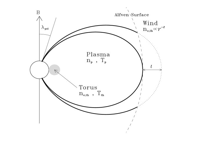
Figure 3: Section of the magnetic shell which delimits the emitting magnetospheric volume. The parameter $l$ determines the outer magnetic field line, and, consequently, the size of the radio emitting region. In the outer magnetosphere (wind zone) the density decreases with distance. Close to the star, a cooler absorbing material is present, which we ascribe to a torus of constant density $n_{\mathrm{e,th}}$ and temperature $T_{\mathrm{th}}$. The plasma temperature and density in the inner magnetosphere ($T_{\mathrm{p}}$ and $n_{\mathrm{p}}$) are discussed in Sect. 2.4. The parameter $l$ also defines also the width $\lambda_{\mathrm{pol}}$ of the polar caps, from where the wind can flow freely.

2.3 Energetic electron distribution and location of the “middle” magnetosphere

The present model assumes that electrons are accelerated in equatorial current sheets, drawn in Fig. 1 as shaded areas outside the Alfvén surface. The volume of the magnetosphere where the energetic electrons can propagate is defined in Fig. 3 by thick solid lines.

The model assumes that, in each point of the “middle” magnetosphere, the emitting electrons are isotropically distributed in pitch angle and have a power law energy distribution

$$N(\gamma)\propto N_{\mathrm{e}}(\gamma-1)^{-\delta}$$ (6)

where $\gamma$ is the Lorentz factor and $N_{\mathrm{e}}$ is the total number density of the energetic electrons. As low energy cutoff, we choose $\gamma=1.2$, corresponding to 100 keV. This choice does not influence the computation of the gyrosynchrotron emission, as discussed by Klein (klein (1987)). We choose the exponent $\delta$ considering that in the solar flares, where an acceleration process as in MCP stars is supposed, microwave and hard X-ray emission are assumed to be generated by the same population of non-thermal electrons. The spectrum of the hard X-ray photons is proportional to $\nu^{-\left(\delta+\frac{1}{2}\right)}$ when the electron population is described by Eq.(6). Since the observed hard X-ray spectrum in solar flares is a power law with an exponent ranging from $-3$ to $-4$ (Longair longair (1992)), $\delta$ should be in the range $2.5$ –$\,3.5$. At the maximum of the solar flares, i.e. close to the impulsive event, the spectrum is generally quite flat ($\delta\approx 2$ –$\,3$), and eventually it becomes steeper, as the more energetic electrons lose their energy faster. If in MCP stars the electron acceleration occurs in the current sheets outside the Alfvén radius, then the non-thermal electrons injected toward the star do not lose much energy via microwave emission, as they quickly cross the emission region (tens of seconds). Therefore they will maintain the original flat energetic spectrum. In the following, we will consider a spectrum distribution index $\delta$ in the range $2$ –$\,4$.

The electron number density remains almost constant as the electrons propagate inside the magnetosphere, as a consequence of two combined effects (Hasegawa & Sato has_e_sat (1989)): 1) particle losses due to magnetic mirroring and 2) compression due to the decreasing volume of the magnetic shell.

We assume that the number density $N_{\mathrm{e}}$ is a fraction of the thermal plasma density $n_{\mathrm{e,A}}$ at the Alfvén surface. This ratio is a free parameter in our model, since it depends on the efficiency of the acceleration process, and we assume $N_{\mathrm{e}}/n_{\mathrm{e,A}}$ in the range $10^{-4}$ –$\,1$.

The “middle” magnetosphere is defined by two magnetic lines (Fig. 3): the first is the largest closed line of the “inner” magnetosphere, tangent to the Alfvén surface in the plane of the magnetic equator; the latter is defined by the size of the current sheet, which depends on the particular physical conditions of the magnetosphere, and which we consider a free parameter of our model.

In a magnetic dipole, the equation of a field line is given by

$$r=L\cos^{2}\lambda$$

where $L$ is the distance between the center of the star and the point where the field line crosses the magnetic equatorial plane; $\lambda$ is the angle between this plane and the radius vector $r$. The middle magnetosphere is therefore identified by the points belonging to magnetic field lines having an equatorial distance $L$ between $r_{\mathrm{A}}$ and $r_{\mathrm{A}}+{l}$, where ${l}$ is a free parameter in our calculations.

Figure 4: Effective magnetic field variations (Bohlender bohl_87 (1987)) and 5 GHz lightcurves of HD 37479 and HD 37017: ($\times$) data from Drake et al. (drake_et_al (1987)), ($\bullet$) Leone & Umana (leo_e_uma (1993)), ($\diamond$) this paper.

2.4 Thermal plasma in the inner magnetosphere

The presence of thermal plasma trapped in the dead zone may affect the stellar radio emission because of the free-free absorption (André et al. andre_et_al (1988)). If its density is high enough, this plasma can partially absorb the radiation and this could result in an additional modulation of the radio lightcurve, since this effect is greater for a particular orientation of the magnetosphere. Moreover, if the density of the plasma is higher close to the star, the highest frequencies, which are emitted in the inner part of the magnetosphere, will be strongly absorbed. In contrast, the lowest frequencies, generated far from the star, are less affected by the plasma absorption. Therefore, the density distribution inside the inner magnetosphere can affect either the modulation of the radio lightcurve, or the spectrum of the source. In particular, it is important to define the extent of the absorbing matter into the inner magnetosphere, the density distribution and the temperature.

Effects of the trapped plasma have been studied at other wavelengths, as it causes also the absorption of resonance lines and of continuum when the star is seen with the equator edge-on. Smith & Groote (smith2001 (2001)), from the UV spectra of several magnetic early-B stars, found some absorbing material, which they interpreted as a “cloud” along the line of sight, characterized by a column density ($n_{\mathrm{col}}$) in the range $10^{22\,-\,23}\mathrm{\,cm}^{-2}$, temperature in the range $15\,000$ –$\,31\,000\,\mathrm{\,K}$ and average density $10^{12\,-\,13}\mathrm{\,cm}^{-3}$.

With the aim of explaining the X-ray emission from IQ~Aur, BM97 developed a magnetically confined wind-shock model, where the radiatively-driven winds from the two magnetic hemispheres collide, producing a shock that leads to an enhancement of the temperature up to $10^{6\,-\,7}$ K in the post-shock region, where X-ray radiation is emitted. They also predicted, from their X-ray model, the existence of a “disk” along the equator, made of post-shock cooling material, which could in particular explain the $15.4^{d}$ rotational modulation of $θ^1$~Ori~C seen by ROSAT (Babel & Montmerle 1997b ). In this model, the cloud observed by Smith & Groote (smith2001 (2001)) could be the inner part of the equatorial disk. Also Donati et al. (donati2001 (2001)) interpreted the X-ray emission and the variability of $β$~Cep in the framework of this model. The physical scenario of such a magnetosphere has been summarized by Montmerle (Mont (2001)) (see also Fig. 1).

Once a steady state of this process has been reached, the dynamics of the wind and the physical characteristics of the matter along lines of force of the magnetic field are ruled by the equilibrium of the total pressure. This implies that

$$n_{\mathrm{p}}k_{\mathrm{B}}T_{\mathrm{p}}=p_{\mathrm{ram}}$$ (7)

with $n_{\mathrm{p}}$ and $T_{\mathrm{p}}$ respectively the number density and the temperature of the plasma in the post-shock region and $p_{\mathrm{ram}}=\rho v^{2}$ is the ram pressure of the wind. The density $\rho$ and the speed $v$ come from Eqs.(3) and (4). If $\dot{M}=10^{-9}\leavevmode\nobreak\ M_{\sun}\mathrm{yr}^{-1}$ and $v_{\infty}=600$ km s^-1, then $p_{\mathrm{ram}}\approx 10^{-1}$ –$\,10^{-2}\mathrm{\,g\,cm^{-1}s^{-2}}$. Assuming that the radio absorbing region is the post-shock region of BM97, the previous relations give $n_{\mathrm{p}}T_{\mathrm{p}}\approx 10^{14}$ (in c.g.s.); if $T_{\mathrm{p}}\approx 10^{6}$ K, $n_{\mathrm{p}}\approx 10^{8}\mathrm{\,cm}^{-3}$.

If, in addition, the post-shock region were also responsible for the absorption of the UV lines and continuum (Smith & Groote, smith2001 (2001)), a column density of $10^{22}\mathrm{\,cm}^{-2}$ should lead to a characteristic size of the post-shock region given by $n_{\mathrm{col}}/n_{\mathrm{p}}$ that, considering the Eq.(7), is $\approx 10^{22}/n_{\mathrm{p}}\approx 10^{8}T_{\mathrm{p}}$. Therefore, to be responsible also for the absorption of both UV features and radio radiation, the X-ray emitting region (with $T_{\mathrm{p}}\approx 10^{6}$ K) should be very large ($>10^{14}\mathrm{\,cm}$), at least some hundreds times the stellar radius or some tens the Alfvén radius. In few words, so high a column density cannot be reached inside the Alfvén radius unless the density is very high.

The other possibility is that the X-ray emitting region (BM97) is not responsible for the UV absorptions, and the only valid relation between $T_{\mathrm{p}}$ and $n_{\mathrm{p}}$ is Eq.(7). If $T_{\mathrm{p}}\approx 10^{6\,-\,7}$ K, we find $n_{\mathrm{p}}\approx 10^{8\,-\,7}\mathrm{\,cm^{-3}}$. Briefly, starting from the stellar surface, we have:

• a dense region ($n_{\mathrm{e,th}}\approx 10^{12}\mathrm{\,cm}^{-3}$) at stellar temperature, ($T_{\mathrm{th}}\approx T_{\mathrm{eff}}$) with a size of about $10^{11}$ cm, less than the stellar radius: this region is responsible for the UV absorption; for simplicity, a torus shape has been assumed to account for the two equatorial matter distributions, with density $n_{\mathrm{e,th}}$ and temperature $T_{\mathrm{th}}$ assumed constant;

• a less dense region ($n_{\mathrm{p}}\approx 10^{7\,-\,8}\mathrm{\,cm}^{-3}$) at high temperature ($T_{\mathrm{p}}\approx 10^{6\,-\,7}$ K), whose maximum extent is defined by the magnetic confinement ($B^{2}/8\pi\approx n_{\mathrm{p}}kT_{\mathrm{p}}$). Since the magnetic field is given by Eq.(5), the maximum size is given by

  $$L=\left(\frac{B_{\mathrm{p}}^{2}}{16\pi n_{\mathrm{p}}k_{\mathrm{B}}T_{\mathrm{p}}}\right)^{1/6}$$

  which gives $L=23$ –$\,18\,R_{\ast}$ respectively for $B_{\mathrm{p}}=10\,000$ –$\,5\,000$ Gauss. In any case $L$ is greater than the Alfvén radius (Fig. 2, lower panel). We can therefore assume that this region fills all the inner magnetosphere.

Figure 3 also outlines this scenario. The actual situation can, however, be a little different since the above picture is valid in the hypothesis of a non-rotating star. In fact, BM97 showed that the temperature of the plasma in the inner magnetosphere remains almost constant if the star does not rotate, but can increase linearly outward in the case of a fast rotation (with the dipole axis aligned with the rotational one, i.e with $\beta=0$). Since the plasma is in pressure equilibrium with the wind ram pressure, we have to add to the first term of Eq.(7) a kinetic term that accounts for the rotational energy, in a similar way as in Eq.(2). In any case, if the rotation is considered, the density should decrease outward. In the case that $\beta\neq 0$ the situation is more complex, but when $\beta\approx 90\degr$ the rotational axis lies close to the magnetic equatorial plane, and the regions close to the rotational axis can be considered to be not rotating, while other regions can be rotating fast; the result is intermediate between a non-rotating and a rotating magnetosphere.

The presence of thermal plasma has been considered in the calculation of the emitted radiation (see Appendix B.1), including free-free thermal emission and absorption (Dulk dulk (1985)) as well as the Razin effect.

Table 1: Stellar parameters

Measured parameters
	$D$	$P_{\mathrm{rot}}$	$B_{\mathrm{p}}$	$i\degr$	$\beta\degr$
	[pc]	[day]	[Gauss]
HD 37479	$352^{{\dagger}}$	$1.19081^{a}$	$6800^{a}$	$72^{b}$	$56^{b}$
HD 37017	$373^{{\dagger}}$	$0.901195^{a}$	$7700^{a}$	$25^{b}$	$65^{b}$
Derived parameters
	$r_{\mathrm{A}}$ (min–max)		$n_{\mathrm{e,A}}$ (min–max)
	[$R_{\ast}$]		[$\times 10^{6}$ cm-3]
HD 37479	13.18–15.75		2.6–3.7
HD 37017	12.59–16.36		2.4–4.1

• Hipparcos main catalogue

• Bohlender et al. (bohl_87 (1987))

• Shore & Brown (sho_e_bro (1990))

3 Application to HD 37479 and HD 37017

The model developed in this paper has been used to simulate the radio lightcurves of two MCP stars: HD 37479 (=$\sigma$ Ori E) and HD 37017.

Figure 5: HD 37017: examples of search of solutions. Light curve characteristics: maximum flux density (top panels) and ratio $\Delta$ (lower panels) as a function of the magnetic shell thickness $l$ normalized to the stellar Alfvèn radius $r_{A}$. In these examples, the spectral index of the relativistic electrons ($\delta$) has been fixed to 2, and the temperature of the plasma at the base of the inner magnetosphere ($T_{\mathrm{p}}$) to $10^{5}$ K. The rotation of the star has been considered. From left to right: solutions for increasing values of the plasma density ($n_{\mathrm{p}}$) at the base of the inner magnetosphere. In each pair of panels, $S_{\mathrm{max}}$ and $\Delta$ are computed for different number density of the emitting electrons ($N_{\mathrm{r}}$) as percentage of the number density of thermal plasma at the Alfvén point $n_{\mathrm{e,A}}$ (different line styles). A valid solution is given if the computed $S_{\mathrm{max}}$ and $\Delta$ are within the observed values (shaded areas) for the same value of $l/r_{\mathrm{A}}$. The good solution is indicated by a vertical line and two squares.

The 5 GHz emission of these two stars appears to vary with the rotational period. Fig. 4 shows the effective magnetic field $B_{\mathrm{e}}$ and the observed 5 GHz flux densities $S_{5}$ as reported by Leone & Umana (leo_e_uma (1993)). We add to these data the new results of two VLA observations: HD 37479 was observed on 29 April 1995 (21:29–21:47 UT) and HD 37017 on 29 May 1995 (18:42–19:06 UT). We reduced and analysed the data following the procedures used by Leone & Umana (leo_e_uma (1993)). We measured as flux densities respectively $3.0\pm 0.1$ mJy at phase $\Phi=0.545$ and $1.9\pm 0.2$ mJy at $\Phi=0.16$, with rotational phases computed by using the ephemeris determined by Bohlender et al. (bohl_87 (1987)). Those data are reported in Fig. 4 as diamonds symbols. Leone & Umana (leo_e_uma (1993)) noted that, while the radio data of HD 37017 can be fitted by a single sinusoidal like curve, for HD 37479 the radio variation can have a double-wave behaviour, as for the variations of the helium abundance in those stars. They argued that the radio emission is probably related to $|B_{\mathrm{e}}|$, with the minimum corresponding approximately with the zero of the longitudinal magnetic field.

Regarding the X-ray emission, that could arise from the inner magnetosphere, both stars have been observed in the ROSAT all-sky survey (Berghöfer et al. RASS (1996)). While HD 37017 is reported as a non-detection ($\lg L_{\mathrm{X}}<30.7$), HD 37479 is a doubtful detection (Drake et al. drake1994 (1994)) since it is a visual binary with a hotter primary component closer than $1\arcmin$, likely the predominant contributor to the observed X-ray emission.

To simulate the 5 GHz radio emission of these two MCP stars, we fix a stellar radius of $R_{\ast}=4\leavevmode\nobreak\ R_{\sun}$ (Shore & Brown sho_e_bro (1990)) and an effective temperature $T_{\mathrm{eff}}=24\,000$ K (Leone leone (1991)). The other physical stellar parameters are reported in Table 1. We set the mass loss rate and the terminal wind speed respectively to $\dot{M}=10^{-9}\leavevmode\nobreak\ M_{\sun}\mathrm{yr}^{-1}$ and $v_{\infty}=600$ km s^-1, according to Drake et al. (drake_et_al (1987)). The above mass loss rates are not the actual values, but refer to the case of a spherical wind. In fact, the wind is confined by the magnetosphere, leading to the formation of the torus as discussed in Sect. 2.4, and it can escape only from the two polar caps defined by the largest closed field line (see Sect. 2.2 and Fig. 3). Using these observing constraints we can univocally define the equatorial radius of the Alfvén surface and the local thermal plasma densities. The maximum and minimum equatorial Alfvén radius ($r_{\mathrm{A}}$) and the corresponding thermal electron number density ($n_{\mathrm{e,A}}$) for HD 37479 and HD 37017 are also reported in Table 1. The actual mass loss rate $\dot{M}_{\mathrm{act}}$ is computed considering that the polar caps have an aperture $\lambda_{\mathrm{pol}}$ defined by the intersection between the stellar surface and the magnetic field line that identifies the “outer” magnetosphere (see Fig. 3). Using the above stellar wind parameters, we get $\lambda_{\mathrm{pol}}\approx 15\degr$, so that the area of the two caps is only $2\%$ of the total surface, giving $\dot{M}_{\mathrm{act}}\approx 10^{-11}M_{\sun}\mathrm{yr}^{-1}$.

The aim of our analysis is to derive possible configurations of the magnetosphere, represented by the free parameters of the model ($l$, $N_{\mathrm{e}}$, $\delta$, $T_{\mathrm{p}}$ and $n_{\mathrm{p}}$), which result in simulated lightcurves at 5 GHz able to reproduce the observations. The search of these combinations of the free parameters, computing the radio flux at different values of the rotational phase, could be very time-consuming so, to restrict the computing time, we simulate the flux density of the two stars only for particular stellar orientations, coinciding with the extremes and the nulls of the magnetic field curve. The characteristic of the observed radio lightcurves may be summarized by the maximum flux density $S_{\mathrm{max}}$ and the ratio $\Delta=S_{\mathrm{min}}/S_{\mathrm{max}}$, that expresses the depth of the modulation, being minimum for high modulation.

The lightcurve characteristics derived by fitting the observing data for HD 37479 and HD 37017 are, respectively:
$S_{\mathrm{max}}=4.0\pm 0.2$ mJy, $\Delta=0.65\pm 0.06$ and
$S_{\mathrm{max}}=2.6\pm 0.1$ mJy, $\Delta=0.58\pm 0.04$.

Table 2: With and without rotational effects, the 5 GHz radio lightcurves of HD 37479 and HD 37017 are reproduced for the listed values of: spectral index of non-thermal electron energy distribution ($\delta$); temperature ($T_{\mathrm{p}}$) and thermal electron density ($n_{\mathrm{p}}$) of the plasma in the post-shock region as extrapolated to the stellar surface; equatorial thickness in Alfvén radius units ($l/r_{\mathrm{A}}$); and total number density of non-thermal electrons ($N_{\mathrm{r}}$). The asterisk in the last column indicates the possible solutions that reproduce the almost flat observed spectral index.

Star	Rotation	$\delta$	$T_{\mathrm{p}}$[K]	$n_{\mathrm{p}}$[cm-3]	$l/r_{\mathrm{A}}$	$N_{\mathrm{r}}$[cm-3]	Spectral index
HD 37479	No	2	$1.0\times 10^{5}$	$>1.0\times 10^{9}$	0.74	$6.3\times 10^{2}$	–0.40 – 0.10
	Yes	2	$1.0\times 10^{5}$	$1.0\times 10^{9}$	0.05	$3.1\times 10^{3}$	–0.18 – 0.31
	Yes	2	$1.0\times 10^{5}$	$2.0\times 10^{9}$	0.40	$6.3\times 10^{2}$	–0.10 – 0.34	$\ast$
	Yes	2	$1.0\times 10^{5}$	$3.0\times 10^{9}$	0.83	$4.5\times 10^{2}$	–0.07 – 0.21	$\ast$
	Yes	3	$1.0\times 10^{5}$	$1.0\times 10^{9}$	0.11	$3.1\times 10^{4}$	–0.07 – 0.61
	Yes	3	$1.0\times 10^{5}$	$2.0\times 10^{9}$	0.77	$9.4\times 10^{3}$	–0.04 – 0.56
	Yes	4	$1.0\times 10^{5}$	$1.0\times 10^{9}$	0.27	$3.1\times 10^{5}$	0.05 – 0.74
	Yes	4	$1.0\times 10^{5}$	$2.0\times 10^{9}$	1.05	$1.5\times 10^{5}$	0.11 – 0.69
	No	2	$1.0\times 10^{6}$	$5.0\times 10^{8}$	0.36	$9.4\times 10^{2}$	0.12 – 0.75
	No	2	$1.0\times 10^{6}$	$1.0\times 10^{9}$	0.74	$6.3\times 10^{2}$	0.09 – 0.54
	No	3	$1.0\times 10^{6}$	$3.0\times 10^{8}$	0.18	$3.1\times 10^{4}$	0.06 – 0.87
	No	3	$1.0\times 10^{6}$	$4.0\times 10^{8}$	0.56	$1.5\times 10^{4}$	0.09 – 0.92
	No	3	$1.0\times 10^{6}$	$5.0\times 10^{8}$	0.91	$1.2\times 10^{4}$	0.12 – 0.99
	No	4	$1.0\times 10^{6}$	$1.0\times 10^{8}$	0.12	$7.8\times 10^{5}$	0.02 – 0.81
	No	4	$1.0\times 10^{6}$	$2.0\times 10^{8}$	0.12	$7.8\times 10^{5}$	0.11 – 0.93
	No	4	$1.0\times 10^{6}$	$3.0\times 10^{8}$	0.45	$3.1\times 10^{5}$	0.16 – 0.96
	No	4	$1.0\times 10^{6}$	$4.0\times 10^{8}$	0.83	$2.2\times 10^{5}$	0.21 – 1.05
	Yes	4	$1.0\times 10^{6}$	$1.0\times 10^{8}$	0.05	$1.5\times 10^{6}$	–0.09 – 0.58
	Yes	4	$1.0\times 10^{6}$	$1.0\times 10^{9}$	0.05	$1.5\times 10^{6}$	–0.09 – 0.60
	No	4	$1.0\times 10^{7}$	$1.0\times 10^{7}$	0.07	$1.5\times 10^{6}$	–0.04 – 0.71
	No	4	$1.0\times 10^{7}$	$1.0\times 10^{8}$	0.07	$1.5\times 10^{6}$	–0.04 – 0.71
	Yes	4	$1.0\times 10^{7}$	$>1.0\times 10^{7}$	0.09	$7.8\times 10^{5}$	–0.11 – 0.66
HD 37017	No	2	$1.0\times 10^{5}$	$>1.0\times 10^{9}$	0.59	$4.5\times 10^{2}$	–0.44 – 0.09
	Yes	2	$1.0\times 10^{5}$	$3.0\times 10^{9}$	0.53	$3.1\times 10^{2}$	0.00 – 0.34	$\ast$
	Yes	3	$1.0\times 10^{5}$	$2.0\times 10^{9}$	0.62	$4.7\times 10^{3}$	0.14 – 0.68
	Yes	4	$1.0\times 10^{5}$	$2.0\times 10^{9}$	0.67	$9.0\times 10^{4}$	0.08 – 0.86
	No	2	$1.0\times 10^{6}$	$5.0\times 10^{8}$	0.05	$3.1\times 10^{3}$	0.27 – 1.10
	No	2	$1.0\times 10^{6}$	$1.0\times 10^{9}$	0.59	$4.5\times 10^{2}$	0.22 – 0.60
	No	3	$1.0\times 10^{6}$	$4.0\times 10^{8}$	0.40	$9.4\times 10^{3}$	0.29 – 1.18
	No	4	$1.0\times 10^{6}$	$3.0\times 10^{8}$	0.36	$1.5\times 10^{5}$	0.29 – 1.12

The simulations for the two stars are performed by using different combinations of the free parameters of the model:

• $l$: equatorial thickness of the magnetic shell (Fig. 3), such that $l/r_{\mathrm{A}}=0.025$ – 1;
  

• $N_{\mathrm{e}}$: total number density of the non-thermal electrons, in the range $10^{2}$ –$\,10^{6}$cm^-3, with $N_{\mathrm{e}}<n_{\mathrm{e,A}}$;
  

• $\delta$: spectral index of the non-thermal electron energy distribution (Eq.(6)), in the range 2 – 4;
  

• $T_{\mathrm{p}}$ and $n_{\mathrm{p}}$: temperature and number density of the plasma in the inner magnetosphere (the post-shock region of BM97); they are chosen so that $T_{\mathrm{p}}n_{\mathrm{p}}=p_{\mathrm{ram}}/k_{\mathrm{B}}$ is in the range $10^{14}$ – $10^{15}$ (in c.g.s.), with $T_{\mathrm{p}}=10^{5}$ – $10^{7}$ and $n_{\mathrm{p}}=10^{7}$ – $10^{10}$cm^-3;
  

• rotation: if the star does not rotate, the thermal plasma density is considered constant within the inner magnetosphere; if, on the contrary, we consider the rotation, the thermal plasma density decreases linearly outward, while the temperature increases. $T_{\mathrm{p}}$ and $n_{\mathrm{p}}$ are considered as the values at $r=R_{\ast}$.
  

The behaviour of $S_{\mathrm{max}}$ and $\Delta$ versus the magnetic shell thickness $l$ is investigated for models computed assuming different values of $N_{\mathrm{e}}$, $\delta$, $T_{\mathrm{p}}$, $n_{\mathrm{p}}$, and rotation. Fig. 5 shows some examples of the adopted method of searching for good combinations of the free parameters. The shaded areas represent the observed values of $S_{\mathrm{max}}$ and $\Delta$ derived from the observed 5 GHz lightcurves. For each value of $N_{\mathrm{e}}$, the good solutions must show the observed values of $S_{\mathrm{max}}$ and $\Delta$ for the same value of $l/r_{\mathrm{r}}$. They are reported in Table 2 for the two stars.

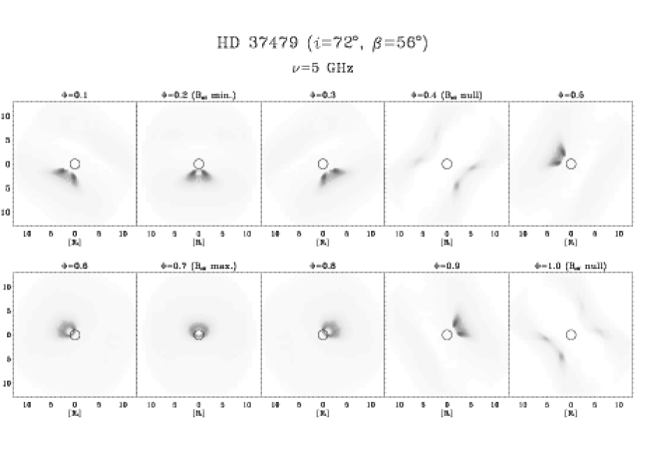
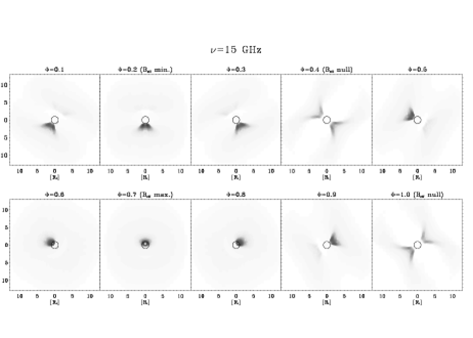
Figure 6: Simulated brightness distribution of HD 37479 at $\nu=5$ GHz and $\nu=15$ GHz for different values of rotational phase. Stellar orientations corresponding to the extremes and the null effective magnetic field are indicated.

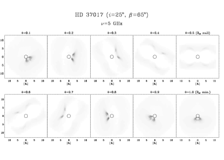
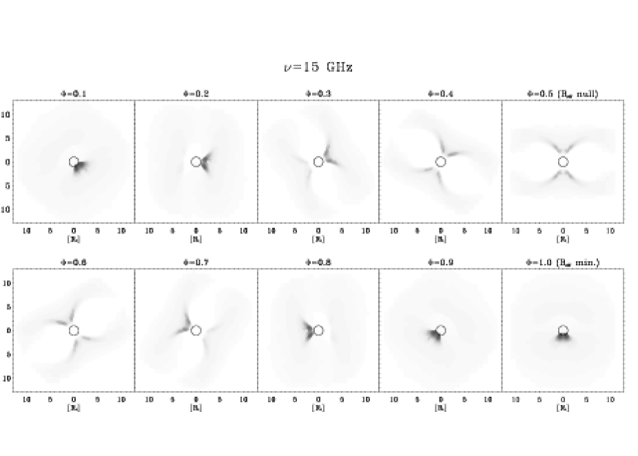
Figure 7: As Fig. 6 for HD 37071.

4 Discussion

The model presented in this paper is used to test the scenario proposed to explain the origin of radio emission from MCP stars and, if possible, to derive quantitative information about the physical conditions of their magnetospheres.

First, the characteristic quantities $S_{\mathrm{max}}$ and $\Delta$ of the lightcurves at 5 GHz of HD 37479 and HD 37017 are computed for different combinations of $l$, $N_{\mathrm{e}}$, $\delta$, $T_{\mathrm{p}}$, $n_{\mathrm{p}}$, including also the different behaviour of the thermal plasma in the inner magnetosphere as the star rotates or not. All the possible solutions are shown in Table 2.

Second, for any possible solution, we compute the emerging radio flux also at 8.4 and 15 GHz; the spectral index of the simulated spectra must be flat (say in the range –0.1 – 0.4) as reported by Drake et al. (drake_et_al (1987)) and Leone et al. (leo96 (1994)). The solutions with the required spectral index are indicated by an asterisk in the last column of Table 2.
The model is not computed at 1.4 and 22 GHz because:
1) at low frequency the emitting region extends far from the star and close to the Alfvén surface, where the geometry of the magnetosphere is not yet well known, and
2) at high frequency the magnetosphere must be so closely sampled that computational times are prohibitive.

Third, we compute the radio lightcurves at 8.4 and 15 GHz with the aim of predicting the behaviour of our model, which should be tested in the future with multi-frequency observations.

4.1 Effect of the rotation

The radio lightcurves at 5 GHz for the two stars can be reproduced by several combinations of free parameters. Particularly, the effects of the rotation seem to be important.

Neglecting the effects of rotation, i.e. assuming that the density and the temperature of the inner magnetosphere are constant, we find that $T_{\mathrm{p}}=10^{5}$ K, the electron energy spectrum must be hard ($\delta=2$) and a small relativistic electron number $N_{\mathrm{e}}$ is required to reproduce the observed radio emission. In this case $n_{\mathrm{p}}$ must be quite high ($>1\times 10^{9}\mathrm{\,cm}^{-3}$), in order to have the observed modulation of the radio lightcurve. Also if $T_{\mathrm{p}}=10^{6}$ K we get solutions for both stars, for $\delta=2,3,4$; $N_{\mathrm{e}}$ increases as the electron energy spectrum becomes softer ($\delta=4$), reaching almost the number density of the Alfvén point (i.e. $\approx 10^{6}\mathrm{\,cm}^{-3}$). $n_{\mathrm{p}}$ is lower than in the previous case, being in the range $10^{8}$ – $10^{9}\mathrm{\,cm}^{-3}$.
For $T_{\mathrm{p}}=10^{7}$ K, only the behaviour of HD 37479 can be reproduced, but only for $\delta=4$ and very high values of $N_{\mathrm{e}}$.

The situation is different if the rotation has been taken into account, considering that $T_{\mathrm{p}}$ increases linearly outward and $n_{\mathrm{p}}$ decreases according to the relation $T_{\mathrm{p}}n_{\mathrm{p}}=const$. In Table 2 their values extrapolated at $R=R_{\ast}$ are reported.
For $T_{\mathrm{p}}=10^{5}$ and $\delta=2,3,4$, the lightcurves of both stars are well reproduced. The number density at the base of the inner magnetosphere is about $10^{9}\mathrm{\,cm}^{-3}$.
For $T_{\mathrm{p}}=10^{6}$ K we get solutions only for HD 37479, only with $\delta=4$ but with $N_{\mathrm{e}}\approx n_{\mathrm{e,A}}$.
Simulations at $T_{\mathrm{p}}=10^{7}$ K do not show any possibility for HD 37017, while for HD 37479 they are limited to $\delta=4$ and very high $N_{\mathrm{e}}$.

Figure 8: Top panel: Observed spectrum of HD 37479 by Leone et al. (leo96 (1994)) ($\bullet$) and its linear 2 – 15 GHz fit (dotted lines) are compared with the computed spectra at minimum and maximum radio emission for the two solutions marked with asterisks in Table 2. In the order they are listed, dashed and dashed-dotted lines represent these solutions.
Bottom panel: with the previous symbols, the observed spectrum of HD 37017 is compared with the only solution found.

Figure 9: Left panels: comparison of the observed 5 GHz data of Fig. 4 and the computed lightcurves corresponding with the accepted solutions of Table 2. Central and right panels: lightcurves at 8.4 and 15 GHz as predicted by the model. See Fig. 4 for the meaning of the symbols.

4.2 The effect of the electron energy spectrum

As already noted, a hard non-thermal electron energy population, such as $\delta=2$, is able to reproduce the observed radio emission with small $N_{\mathrm{e}}$ ($\approx 10^{2}$ – $10^{3}\mathrm{\,cm}^{-3}$). A softer population, say $\delta=4$, even if able to reproduce the emission, requires a very efficient acceleration process, as almost all the electrons flowing with the stellar wind should be accelerated up to relativistic energies.
Our results indicate that a hard electron energy population is more probable.

4.3 Simulation of radio lightcurves and spectra

In order to get the spectral index, radio fluxes at 8.4 and 15 GHz are computed for any solution at maximum and minimum lightcurve. The range of variation of the spectral index is also reported in Table 2. Only two solutions for HD 37479 and one for HD 37017 give spectral indices similar to the observed ones. They have in all cases a quite hard electron energy distribution ($\delta=2$) and are all consistent with a rotating magnetosphere, where the density of the absorbing matter in the inner magnetosphere decreases outward quite linearly, while the temperature increases. Radio spectra at maximum and minimum flux are shown in Fig. 8 for the accepted solutions, together with the spectral data from Leone et al. (leone_et_al (1994)). There is a good agreement, and this result encourages us to extend the model at lower and higher frequency.

The simulated radio lightcurves for HD 37479 and HD 37017, corresponding to the three accepted solutions, are shown in Fig. 9. In the left panels, the 5 GHz simulations are superimposed on the measurements from the literature. For the first star, there is no significant difference between the two simulated radio lightcurves and it is, therefore, impossible to discriminate between them by using only single frequency data. Even though radio lightcurves are not available for those two stars at other frequencies, we computed the synthetic curves at 8.4 and 15 GHz in order to give a prediction of the behaviour in a wide range of frequency. The comparison between the results of our model computed with multifrequency observations is therefore crucial.

Both stars are unfortunately too far away (Table 1) to give us the opportunity to resolve the radio sources by using Very Long Baseline Interferometry (VLBI). In fact, at 5 GHz, the extent of the radio emitting region (Fig. 6) is about 10 stellar radii, corresponding to an angular size of about 1.5 milliarcseconds (mas). The angular resolution of the VLBI arrays (with a maximum baseline of about 8000 km) is 1.5 mas, and the source cannot resolved. This is in agreement with the results of Phillips & Lestrade et al. (phill (1988)) who did not resolve HD 37479 with high-sensitivity intercontinental VLBI. At 15 GHz the resolution of the VLBI is 0.5 mas and the sources can be only barely resolved if observed at a rotational phase corresponding to the zero of longitudinal magnetic field $B_{\mathrm{e}}$, when the radio source has its maximum angular extent (a little less than 10 stellar radii). A closer MCP star should be observed in VLBI in order to test the morphology predicted by our model.

4.4 X-ray emission

The physical conditions of the inner magnetosphere play an important role in the emerging radio flux because of the free-free absorption by plasma. The inner magnetosphere is modelled following the magnetically wind-shock model by BM97. By performing more than 56 000 simulations per star, changing all the free parameters of our model, we find only 3 solutions satisfying all the observational constraints. All 3 solutions indicate that the effects of rotation are not negligible. For the two stars, we find that the temperature increases outward from about $10^{5}$ to $1.4\times 10^{6}$ K, while the density decreases from $2-3\times 10^{9}$ to $2\times 10^{8}\mathrm{\,cm^{-3}}$. As a by-product of our model, we can estimate the X-ray emission of the inner magnetosphere once its configuration has been found according to the radio emission model. Following a procedure similar to that used for the computation of the radio flux, we compute for each element of the magnetosphere the temperature and the number density in order to get the Bremsstrahlung emission coefficients for a thermal plasma. The emitted power is then integrated in the range of energy $0.1-2.0$ KeV, and the resulting X-ray luminosities are evaluated as $\lg L_{\mathrm{X}}=30.06$ for HD 37479 and $\lg L_{\mathrm{X}}=30.42$ for HD 37017. These values are consistent with the limits of detection of the ROSAT all-sky survey, as in Sect. 3. However, with the new X-ray telescopes now available (Chandra and XMM), both stars should be easily detectable. In fact, the corresponding fluxes at the Earth would be respectively $1.2\times 10^{-13}$ and $2.4\times 10^{-13}\mathrm{\,erg\,s^{-1}\,cm^{-2}}$, and the detection limits for a point source for the two instruments are $10^{-15}\mathrm{\,erg\,s^{-1}\,cm^{-2}}$ in a few 10 Ksec.

Recently, Schulz et al. (schulz (2003)) found that the X-ray emission from the MCP-like O7V star $θ^1$~Ori~C (Donati et al. donati2002 (2002)) revealed by Chandra is consistent with a magnetically confined wind. Unfortunately, radio observations of this object cannot be used to test our model as this star is embedded in the Orion nebula, one of the brightest radio sources.

The capability to reproduce also the X-ray emission represents an independent and further confirmation of the validity of our model. Multi-wavelength radio observations in conjunction with X-ray observations will be a real test for our model.

5 Conclusion

The study of radio emission from the MCP stars and, in particular, the analysis of the observed modulations offer a unique opportunity to determine the physical properties of the stellar magnetosphere.

The numerical model developed in this paper is used to reproduce the 5 GHz radio lightcurves of two well known MCP stars: HD 37479 and HD 37017.

The capability of our numerical model to give us an estimation of the physical condition of the magnetosphere is limited by the lack of multifrequency radio lightcurves. However, the spectral information available up to now allows us to focus on a small range of possible solutions, all of them indicating a hard energetic population of non-thermal-emitting electrons, and an inner magnetosphere filled by a thermal plasma consistent with a wind-shock model that provides also X-ray emission.

The possibility to test the radio curves at more than one frequency would allow us to put more stringent constraints on the model.

Our simulations provide useful information that may be summarized as follows:

• we confirm the qualitative model proposed by several authors to explain the origin of non-thermal electrons as responsible for the observed radio emission from MCP stars;
  

• we point out the importance of the thermal electrons trapped in the inner magnetosphere for reproducing the rotational modulation of the measured radio flux density and the radio spectra of the MCP; this plasma can prroduce X-ray emission;
  

• the length of the current sheets, where the electrons are accelerated up to relativistic energies, is about one half of the Alfvén radius; the acceleration process has an efficiency of about $10^{-4}$, as only this small fraction of the electrons in the current sheets is accelerated ; those non thermal electrons have an hard energetic spectrum ($N(\gamma)\propto(\gamma-1)^{-\delta}$), with $\delta\approx 2$; the inner magnetosphere is filled by thermal plasma, whose temperature increases outward from $10^{5}$ up to $10^{6}$ K, consistent with a rotating magnetosphere.

We emphasize the importance of multifrequency radio lightcurves and contemporaneous X-ray observations for a further test our model. This will be a powerful investigation tool for studying the physics of the stellar magnetosphere.

Appendix A

A.1 Procedures

We numerically developed the physical scenario proposed to explain the origin of radio emission arising from the magnetosphere of MCP stars. The aim is to reproduce the centimetric radio emission as a function of the rotational phase.

For any rotational phase and a given wavelength, the procedure is:

• 3D sampling of the magnetosphere and calculation of the magnetic field vector $\@vec{B}$;

• definition of the Alfvén radius and of inner, middle and outer magnetosphere;

• calculation of the number density $n_{\mathrm{e}}$ of the non-thermal electrons in each point of the grid;

• calculation of emission and absorption coefficients;

• integration of the transfer equation along paths parallel to the line of sight;

• brightness distribution in the plane of the sky, total flux emitted toward the Earth.

A.2 The reference frame

In the oblique rotator model the magnetic axis has an obliquity $\beta$ with respect to the rotational axis $\@vec{\Omega}$, which in turn forms an angle $i$ with respect to the line of sight. Thus the orientation of the magnetosphere changes with respect to the line of sight as a function of the rotational phase $\Phi$. For the purpose of the model, the most convenient reference frame where to sample the magnetosphere is the fixed frame $Ox^{\prime}y^{\prime}z^{\prime}$, with origin $O$ at the center of the star, axis $x^{\prime}$ direct toward the Earth, axes $y^{\prime}$ and $z^{\prime}$ in the plane of the sky with $z^{\prime}$ coinciding with the projection of $\@vec{\Omega}$ on the plane of the sky. However, since a dipole has an axial symmetry, the most convenient reference frame to compute the vector $\@vec{B}$ and all the other physical parameters is the frame $Oxyz$, anchored to the star, having axis $z$ coinciding with the axis of the dipole. Here the axis $x$ lies in the plane defined by the rotational and dipole axes. In this frame, the components of vector $\@vec{B}$ are:

$$B_{x}=3m\frac{xz}{r^{5}}$$

$$B_{y}=3m\frac{yz}{r^{5}}$$ (8)

$$B_{z}=m\left(3\frac{{z}^{2}}{r^{5}}-\frac{1}{r^{3}}\right)$$

with $m$ the magnetic momentum ($m=\frac{1}{2}B_{\mathrm{p}}R_{\ast}$). If we indicate by ${\bf\Re}(\Phi)$ the transformation matrix to pass from the frame $Oxyz$ to $Ox^{\prime}y^{\prime}z^{\prime}$, the magnetic field vector in $Ox^{\prime}y^{\prime}z^{\prime}$ is given by:

$${\@vec{B}}^{\prime}({\@vec{r}}^{\prime})=\Re\@vec{B}(\Re^{-1}{\@vec{r}}^{\prime}).$$ (9)

A.3 Rotation of the magnetosphere

All the physical quantities of the magnetosphere, either vectorial or scalar, are easily computable in the stellar reference frame $Oxyz$. However, we need to know them in the reference frame $Ox^{\prime}y^{\prime}z^{\prime}$ of the observer. For this purpose, we need to know the transformation matrix $\Re$ of Eq.(9).

The stellar observing system $Oxyz$ is defined by the direction of the magnetic axis ($z$ axis), and the intersection between the plane of the magnetic equator and the plane where the $z$ axis and the rotational axis $\Omega$ lie (Fig. 10a).

In the observing reference frame $Ox^{\prime}y^{\prime}z^{\prime}$ the stellar orientation is univocally defined by the inclination $i$ of the rotation axis with respect to the line of sight, the misalignment $\beta$ of the magnetic axis with respect to the rotation axis $\Omega$ and the angle $\Phi$ corresponding to the rotational phase. The three angles $i$, $\beta$ and $\Phi$ define the transformation matrix $\Re(i,\beta,\Phi)$ between $Oxyz$ and $Ox^{\prime}y^{\prime}z^{\prime}$.

The matrix $\Re$ is the result of three space rotations:

• $$\Re_{1}=\left(\begin{array}[]{ccc}\cos\beta&0&-\sin\beta\\ 0&1&0\\ \sin\beta&0&\cos\beta\end{array}\right)$$

  rotation of an angle $\beta$ around the $y$ axis (Fig. 10 a-b) so that $z\rightarrow z_{1}$ coincides with the rotation axis $\Omega$;
  

• $$\Re_{2}=\left(\begin{array}[]{ccc}\cos\Phi&-\sin\Phi&0\\ \sin\Phi&\cos\Phi&0\\ 0&0&1\end{array}\right)$$

  rotation of an angle $-\Phi$ around $\Omega$ (Fig. 10 c-d) so that $x_{1}\rightarrow x_{2}$ lies in the plane defined by the line of sight and $\Omega$;
  

• $$\Re_{3}=\left(\begin{array}[]{ccc}\sin i&0&\cos i\\ 0&1&0\\ -\cos i&0&\sin i\end{array}\right)$$

  rotation of $(\pi/2-i)$ around $y_{2}$ axis (Fig. 10 e-f) so that $x_{2}\rightarrow x_{3}$ coincides with the line of sight (axis $x^{\prime}$).

The transformation matrix $\Re$ can so be defined as:

$$\Re=\Re_{3}\Re_{2}\Re_{1}$$

The inverse transformation, from $Ox^{\prime}y^{\prime}z^{\prime}$ to $Oxyz$, is then defined by the three inverse rotations:

$$\Re^{-1}={\Re_{1}}^{-1}{\Re_{2}}^{-1}{\Re_{3}}^{-1}$$

Rotation matrices are unitary, so the inverse rotations are described by the transposed matrices.

Figure 10: Three rotations permit to pass from the stellar reference frame $Oxyz$ (panel a) to that of the observer $Ox^{\prime}y^{\prime}z^{\prime}$ (panel f).

Appendix B

B.1 The gyrosynchrotron emission

To calculate the total flux density radiated by the magnetosphere, the equation of radiative transfer was numerically integrated, independently for the ordinary and extraordinary modes of propagation, along the axis $x^{\prime}$.

For the gyrosynchrotron emission and absorption coefficients $\eta_{\nu}$ and $k_{\nu}$, the approximate expressions given by Klein (klein (1987)) were used if the harmonic of gyrofrequency was bigger then 4; otherwise the general expressions given by Ramaty (ramaty (1969)) have been adopted.

The presence of the star was taken into account by putting at the center of the grid a sphere of radius equal to the stellar radius ($R_{\ast}$), and opaque to the radiation.

Defining $i,j$ and $k$ as the index over $x^{\prime}$, $y^{\prime}$ and $z^{\prime}$, the method used to integrate the equation of radiative transfer may be summarized as follows:

• calculation of the specific intensity inside each cube element of geometrical depth $\Delta l$:

  $$\Delta I_{\nu}(i,j,k)=\frac{\eta_{\nu}(i,j,k)}{k_{\nu}(i,j,k)}\left[1-e^{-k_{\nu}(i,j,k)\Delta l}\right]$$

• calculation of the optical depth of the column matter between each grid element and the Earth:

  $$\tau_{\nu}(i,j,k)=\sum_{i^{\prime}=i+1}^{N}k_{\nu}(i^{\prime},j,k)\Delta l$$

• calculation of the specific intensity $I_{\nu}$ arising from each direction parallel to line of sight:

  $$I_{\nu}(j,k)=\sum_{i}\Delta I_{\nu}(i,j,k)e^{-\tau_{\nu}(i,j,k)}.$$

Each element of matrix $I_{\nu}(j,k)$ represents the specific intensity in the plane of the sky.

The total flux density can be derived using the relation:

$$S_{\nu}=\frac{1}{D^{2}}\sum_{j}\sum_{k}I_{\nu}(j,k)\Delta l^{2}$$

where $D$ is the distance of the source.

References

- (1) André, P., Montmerle, T., Feigelson, E.D., Stine, P.C. & Klein K.L. 1988, ApJ, 335, 940
- (2) Babcock, H.W., 1949, Observatory 69, 191
- (3) Babel, J., & Montmerle T. 1997a, A&A, 323, 121 (BM97)
- (4) Babel, J., & Montmerle T. 1997b, ApJL, 485, 29
- (5) Berghöfer, T.W., Schmitt, J.H.M.M., & Cassinelli J.P. 1996, A&AS, 118, 481
- (6) Bohlender, D.A., Brown, D.N., Landstreet, J.D., & Thompson, I.B. 1987, ApJ, 323, 325
- (7) Castor, J.I., & Simon, T. 1983, ApJ, 265, 304
- (8) Donati, J.-F., Wade, G.A., Babel, J., et al. 2001, MNRAS, 326, 1265
- (9) Donati, J.-F., Babel, J., Harries, T. J., et al. 2002, MNRAS, 333, 55
- (10) Drake S.A., Abbot D.C., Bastian T.S., et al. 1987, ApJ, 322, 902
- (11) Drake, S.A., Linsky, J.L., Schmitt, J.H.M.M., & Rosso, C. 1994, ApJ, 420, 387
- (12) Dulk, A.G. 1985, Ann. Rev. A&A, 23, 169
- (13) Groote, D., & Hunger, K. 1997, A&A, 319, 250
- (14) Havnes, O., & Goertz, C.K. 1984, A&A, 138, 421
- (15) Friend, D.B., & Abbott, D.C. 1986, ApJ, 311, 701
- (16) Hasegawa, A., & Sato, T. 1989, Space Plasma Physics, Vol. 1 Stationary Processes (Berlin: Springer), 43-45
- (17) Klein, K.L. 1987, A&A, 183, 341
- (18) Leone, F. 1991, A&A, 252, 198
- (19) Leone, F., & Umana, G. 1993, A&A, 268, 667
- (20) Leone, F., Trigilio, C., & Umana, G. 1994, A&A, 283, 908
- (21) Leone, F., Umana, G., & Trigilio, C. 1996, A&A, 310, 271
- (22) Lim, J., Drake, S.A., & Linsky, J.L. 1996, Rotational Modulation of Radio Emission from the Magnetic Bp Star HR 5624. In: Radio Emission from the Stars and the Sun, Taylor A.R. and Parades J.M. (eds.), ASP Conf Series, Vol. 93, 324
- (23) Linsky, J.L., Drake, S.A., & Bastian, S.A. 1992, ApJ, 393, 341
- (24) Longair, M.S. 1992, In: High Energy Astrophysics, Cambridge University Press, second edition, vol 1
- (25) Melrose, D.B., & Dulk, G.A. 1982, ApJ, 259, 844
- (26) Montmerle, T. 2001, Sci, 293, 2409
- (27) Phillips, R.B., & Lestrade, J-F. 1988, Nat, 334, 329
- (28) Ramaty, R. 1969, ApJ, 158, 753
- (29) Shore, S.N. 1987, AJ, 94, 73
- (30) Shore, S.N., Brown, D.N., & Sonneborn, G. 1987, AJ, 94, 737
- (31) Shore, S.N., & Brown, D.N. 1990, ApJ, 365, 665
- (32) Schulz, N.S., Canizares, C., Huenemoerder, D. & Tibbets, K. 2003, ApJ, 595, 365
- (33) Smith, M.A., & Groote, D. 2001, A&A, 372, 208
- (34) Trigilio, C., Leto, P., Leone, F., Umana, G., & Buemi, C. 2000, A&A, 362, 281
- (35) Usov, V.V., & Melrose, D.B. 1992, ApJ, 395, 575
- (36) Walborn, N.R. 1974, ApJ, 191, L95