Unbiased estimation of an angular power spectrum

Abstract

We discuss the derivation of the analytic properties of the cross-power spectrum estimator from multi-detector CMB anisotropy maps. The method is computationally convenient and it provides unbiased estimates under very broad assumptions. We also propose a new procedure for testing for the presence of residual bias due to inappropriate noise subtraction in pseudo-$C_{\ell}$ estimates. We derive the analytic behavior of this procedure under the null hypothesis, and use Monte Carlo simulations to investigate its efficiency properties, which appear very promising. For instance, for full sky maps with isotropic white noise, the test is able to identify an error of 1% on the noise amplitude estimate.

1 Introduction

The cosmic microwave background (CMB) provides one of the most powerful ways of investigating the physics of the early Universe. The main CMB observable is the angular power spectrum of temperature anisotropy, which encodes a large amount of cosmological information. In the last decade, important advances in the measurement of the CMB angular power spectrum took place; this resulted in relevant progress in our understanding of physical cosmology. CMB temperature anisotropies were first detected by the COBE satellite in 1992 [1]. This discovery fuelled a period of intensive experimental activity, focused on measuring the CMB power spectrum on a large range of angular scales. A major breakthrough was made in the past few years, when the MAXIMA [2] and BOOMERanG [3] balloon-borne experiments independently produced the first high-resolution maps of the CMB, allowing a clear measurement of a peak in the power spectrum, as expected from theoretical models and previously detected by the ground based experiment TOCO [4]. Since then, many other experiments have confirmed and improved on these results: DASI[5], BOOMERanG-B98 [6, 7, 8], BOOMERanG-B03 [9, 10, 11, 12, 13], VSA [14], Archeops [15], CBI [16], ACBAR[17], BEAST [18]. Most notably, the NASA satellite mission WMAP, whose first year data were released in February 2003 ([19] and references therein), provided the first high-resolution, full sky, multi-frequency CMB maps, and a determination of the angular power spectrum with unprecedented accuracy on a large range of angular scales. Much larger and more accurate data sets are expected in the years to come from ESA’s Planck satellite.

In this paper, we shall concentrate on extracting the CMB power spectrum from full sky maps with foregrounds removed. We shall focus mainly on techniques for dealing with noise subtraction. In principle, and for Gaussian maps, noise subtraction can be performed by implementing maximum likelihood estimates. It is well known, through [20, 21], that maximum likelihood estimates require for their implementations a number of operations that scales as $N_{pix}^{3},$ $N_{pix}$ denoting the number of pixels in the map. For current experiments, $N_{pix}$ ranges from several hundred thousands to a few millions, and thus the implementation of these procedures is beyond computer power for the near future. Many different methods have been proposed for producing computationally feasible estimates; here we just mention a few of them, and we refer the reader to [22] for a more complete discussion on their merits. Some authors have introduced special assumptions on the noise properties and symmetry of the sky coverage, to make likelihood estimates feasible; see, for instance, [23, 24, 25, 26]. Reference [27] adopted an entirely different strategy, extracting the power spectrum from the 2-point correlation function of the map. Others have used estimators based on pseudo-$C_{l}$ statistics and Monte Carlo techniques [28, 29], or based on Gabor transforms [30]. For multi-detector experiments, an elegant method, based on spectral matching to estimate jointly the angular power spectrum of the signal and of the noise, was proposed in [31]. Pseudo-$C_{\ell}$ estimators were adopted by the WMAP team [32], which used the cross-power spectrum estimator and discussed the best combination of the cross-power spectrum obtained from single couples of receivers.

Our purpose in this paper is to derive some analytic results on the cross-power spectrum estimator, to perform a comparison with standard pseudo-$C_{\ell}$ estimators, and to propose some testing procedures on the assumption that any noise bias has been properly removed, which is clearly a crucial step in any estimation approach. We shall also present some Monte Carlo evidence on the performance of the methods that we advocate. The plan of this paper is as follows. In Section 2 we derive the analytic properties for the cross-power spectrum estimator and we compare them with equivalent results on standard pseudo-$C_{\ell}$ estimators. In Section 3 we propose a procedure (the Hausman test) for verifying appropriate noise subtraction in pseudo-$C_{\ell}$ estimators, and we derive its analytic properties. In Section 5 we validate our results by using Monte Carlo simulations, which are also used to test the power of our procedure in the presence of noise which has not been completely removed. In Section 6 we review our results and discuss directions for future research.

2 Power spectrum estimators

The CMB temperature fluctuations $\frac{\Delta T}{T}(\theta,\phi)$ can be decomposed into spherical harmonic coefficients

$$a_{\ell m}=\int_{\Omega}\frac{\Delta T}{T}(\theta,\phi)\overline{Y}^{m}_{\ell}(\theta,\phi)d\Omega\mbox{ .}$$ (1)

If the CMB fluctuations are Gaussian distributed and statistically homogeneug, as suggested by the latest experimental results (see for instance [33, 34, 35]), then each $a_{\ell m}$ is an independent Gaussian complex variable with

$$\langle a_{\ell m}\rangle=0$$ (2)

$$\langle a_{\ell m}\overline{a_{\ell^{{}^{\prime}}m^{{}^{\prime}}}}\rangle=\delta_{\ell\ell^{{}^{\prime}}}\delta_{mm^{{}^{\prime}}}C_{\ell}$$ (3)

and all the statistical information is contained in the power spectrum $C_{\ell}$.

In the following we describe two procedures for estimating the CMB angular power spectrum: the standard pseudo-$C_{\ell}$ estimator, sometimes labelled the auto-power spectrum [32], and the cross-power spectrum. As a first step, we shall assume handling of full sky maps with isotropic, not necessarily white noise.

2.1 The standard pseudo-$C_{\ell}$ estimator

Pseudo-$C_{\ell}$ estimators are very useful in computing the power spectrum because they are fast enough to be used on large data sets such as WMAP and Planck. The standard pseudo-$C_{\ell}$ estimator has been thoroughly investigated in the literature, taking also into account some important features of realistic experiments such as partial sky coverage and systematic effects [28]. The starting point is the raw pseudo-power spectrum $\widehat{C}_{\ell}^{R}$ defined as

$$\widehat{C}_{\ell}^{R}=\frac{1}{2\ell+1}\sum_{m=-\ell}^{\ell}d_{\ell m}\overline{d_{\ell m}}$$ (4)

where $d_{\ell m}$ are the spherical harmonic coefficients of the map.

In the absence of noise and for a full sky CMB map, $d_{\ell m}=a_{\ell m}$ and $\widehat{C}_{\ell}^{R}$ is an unbiased estimator of $C_{\ell}$ (the angular power spectrum of the signal) with mean equal to $C_{\ell}$ and variance equal to $2C_{\ell}/2\ell+1$; also, $(2\ell+1)\widehat{C}_{\ell}^{R}/C_{\ell}$ is a $\chi_{\nu}^{2}-$distributed variable with $\nu=2\ell+1$ degrees of freedom.

In the presence of noise, it is not difficult to see that this estimator is biased. If we assume, as usual, that noise is independent from the signal, we have

$$d_{\ell m}=a_{\ell m}+a_{\ell m}^{N}$$ (5)

and

$$\langle\widehat{C}_{\ell}^{R}\rangle=C_{\ell}+C_{\ell}^{N}\mbox{ .}$$ (6)

Now the common assumption is to take $C_{\ell}^{N}$ as determined a priori, for instance by Monte Carlo simulations and measurements of the properties of the detectors; we shall discuss later how to test the validity of this assumption and/or make it weaker. Under these circumstances, the power spectrum estimator is naturally defined as

$$\widehat{C}_{\ell}=\widehat{C}_{\ell}^{R}-C_{\ell}^{N}=\frac{1}{2\ell+1}\sum_{m=-\ell}^{\ell}d_{\ell m}\overline{d_{\ell m}}-C_{\ell}^{N}\mbox{ .}$$ (7)

Of course, if the estimate of the noise power spectrum $C_{\ell}^{N}$ is not correct, the estimator will be biased. For a multi-channel experiment, we generalize equation 7 by averaging the maps from each detector and then computing the power spectrum of the resulting map. A more sophisticated approach would be to use weighted averages, with weights inversely proportional to the variance of each detector, but we shall not pursue this idea for the sake of brevity. In view of equations 5 and 7, in the presence of $k$ channels with uncorrelated noises we can write

$$\widehat{C}_{\ell}=\frac{1}{2\ell+1}\sum_{m=-\ell}^{\ell}\left[\left|a_{\ell m}+\frac{1}{k}\sum_{i=1}^{k}a_{\ell m}^{N_{i}}\right|^{2}-\frac{1}{k^{2}}\sum_{i=1}^{k}\langle\widehat{C}_{\ell}^{N_{i}}\rangle\right]$$ (8)

where $i$ is the detector index and $a_{\ell m}^{N_{i}}$ are the noise spherical harmonics coefficients. Assuming that our noise estimation is correct, we obtain for the expected value and the variance

$$<\widehat{C}_{\ell}>=C_{\ell}$$ (9)

and

$$Var\left\{\widehat{C}_{\ell}\right\}=\frac{2}{2\ell+1}\left\{C_{\ell}^{2}+\frac{2}{k^{2}}\sum_{i=1}^{k}C_{\ell}C_{\ell}^{N_{i}}+\frac{1}{k^{4}}\left[\sum_{i=1}^{k}\sum_{j=1}^{k}C_{\ell}^{N_{i}}C_{\ell}^{N_{j}}\right]\right\}\mbox{ .}$$ (10)

It should be noted that in equation 10 the value of $C_{\ell}^{N}$ is taken as fixed, and in this sense we are underestimating the variance by neglecting the additional uncertainty due to the estimation of the noise properties.

2.2 The cross-power spectrum

The pseudo-$C_{\ell}$ estimator presented in the previous subsection is computationally very fast and simple to use, but it is prone to bias if noise has not been appropriately removed. It is thus natural to look for more robust alternatives, yielding unbiased estimates even in the presence of noise with an unknown angular power spectrum. For this purpose, we now focus on the cross-power spectrum, which is defined, for any given couple of channels $(i,j)$, as

$$\widetilde{C}_{\ell}^{ij}=\frac{1}{2\ell+1}\sum_{m=-\ell}^{\ell}d_{\ell m}^{i}\overline{d}_{\ell m}^{j}\mbox{ .}$$ (11)

It iss easy to show that

$$\langle\widetilde{C}_{\ell}^{ij}\rangle=C_{\ell}$$ (12)

and

$$Var\left\{\widetilde{C}_{\ell}^{ij}\right\}=\frac{2}{2\ell+1}\left\{C{{}_{\ell}^{2}}+\frac{C{{}_{\ell}}}{2}(C_{\ell}^{N_{i}}+C_{\ell}^{N_{j}})+\frac{C_{\ell}^{N_{i}}C_{\ell}^{N_{j}}}{2}\right\}\mbox{ .}$$ (13)

For the details of the calculations see the appendix. Let us now consider the most general case with $k$ detectors; this means that we can construct $k(k-1)/2$ different couples of channels. For each of them we can calculate the cross-power spectrum and then take the average; thus the cross power spectrum becomes

$$\widetilde{C}_{\ell}=\frac{2}{k(k-1)}\sum_{i=1}^{k-1}\sum_{j=i+1}^{k}\widetilde{C}_{\ell}^{ij}\mbox{ .}$$ (14)

Again, the resulting estimator is clearly unbiased, $\langle\widetilde{C}_{\ell}\rangle=C_{\ell}.$ Its covariance is given by

$$Var\left\{\widetilde{C}_{\ell}\right\}=Var\left\{\frac{2}{k(k-1)}\sum_{i=1}^{k-1}\sum_{j=i+1}^{k}\widetilde{C}_{\ell}^{ij}\right\}$$

$$\hbox to0.0pt{\hss${}={}$}\frac{4}{k^{2}(k-1)^{2}}\left\{\sum_{i=1}^{k-1}\sum_{j=i+1}^{k}Var\left\{\widetilde{C}_{\ell}^{ij}\right\}\right\}$$ (15)

$$+\frac{4}{k^{2}(k-1)^{2}}\left[2Cov\left\{\widetilde{C}_{\ell}^{12},\widetilde{C}_{\ell}^{13}\right\}+2Cov\left\{\widetilde{C}_{\ell}^{12},\widetilde{C}_{\ell}^{14}\right\}+...\right]\mbox{ .}$$

In order to evaluate this quantity, the first step is to consider the covariances among different pairs $(i,j),(h,k).$ For $k$ channels we can construct $c=k(k-1)/2$ different couples and $t=c(c-1)/2$ covariance terms, which are

$$Cov\left\{\widetilde{C}_{\ell}^{ij},\widetilde{C}_{\ell}^{hk}\right\}=\left\{\begin{array}[]{ll}\frac{2}{2\ell+1}C_{\ell}^{2}&\mbox{ for }h\neq i,j\mbox{ and }k\neq i,j\\ \frac{2}{2\ell+1}\left\{C_{\ell}^{2}+\frac{1}{2}C_{\ell}C_{\ell}^{N_{i}}\right\}&\mbox{for }h=i\mbox{ or }j\mbox{ and }k\neq i,j\mbox{ .}\end{array}\right.$$ (16)

The next step is to consider how many times we have the $C_{\ell}C_{\ell}^{N_{i}}/2$ term, for each $i=1,...,k$. This term appears when one of the two index of a couple is equal to one of the two index of another couple. This leaves $(k-1)$ possible values for the second index in the first couple, and $(k-2)$ possible values for the second index in the second couple; finally we have a factor $1/2$ to take into account symmetries, that is, the fact that $Cov\left\{\widetilde{{C}}_{\ell}^{ij},\widetilde{{C}}_{\ell}^{hk}\right\}=Cov\left\{\widetilde{{C}}_{\ell}^{hk},\widetilde{{C}}_{\ell}^{ij}\right\}$ (equivalently, we could drop the factor $2$ which multiplies the covariance terms in equation 2.2). The result is that the single term $C_{\ell}C_{\ell}^{N_{i}}/2$ appears $(k-1)(k-2)/2$ times.

By plugging in equation 16 into equation 2.2, we obtain

$$Var\left\{\widetilde{C}_{\ell}\right\}=\frac{2}{2\ell+1}\left\{C_{\ell}^{2}+\frac{2}{k^{2}}C_{\ell}\sum_{i=1}^{k}C_{\ell}^{N_{i}}+\frac{2}{k^{2}(k-1)^{2}}\sum_{i=1}^{k-1}\sum_{j=i+1}^{k}C_{\ell}^{N_{i}}C_{\ell}^{N_{j}}\right\}\mbox{ .}$$ (17)

It can be verified that for $k=2$, equation 2.2 reduces to equation 13. It is interesting to compare this result with the variance of the classic pseudo-$C_{\ell}$ estimator. We can write immediately

$$Var\left\{\widetilde{C}_{\ell}\right\}-Var\left\{\widehat{C}_{\ell}\right\}=\frac{2}{2\ell+1}\left\{-\frac{1}{k^{4}}\sum_{i=1}^{k}(C_{\ell}^{N_{i}})^{2}+\frac{4k-2}{k^{4}(k-1)^{2}}\sum_{i=1}^{k-1}\sum_{j=i+1}^{k}C_{\ell}^{N_{i}}C_{\ell}^{N_{j}}\right\}\mbox{ .}$$ (18)

Considering the case where $C_{\ell}^{N_{i}}=C_{\ell}^{N}$ for all the channels, we obtain

$$Var\left\{\widetilde{C}_{\ell}\right\}-Var\left\{\widehat{C}_{\ell}\right\}=\frac{2}{2\ell+1}\left\{\frac{1}{k^{2}(k-1)}(C_{\ell}^{N})^{2}\right\}\mbox{ .}$$ (19)

Hence, if noise has the same power spectrum over all channels, then the standard estimator is always more efficient, although clearly the difference between the two estimators becomes asymptotically negligible as the number of detectors grows (it scales as $k^{-3})$.

We have thus shown that the cross-power spectrum estimator provides a robust alternative to the classical pseudo-$C_{\ell}$ procedure, in that it does not require any a priori knowledge of the noise power spectrum. We shall argue that cross-power spectrum estimates can be extremely useful even if different procedures are undertaken to estimate the angular power spectrum; indeed, in the next section we discuss how to test the assumption that noise has been appropriately removed from the data from a multi-channel experiment.

3 The Hausman test

In the previous section, we compared the relative efficiency of the two estimators $\widehat{C}_{\ell}$,$\widetilde{C}_{\ell},$ in the case where the bias term in $\widehat{C}_{\ell}$ had been effectively removed. In this section we propose a testing procedure to verify the latter assumption. Consider the random variable $G_{\ell}=\left\{\widehat{C}_{\ell}-\widetilde{C}_{\ell}\right\};$ if $\widehat{C}_{\ell}$ is unbiased, then it is immediate that $G_{\ell}$ has mean zero, with variance

$$Var\left\{\widehat{C}_{\ell}-\widetilde{C}_{\ell}\right\}=Var\left\{\widehat{C}_{\ell}\right\}+Var\left\{\widetilde{C}_{\ell}\right\}-2Cov\left\{\widehat{C}_{\ell},\widetilde{C}_{\ell}\right\},$$ (20)

where

$$Cov\left\{\widehat{C}_{\ell},\widetilde{C}_{\ell}\right\}=\frac{2}{k(k-1)}\sum_{i=1}^{k-1}\sum_{j=i+1}^{k}Cov\left\{\widehat{C}_{\ell},\widetilde{C}_{\ell}^{ij}\right\}\mbox{ .}$$ (21)

In the appendix we show that, for a single couple $(i,j),$ we have

$$Cov\left\{\widehat{C}_{\ell},\widetilde{C}_{\ell}^{ij}\right\}=\frac{2}{2\ell+1}\left\{C_{\ell}^{2}+\frac{C_{\ell}}{k}\left(C_{\ell}^{N_{i}}+C_{\ell}^{N_{j}}\right)+\frac{1}{k^{2}}C_{\ell}^{N_{i}}C_{\ell}^{N_{j}}\right\}\mbox{ .}$$ (22)

Now we use equation 22 in equation 21 and we obtain

$$Cov\left\{\widehat{C}_{\ell},\widetilde{C}_{\ell}\right\}=\frac{2}{2\ell+1}\left\{C_{\ell}^{2}+\frac{2C_{\ell}}{k^{2}}\sum_{i=1}^{k}C_{\ell}^{N_{i}}+\frac{2}{k^{3}(k-1)}\sum_{i=1}^{k-1}\sum_{j=i+1}^{k}C_{\ell}^{N_{i}}C_{\ell}^{N_{j}}\right\}\mbox{ .}$$ (23)

Therefore

$$Var\left\{\widehat{C}_{\ell}-\widetilde{C}_{\ell}\right\}=\frac{2}{2\ell+1}\left\{\frac{1}{k^{4}}\sum_{i=1}^{k}(C_{\ell}^{N_{i}})^{2}+\frac{2}{k^{4}(k-1)^{2}}\sum_{i=1}^{k-1}\sum_{j=i+1}^{k}C_{\ell}^{N_{i}}C_{\ell}^{N_{j}}\right\}\mbox{ .}$$ (24)

The special case $C_{\ell}^{N_{1}}=...=C_{\ell}^{N_{k}}$ gives

$$Var\left\{\widehat{C}_{\ell}-\widetilde{C}_{\ell}\right\}=\frac{2}{2\ell+1}\frac{1}{k^{2}(k-1)}(C_{\ell}^{N})^{2}\mbox{ .}$$ (25)

Thus, for a fixed $\ell$ we can suggest the statistic

$$H_{\ell}=\left(\ell+\frac{1}{2}\right)^{1/2}k^{2}\left[\sum_{i=1}^{k}(C_{\ell}^{N_{i}})^{2}+\frac{2}{(k-1)^{2}}\sum_{i=1}^{k-1}\sum_{j=i+1}^{k}C_{\ell}^{N_{i}}C_{\ell}^{N_{j}}\right]^{-1/2}\left\{\widehat{C}_{\ell}-\widetilde{C}_{\ell}\right\}$$ (26)

as a feasible test for the presence of bias in $\widehat{C}_{\ell}.$ By a standard central limit theorem, we obtain that

$$H_{\ell}\rightarrow^{d}N(0,1)\mbox{ as }\ell\rightarrow\infty$$ (27)

where $\rightarrow^{d}$ denotes convergence in distribution and $N(0,1)$ represents a standard Gaussian random variable. In words, for reasonably large $\ell$ the distribution of $H_{\ell}$ is very well approximated by a Gaussian, provided that $\widehat{C}_{\ell}$ is actually unbiased; on the other hand, if this is not the case the expected value of $H_{\ell}$ will be non-zero. This observation suggests many possible tests for bias, using for instance the chi-square statistic $H_{\ell}^{2}$ (a value of $H_{\ell}^{2}$ larger than 3.84, the chi-square quantile at 95%, would suggest that bias has not been removed at that confidence level). In practice, however, we have to focus on many different multipoles, $\ell=1,...,L,$ where $L$ depends on the resolution of the experiment and its signal to noise properties. It is clearly not enough to consider the whole sequence $\left\{H_{\ell}\right\}_{\ell=1,2,...,L},$ and check for the values above the threshold, as this does no longer correspond to the 95% confidence level (it is obvious that, if $P(H_{\ell}^{2}>3.84)\simeq 5\%,$ then $P(\max_{\ell=1,...,L}H_{\ell}^{2}>3.84)>>5\%,$ the exact value being difficult to determine). To combine the information over different multipoles into a single statistic in a rigorous manner, we suggest the process

$$B_{L}(r)=\frac{1}{\sqrt{L}}\sum_{\ell=1}^{[Lr]}H_{\ell},r\in[0,1]$$ (28)

where $[.]$ denotes integer part. Of course, other related proposals could be considered; for instance we might focus on weighted versions of $B_{L}(r)$, to highlight the contribution from low multipoles, where it is well known that there are problems with non-maximum likelihood estimators. This modification, however, would not alter the substance of the discussion that follows.

We note first that $B_{L}(r)$ has mean zero; indeed,

$$<B_{L}(r)>=\frac{1}{\sqrt{L}}\sum_{\ell=1}^{[Lr]}<H_{\ell}>=0\mbox{ .}$$ (29)

Also, for any $r_{1}\leq r_{2},$ as $L\rightarrow\infty$,

$$Cov\left\{B_{L}(r_{1}),B_{L}(r_{2})\right\}=\frac{1}{L}\sum_{\ell=1}^{[Lr_{1}]}\sum_{\ell=1}^{[Lr_{2}]}<H_{\ell}H_{\ell}>=\frac{1}{L}\sum_{\ell=1}^{[Lr_{1}]}<H_{\ell}^{2}>\rightarrow r_{1}\mbox{ .}$$ (30)

As $r$ varies in $[0,1]$, $B_{L}(r)$ can be viewed as a random function, for which a functional central limit theorem holds; in fact, because $B_{L}(r)$ has independent increments and finite moments of all order, it is not difficult to show that, as $L\rightarrow\infty$,

$$B_{L}(r)\Rightarrow B(r)$$ (31)

where $\Rightarrow$ denotes convergence in distribution in a functional sense (see for instance [36]): this ensures, for instance, that the distribution of functionals of $B_{L}(r)$ will converge to the distribution of the same functional, evaluated on $B(r).$ Also, $B(r)$ denotes the well known standard Brownian motion process, whose properties are widely studied and well known: it is a Gaussian, zero-mean continuous process, with independent increments such that

$$B(r_{2})-B(r_{1})\stackrel{{\scriptstyle d}}{{=}}N(0,r_{2}-r_{1})\mbox{ .}$$ (32)

In view of equation 31 and standard properties of Brownian motion, we are for instance able to conclude that

$$\lim_{L\rightarrow\infty}P\left\{\sup_{r\in[0,1]}B_{L}(r)>x\right\}=P\left\{\sup_{r\in[0,1]}B(r)>x\right\}=2P(Z>x),$$ (33)

$Z$ denoting a standard (zero mean, unit-variance) Gaussian variable (see for instance [37]). This means that to determine approximate threshold values for the maximum value of the sum $\sum_{\ell=1}^{[Lr]}H_{\ell}$ as $r$ varies between zero and one, the tables of a standard Gaussian variate are sufficient. Likewise, the asymptotic distribution of $P\left\{\sup_{r}|B_{L}(r)|>x\right\}$ is given by

$$\lim_{L\rightarrow\infty}P\left\{\sup_{r}|B_{L}(r)|>x\right\}=$$ (34)

$$=\frac{1}{\sqrt{2\pi}}\sum_{k=-\infty}^{\infty}\int_{-x}^{x}\left[\exp\left(-\frac{(z+4kx)^{2}}{2}\right)-\exp\left(-\frac{(z+2x+4kx)^{2}}{2}\right)\right]dz\mbox{ .}$$

Monte Carlo simulations have confirmed that equation 33 and equation 34 provide accurate approximations of the finite sample distributions, for $L$ in the order of $10^{3}$.

4 Effect of noise correlation

In order to consider the effect of correlated noise we start discussing the simplest case with two detectors. The presence of correlated noise can be inserted by rewriting equation 5 as

$$d_{\ell m}^{(1)} = a_{\ell m}+a_{\ell m}^{N_{1}}+c_{\ell m}^{(12)}$$ (35)

$$d_{\ell m}^{(2)} = a_{\ell m}+a_{\ell m}^{N_{2}}+c_{\ell m}^{(12)}$$

where $c_{\ell m}^{(12)}$ is independent from $a_{\ell m}$, $a_{\ell m}^{N_{1}}$ and $a_{\ell m}^{N_{2}}$. Under these circumstances, it is clear that both ${\widehat{C}}_{\ell}$ and ${\widetilde{C}}_{\ell}$ will be biased; however, their difference $G_{\ell}$, used in the Hausman test, is not affected at all due to cancellations of all the terms involving $c_{\ell m}^{(12)}$:

$$G_{l} = \left\{{\widehat{C}}_{\ell}-{\widetilde{C}}_{\ell}\right\}=\frac{1}{2\ell+1}\sum_{m=-\ell}^{\ell}\left\{\left(|a_{\ell m}|^{2}+a_{\ell m}(\overline{a}_{\ell m}^{N_{1}}+\overline{a}_{\ell m}^{N_{2}}+2\overline{c}_{\ell m}^{(12)})+\right.\right.$$

$$\left.\frac{1}{4}(|{a}_{\ell m}^{N_{1}}|^{2}+|{a}_{\ell m}^{N_{2}}|^{2}+2{a}_{\ell m}^{N_{1}}\overline{a}_{\ell m}^{N_{2}})+({a}_{\ell m}^{N_{1}}+{a}_{\ell m}^{N_{2}})\overline{c}_{\ell m}^{(12)}+|{c}_{\ell m}^{(12)}|^{2}\right)-$$

$$\left.\left(|a_{\ell m}|^{2}+a_{\ell m}(\overline{a}_{\ell m}^{N_{1}}+\overline{a}_{\ell m}^{N_{2}}+2\overline{c}_{\ell m}^{(12)})+{a}_{\ell m}^{N_{1}}\overline{a}_{\ell m}^{N_{2}}+({a}_{\ell m}^{N_{1}}+{a}_{\ell m}^{N_{2}})\overline{c}_{\ell m}^{(12)}+|{c}_{\ell m}^{(12)}|^{2}\right)\right\}$$

$$= \frac{1}{2\ell+1}\sum_{m=-\ell}^{\ell}\frac{1}{4}\left(|{a}_{\ell m}^{N_{1}}|^{2}+|{a}_{\ell m}^{N_{2}}|^{2}-2{a}_{\ell m}^{N_{1}}\overline{a}_{\ell m}^{N_{2}}\right)\mbox{ .}$$

In the more general case with $k$ detectors with noise correlations which varies from pair to pair, this is no longer true. In fact, by completely analogous arguments, it can be shown that some extra terms involving cross-products of the form ${a}_{\ell m}^{N_{i}}{c}_{\ell m}^{ij}$ will remain in $G_{\ell}$. These terms, however, have zero expected value, and thus will affect only the variance of $H_{\ell}$. In other words, the previous approach can go through unaltered, provided we have available a reliable estimate of the variance of $G_{\ell}$. These issues are investigated by means of Monte Carlo simulations in the next section.

5 Monte Carlo simulations

To verify the validity of the previous analytic arguments, we present in this section some Monte Carlo simulations. As a first step, we generate some Gaussian, full sky CMB maps from a parent distribution with a given power spectrum, which corresponds to a standard $\Lambda CDM$ model with running spectral index; the values of the parameters are provided by the WMAP best fit, that is $\Omega_{b}h^{2}=0.02262,$ $\Omega_{CDM}h^{2}=0.10861,$ $n(k=0.05Mpc^{-1})=1.04173,$ $exp(-2\tau)=0.69879,$ $dn/d\ln k=-0.01618,$ $amp(k=0.05Mpc^{-1})=0.86746,$ $h=0.73070.$ In order to include the effect of a finite resolution of the detectors, we simulate the maps using a beam of $12^{\prime}$ FWHM. Then we considered two channels and added random Gaussian noises realizations to each of them; noise is assumed to be white and isotropic with RMS amplitude per $7^{\prime}$ pixels of $55\mu K$ and $65\mu K$ respectively for the two channels. The input power spectra used are shown if figure 1. We start considering full sky maps. From each CMB realization we compute both the cross-power spectrum and the auto-power spectrum, for $l=2,...,L=1300$. We generated 1000 maps, and we start by presenting the Monte Carlo values for the variances of the cross-spectrum and auto-power spectrum estimators, together with the variance of their differences. Results are shown in figures 2-4; they are clearly in extremely good agreement with the values that were obtained analytically.

Figure 1: Input power spectra used in the simulation. The RMS of the noise per $7^{\prime}$ pixel is $55$ and $65\mu K$ for channel 1 and channel 2 respectively.

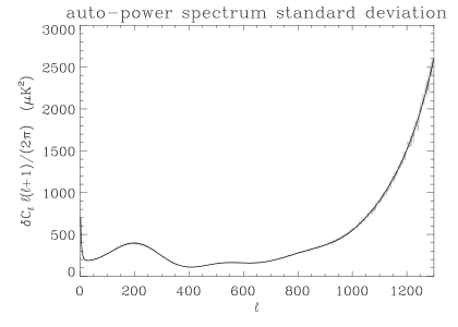
Figure 2: Standard deviation of the auto-power spectrum estimator. In grey we show the results obtained from 1000 Monte Carlo simulations, while the black line is obtained from equation 17.

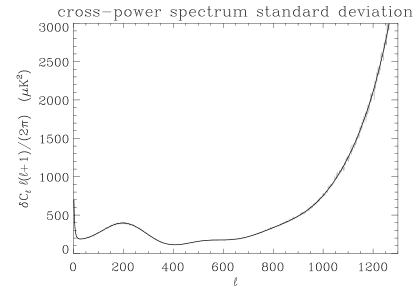
Figure 3: Standard deviation of the cross-power spectrum estimator. In grey we show the results obtained from 1000 Monte Carlo simulations, while the black line is obtained from equation 10.

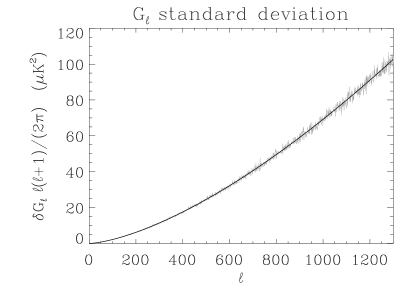
Figure 4: Standard deviation of the difference between the auto- and the cross-power spectrum estimator. In grey we show the results obtained from 1000 Monte Carlo simulations, while the black line is obtained from equation 24.

We now focus more directly on the efficiency of the Hausman test in identifying a residual bias in the auto-power spectrum. In order to achieve this goal, we simulate 300 further maps with a noise power spectrum ${C}_{\ell}^{N}$, and we compute the auto-power spectrum using a modified version of equation 7:

$$\widehat{C}_{\ell}=\frac{1}{2\ell+1}\sum_{m=-\ell}^{\ell}d_{\ell m}\overline{d_{\ell m}}-f_{n}C_{\ell}^{N}\mbox{ .}$$ (37)

In this way we simulate a wrong estimation of the noise power spectrum.

Then, for a fixed $f_{n}$, we compute $H_{\ell}$ and $B_{L}(r)$ for each simulation. We consider the three test statistics $s_{1}=\sup_{r}B_{L}(r)$, $s_{2}=\sup_{r}|B_{L}(r)|$ and $s_{3}=\int_{0}^{1}B_{L}^{2}(r)dr$, and the threshold values for the $68\%,95\%$ and $99\%$ probability. We used a thousand independent simulations with the value $f_{n}=1,$, corresponding to the case where our a priori knowledge of noise is correct, to tabulate the empirical distributions under this null hypothesis; results are reported in table 1.

Table 1: Threshold values under the null hypothesis

• 	$s_{1}$	$s_{2}$	$s_{3}$
  $68\%$	0.919	1.533	0.596
  $95\%$	1.818	2.550	1.926
  $99\%$	2.401	3.308	3.842

We then go on to compute $s_{1},s_{2}$ and $s_{3}$ under the alternatives $f_{n}\neq 1;$ the percentages of rejections provide an estimate of the power of these procedures in detecting a bias. Results are reported in tables 2-4, and are clearly very encouraging: the $s_{2}$ and $s_{3}$ test statistics enjoy $100\%$ power even in the presence of a mere $1\%$ misspecification of the noise angular power spectrum. Note that, as expected, $s_{1}$ is a unidirectional test, that is, it has no power in the case where noise is overestimated ($f_{n}>1)$; however, for such circumstances it would suffice to consider $s_{1}^{\prime}=\inf_{r}B_{L}(r)$ to obtain satisfactory power properties. In general, $s_{2}$ and $s_{3}$ should clearly be preferred for their robustness against a wider class of departures from the null.

Table 2: The power of the test $s_{1}$

• $f_{n}$	0.99	0.995	0.998	0.999	1.001	1.002	1.005	1.01
  $68\%$	1.00	1.00	0.79	0.54	0.15	0.08	0.01	0.00
  $95\%$	1.00	0.99	0.39	0.14	0.01	0.00	0.00	0.00
  $99\%$	1.00	0.96	0.16	0.05	0.00	0.00	0.00	0.00

Table 3: The power of the test $s_{2}$

• $f_{n}$	0.99	0.995	0.998	0.999	1.001	1.002	1.005	1.01
  $68\%$	1.00	1.00	0.54	0.27	0.53	0.82	1.00	1.00
  $95\%$	1.00	0.95	0.12	0.04	0.11	0.43	0.98	1.00
  $99\%$	1.00	0.76	0.04	0.00	0.03	0.12	0.95	1.00

Table 4: The power of the test $s_{3}$

• $f_{n}$	0.99	0.995	0.998	0.999	1.001	1.002	1.005	1.01
  $68\%$	1.00	0.99	0.57	0.33	0.45	0.74	1.00	1.00
  $95\%$	1.00	0.86	0.15	0.06	0.11	0.30	0.95	1.00
  $99\%$	1.00	0.58	0.03	0.01	0.02	0.08	0.76	1.00

5.1 Effect of partial sky coverage

In order to study the effect of partial sky coverage on the Hausman test, we repeated the Monte Carlo analysis considering the patch observed by BOOMERanG, covering $\sim 2\%$ of the full sky [38, 9]. We expect this to be a good limiting case, where any failures of the test due to partial sky coverage should clearly show up.

The main effect of partial sky coverage is, as well known, to produce correlations among spherical harmonic coefficients, that can be interpreted as a reduction of the effective number of degrees of freedom in the power spectrum [28].

Results are reported in tables 5-7. We stress that the power of the Hausman test, although reduced (as expected), is still very satisfactory. For instance, a misspecification of the noise level of the order of $5\%$ is detected $100\%$ of the times by $s_{2}$ and $99\%$ by $s_{3}$.

Table 5: The power of the test $s_{1}$ in the presence of partial sky coverage.

• $f_{n}$	0.95	0.96	0.97	0.98	0.99	1.01	1.02	1.03	1.04	1.05
  $68\%$	1.00	1.00	0.99	0.94	0.70	0.09	0.03	0.01	0.00	0.00
  $95\%$	1.00	1.00	0.97	0.75	0.35	0.01	0.00	0.00	0.00	0.00
  $99\%$	1.00	0.99	0.91	0.63	0.17	0.01	0.00	0.00	0.00	0.00

Table 6: The power of the test $s_{2}$ in the presence of partial sky coverage.

• $f_{n}$	0.95	0.96	0.97	0.98	0.99	1.01	1.02	1.03	1.04	1.05
  $68\%$	1.00	1.00	0.99	0.88	0.58	0.42	0.82	0.98	1.00	1.00
  $95\%$	1.00	1.00	0.95	0.67	0.26	0.18	0.54	0.91	0.99	1.00
  $99\%$	1.00	0.99	0.85	0.50	0.11	0.08	0.34	0.78	0.97	1.00

Table 7: The power of the test $s_{3}$ in the presence of partial sky coverage.

• $f_{n}$	0.95	0.96	0.97	0.98	0.99	1.01	1.02	1.03	1.04	1.05
  $68\%$	1.00	1.00	0.96	0.80	0.51	0.37	0.70	0.94	0.99	1.00
  $95\%$	1.00	0.96	0.82	0.53	0.16	0.13	0.35	0.73	0.95	0.99
  $99\%$	0.99	0.92	0.70	0.33	0.09	0.05	0.23	0.55	0.88	0.99

5.2 Polarization and 1/f noise correlated among different detectors

We move forward, analysing a more realistic case including polarization measurements in the presence of 1/f noise correlated among different detectors. This is achieved generating time ordered data with a scanning strategy and detectors noise properties similar to those of BOOMERanG-B03, where correlations of the order of $10\%$ are present (see table 7 in [9]), and the 1/f noise knee frequency is $\sim 0.07Hz$ (see figure 21 in [9]). The sky maps are then obtained using the ROMA IGLS polarization map-making code [39].

Polarization measurements provide six power spectra that can be used separately or combined to obtain a more efficient detection of the noise bias. The optimal combination of polarization power spectra is under investigation and will be addressed in a future paper. Here, in order to illustrate the method, we simply average the $B_{L}(r)$ obtained from each power spectrum.

Results are reported in tables 8-10. Once more the power of the Hausman test is reduced with respect to the full sky uncorrelated noise case, but is still satisfactory. For instance, a misspecification of the noise level of the order of $15\%$ is detected $\sim 100\%$ of the times with $95\%$ significance.

Table 8: The power of the test $s_{1}$ for polarization measurements with 1/f noise correlated among different detectors.

• $f_{n}$	0.80	0.85	0.90	0.95	0.98	1.02	1.05	1.10	1.15	1.20
  $68\%$	1.00	1.00	1.00	0.93	0.79	0.48	0.29	0.12	0.05	0.00
  $95\%$	1.00	1.00	0.89	0.47	0.21	0.06	0.04	0.02	0.01	0.00
  $99\%$	0.99	0.88	0.45	0.11	0.05	0.02	0.01	0.00	0.00	0.00

Table 9: The power of the test $s_{2}$ for polarization measurements with 1/f noise correlated among different detectors.

• $f_{n}$	0.80	0.85	0.90	0.95	0.98	1.02	1.05	1.10	1.15	1.20
  $68\%$	1.00	1.00	0.99	0.83	0.65	0.76	0.90	1.00	1.00	1.00
  $95\%$	1.00	0.99	0.73	0.29	0.12	0.17	0.39	0.86	0.99	1.00
  $99\%$	0.99	0.83	0.38	0.07	0.04	0.04	0.07	0.51	0.93	1.00

Table 10: The power of the test $s_{3}$ for polarization measurements with 1/f noise correlated among different detectors.

• $f_{n}$	0.80	0.85	0.90	0.95	0.98	1.02	1.05	1.10	1.15	1.20
  $68\%$	1.00	1.00	0.98	0.84	0.72	0.75	0.89	1.00	1.00	1.00
  $95\%$	1.00	0.95	0.61	0.21	0.14	0.17	0.36	0.76	0.96	1.00
  $99\%$	0.97	0.70	0.25	0.09	0.04	0.05	0.07	0.36	0.82	0.99

The Planck experiment will provide full sky polarization maps with pixel sensitivity similar to that of BOOMERanG-B03. Such a wide sky coverage will allow us to reach unprecedented accuracy in the estimated power spectra. The application of the Hausman test to Planck simulated maps will be the subject of a forthcoming paper.

6 Conclusions

We have discussed the analytic properties of the cross-power spectrum as an estimator of the angular power spectrum of the CMB anisotropies. The method is computationally convenient for very large data sets as those provided by WMAP or Planck and it provides unbiased estimates under very broad assumptions (basically, that noise is uncorrelated along different channels). It thus provides a robust alternative, where noise estimation and subtraction are not required. We also propose a new procedure for testing for the presence of residual bias due to inappropriate noise subtraction in pseudo-$C_{\ell}$ estimates (the Hausman test). The test compares the auto- and cross-power spectrum estimators under the null hypothesis. In the case of failure, the more robust cross-power spectrum should be preferred, while in the case of success both estimators could be used, and the choice should result from a trade-off between efficiency and robustness. We derive the analytic behaviour of this procedure under the null hypothesis, and use Monte Carlo simulations to investigate its power properties, which appear extremely promising. We leave for future research some further improvements of this approach, in particular, the use of bootstrap/resampling methods to make even the determination of confidence intervals independent from noise estimation. Finally, the optimal combination of polarization power spectra and the application of the Hausman test to the Planck satellite are currently under investigation.

Appendix

We recall the definition of the cross spectrum estimator (equation 11):

$$\widetilde{C}_{\ell}^{ij}=\frac{1}{2\ell+1}\sum_{m=-\ell}^{\ell}d_{\ell m}^{i}\overline{d_{\ell m}^{j}}=\frac{1}{2\ell+1}\sum_{m=-\ell}^{\ell}\left\{(a_{\ell m}+a_{\ell m}^{N_{i}})(\overline{a}_{\ell m}+\overline{a}_{\ell m}^{N_{j}})\right\}$$

$$=\frac{1}{2\ell+1}\sum_{m=1}^{\ell}\left\{(2|a_{\ell m}|^{2}+a_{\ell m}^{N_{i}}\overline{a}_{\ell m}+\overline{a}_{\ell m}^{N_{i}}a_{\ell m}+a_{\ell m}\overline{a}_{\ell m}^{N_{j}}+\overline{a}_{\ell m}a_{\ell m}^{N_{j}}+a_{\ell m}^{N_{i}}\overline{a}_{\ell m}^{N_{j}}+\overline{a}_{\ell m}^{N_{i}}a_{\ell m}^{N_{j}})\right\}$$

$$+\frac{1}{2\ell+1}\left\{(|a_{\ell 0}|^{2}+a_{\ell 0}^{N_{i}}a_{\ell 0}+a_{\ell 0}a_{\ell 0}^{N_{j}}+a_{\ell m}^{N_{i}}a_{\ell m}^{N_{j}})\right\}\mbox{ .}$$ (38)

It is easy to see that all summands in equation 38 are uncorrelated (albeit not independent), with variances given by

$$Var\left\{2|a_{\ell m}|^{2}\right\}=4C_{\ell},m=1,...,\ell,Var\left\{|a_{\ell 0}|^{2}\right\}=2C_{\ell}$$ (39)

$$Var\left\{a_{\ell m}^{N_{i}}\overline{a}_{\ell m}\right\}=Var\left\{\overline{a}_{\ell m}^{N_{i}}a_{\ell m}\right\}=C_{\ell}^{N_{i}}C_{\ell},m=0,...,\ell$$ (40)

$$Var\left\{a_{\ell m}^{N_{i}}\overline{a}_{\ell m}^{N_{j}}\right\}=Var\left\{\overline{a}_{\ell m}^{N_{i}}a_{\ell m}^{N_{j}}\right\}=C_{\ell}^{N_{i}}C_{\ell}^{N_{j}},m=0,...,\ell$$ (41)

whence we obtain

$$Var\left\{\widetilde{C}_{\ell}^{ij}\right\}=\frac{2}{(2\ell+1)^{2}}\sum_{m=1}^{\ell}\left\{2C_{\ell}+C_{\ell}^{N_{i}}C_{\ell}+C_{\ell}^{N_{j}}C_{\ell}+C_{\ell}^{N_{i}}C_{\ell}^{N_{j}}\right\}$$

$$+\frac{1}{(2\ell+1)^{2}}\left\{2C_{\ell}+C_{\ell}^{N_{i}}C_{\ell}+C_{\ell}^{N_{j}}C_{\ell}+C_{\ell}^{N_{i}}C_{\ell}^{N_{j}}\right\}$$

$$\hbox to0.0pt{\hss${}={}$}\frac{1}{2\ell+1}\left\{2C_{\ell}+C_{\ell}^{N_{i}}C_{\ell}+C_{\ell}^{N_{j}}C_{\ell}+C_{\ell}^{N_{i}}C_{\ell}^{N_{j}}\right\}\mbox{ .}$$ (42)

We show now that, for a single couple $(i,j),$ we have

$$Cov\left\{\widehat{C}_{\ell},\widetilde{C}_{\ell}^{ij}\right\}=\frac{2}{2\ell+1}\left\{C_{\ell}^{2}+\frac{C_{\ell}}{k}\left(C_{\ell}^{N_{i}}+C_{\ell}^{N_{j}}\right)+\frac{1}{k^{2}}C_{\ell}^{N_{i}}C_{\ell}^{N_{j}}\right\}\mbox{ .}$$ (43)

Indeed,

$$Cov\left\{\widehat{C}_{\ell},\widetilde{C}_{\ell}^{ij}\right\}=$$

$$=Cov\left[\left\{|a_{\ell m}|^{2}+a_{\ell m}\overline{a}_{\ell m}^{N}+\overline{a}_{\ell m}a_{\ell m}^{N}+|a_{\ell m}^{N}|^{2}\right\},\left\{|a_{\ell m}|^{2}+a_{\ell m}\overline{a}_{\ell m}^{N_{j}}+a_{\ell m}^{N_{i}}\overline{a}_{\ell m}+a_{\ell m}^{N_{i}}\overline{a}_{\ell m}^{N_{j}}\right\}\right]$$

$$=\frac{1}{(2\ell+1)^{2}}Cov\left[\left\{a_{\ell 0}^{2}+2a_{\ell 0}a_{\ell 0}^{N}+(a_{\ell 0}^{N})^{2}\right\},\left\{a_{\ell 0}^{2}+a_{\ell 0}a_{\ell 0}^{N_{j}}+a_{\ell 0}^{N_{i}}a_{\ell 0}+a_{\ell 0}^{N_{i}}a_{\ell 0}^{N_{j}}\right\}\right]$$

$$+\frac{1}{(2\ell+1)^{2}}\sum_{m=1}^{\ell}Cov\left[2\left\{|a_{\ell m}|^{2}+a_{\ell m}\overline{a}_{\ell m}^{N}+\overline{a}_{\ell m}a_{\ell m}^{N}+|a_{\ell m}^{N}|^{2}\right\},\right.$$ (44)

$$\left.\left\{2|a_{\ell m}|^{2}+a_{\ell m}\overline{a}_{\ell m}^{N_{j}}+\overline{a}_{\ell m}a_{\ell m}^{N_{J}}+a_{\ell m}\overline{a}_{\ell m}^{N_{i}}+\overline{a}_{\ell m}a_{\ell m}^{N_{i}}+a_{\ell m}^{N_{I}}\overline{a}_{\ell m}^{N_{j}}+\overline{a}_{\ell m}^{N_{I}}a_{\ell m}^{N_{j}}\right\}\right]$$

where

$$a_{\ell m}^{N}=\frac{1}{k}\sum_{i=1}^{k}a_{\ell m}^{N_{i}}\mbox{ .}$$ (45)

Now,

$$Cov\left[\left\{a_{\ell 0}^{2}+2a_{\ell 0}a_{\ell 0}^{N}+(a_{\ell 0}^{N})^{2}\right\},\left\{a_{\ell 0}^{2}+a_{\ell 0}a_{\ell 0}^{N_{j}}+a_{\ell 0}^{N_{i}}a_{\ell 0}+a_{\ell 0}^{N_{i}}a_{\ell 0}^{N_{j}}\right\}\right]$$ (46)

$$\hbox to0.0pt{\hss${}={}$}2\left\{C_{\ell}^{2}+\frac{C_{\ell}}{k}(C_{\ell}^{N_{i}}+C_{\ell}^{N_{j}})+\frac{1}{k^{2}}C_{\ell}^{N_{i}}C_{\ell}^{N_{j}}\right\}$$

and likewise

$$Cov\left[2\left\{|a_{\ell m}|^{2}+a_{\ell m}\overline{a}_{\ell m}^{N}+\overline{a}_{\ell m}a_{\ell m}^{N}+|a_{\ell m}^{N}|^{2}\right\},\right.$$

$$\left.\left\{2|a_{\ell m}|^{2}+a_{\ell m}\overline{a}_{\ell m}^{N_{j}}+\overline{a}_{\ell m}a_{\ell m}^{N_{J}}+a_{\ell m}\overline{a}_{\ell m}^{N_{i}}+\overline{a}_{\ell m}a_{\ell m}^{N_{i}}+a_{\ell m}^{N_{I}}\overline{a}_{\ell m}^{N_{j}}+\overline{a}_{\ell m}^{N_{I}}a_{\ell m}^{N_{j}}\right\}\right]$$

$$\hbox to0.0pt{\hss${}={}$}4\left\{C_{\ell}^{2}+\frac{C_{\ell}}{k}(C_{\ell}^{N_{i}}+C_{\ell}^{N_{j}})+\frac{1}{k^{2}}C_{\ell}^{N_{i}}C_{\ell}^{N_{j}}\right\}\mbox{ .}$$ (47)

Hence,

$$Cov\left\{\widehat{C}_{\ell},\widetilde{C}_{\ell}^{ij}\right\}=\frac{2}{(2\ell+1)^{2}}\left\{C_{\ell}^{2}+\frac{C_{\ell}}{k}(C_{\ell}^{N_{i}}+C_{\ell}^{N_{j}})+\frac{1}{k^{2}}C_{\ell}^{N_{i}}C_{\ell}^{N_{j}}\right\}$$

$$+\frac{4}{(2\ell+1)^{2}}\sum_{m=1}^{\ell}\left\{C_{\ell}^{2}+\frac{C_{\ell}}{k}(C_{\ell}^{N_{i}}+C_{\ell}^{N_{j}})+\frac{1}{k^{2}}C_{\ell}^{N_{i}}C_{\ell}^{N_{j}}\right\}$$

$$\hbox to0.0pt{\hss${}={}$}\frac{2}{2\ell+1}\left\{C_{\ell}^{2}+\frac{C_{\ell}}{k}(C_{\ell}^{N_{i}}+C_{\ell}^{N_{j}})+\frac{1}{k^{2}}C_{\ell}^{N_{i}}C_{\ell}^{N_{j}}\right\}$$ (48)

as claimed.

References

References

- [1] Smoot G F et al1992 ApJ 396 L1
- [2] Hanany S et al2000 ApJ 545 L5
- [3] de Bernardis Pcet al2000 Nature 404 955
- [4] Miller A D et al1999 ApJ 524 L1
- [5] Halverson N W et al2002 ApJ 568 38
- [6] Netterfield C B et al2002 ApJ 571 604
- [7] de Bernardis P et al2002 ApJ 564 559
- [8] Ruhl J et al2003 ApJ 599 786
- [9] Masi S et al2005 Preprint astro-ph/0507509
- [10] Jones W C et al2005 Preprint astro-ph/0507494
- [11] Piacentini F et al2005 Preprint astro-ph/0507507
- [12] Montroy T E et al2005 Preprint astro-ph/0507514
- [13] MacTavish C J et al2005 Preprint astro-ph/0507503
- [14] Grainge K et al2003 MNRAS 341 L23
- [15] Benoit A et al2003 A&A 399 L19
- [16] Pearson T J et al2003 ApJ 591 556
- [17] Kuo C L et al2004 ApJ 600 32
- [18] O’Dwyer I J et al2005 ApJS 158 93
- [19] Bennett C L et al2003 ApJS 148 1
- [20] Bond J R , Jaffe A H and Knox L E 1998 Phys. Rev. D 57 2117
- [21] Borrill J 1999 AIP Conf Proc 476 277B
- [22] Efstathiou G 2003 Preprint astro-ph/0307515
- [23] Oh S P , Spergel D and Hinshaw G 1999 ApJ 510 550
- [24] Wandelt B, Hivon E and Gorski K M 2001 Phys. Rev. D 64h3003W
- [25] Wandelt B and Hansen F K 2003 Phys. Rev. D 67b3001W
- [26] Challinor A et al2003 NewAR 47 995C
- [27] Szapudi I et al2001 ApJ 561 L11S
- [28] Hivon E et al2002 ApJ 567 211
- [29] Balbi A et al2002 A&A 395 417b
- [30] Hansen F K, Gorski K M and Hivon E 2002 MNRAS 336 1304h
- [31] Delabrouille J, Cardoso J F and Patanchon G 2003 MNRAS 346 1089
- [32] Hinshaw G et al2003 ApJS 148 135
- [33] Polenta G et al2002 ApJ 572 L27
- [34] Komatsu E et al2003 ApJS 148 119
- [35] Santos M G 2003 MNRAS 341 623
- [36] Billingsley P 1968 Convergence of Probability Measures (J.Wiley)
- [37] Borodin A and Salminen P 1996 Handbook of Brownian Motion: Facts and Formulae (Birkhauser)
- [38] Montroy T E et al2003 NewAR 47 1057
- [39] De Gasperis G et al2005 A&A 436 1159