CMB-Cluster Lensing

Abstract

Clusters of galaxies are powerful cosmological probes, particularly if their masses can be determined. One possibility for mass determination is to study the cosmic microwave background (CMB) on small angular scales and observe deviations from a pure gradient due to lensing of massive clusters. I show that, neglecting contamination, this technique has the power to determine cluster masses very accurately, in agreement with estimates by Seljak and Zaldarriaga (1999). However, the intrinsic small scale structure of the CMB significantly degrades this power. The resulting mass constraints are useless unless one imposes a prior on the concentration parameter $c$. With even a modest prior on $c$, an ambitious CMB experiment ($0.5^{\prime}$ resolution and $1\mu K$ per pixel) could determine masses of high redshift ($z>0.5$) clusters with $\sim 30\%$ accuracy.

I Introduction

Clusters of galaxies are powerful cosmological probes. The abundance of clusters is very sensitive to the amplitude of fluctuations in the mass density field. For example, the present-day mass distribution of clusters offers perhaps the cleanest way to measure the normalization of the matter power spectrum Eke et al. (1996); Henry (1997); Viana and Liddle (1999); Reiprich and Böhringer (2002); Ikebe et al. (2002); Schuecker et al. (2003a); Pierpaoli et al. (2003); Allen et al. (2003); Viana et al. (2003); Dodelson (2003a); Rozo et al. (2004). As we gain the ability to probe the cluster abundance at high redshifts, we can hope to measure the evolution of this normalization, an evolution which is sensitive to the dark energy and its equation of state Haiman et al. (2001); Wang and Steinhardt (1998); Schuecker et al. (2003b).

Because the mass function varies so rapidly with mass, accurate mass determination is critical if cluster constraints are to realize their potential. Finding clusters is not enough: even if a method finds all clusters and returns no false positives, it still does not necessarily have constraining power. It is quite possible that one technique will be optimal for finding clusters while another is a more powerful probe of cluster masses. For example, radio surveys which can measure the Sunyaev-Zel’dovich effect are very promising ways of detecting clusters even at high redshift White (2003). But they do not necessarily yield an accurate mass estimator. In contrast, weak gravitational lensing has drawbacks as a cluster finder Metzler et al. (2001); White et al. (2002) but is potentially a powerful way of measuring mass Kaiser and Squires (1993); Squires and Kaiser (1996); Hoekstra (2001, 2003); Schneider (2003); Dodelson (2003b).

While lensing of background galaxies has been studied in depth over the last decade, lensing of the cosmic microwave background (CMB) has not been explored as carefully, mainly because the angular resolution needed to see the predicted signal is only now being attained or planned Kosowsky (2003); Wootten (2002); Stark et al. (1998). Here I discuss how accurately cluster masses can be determined with observations of small angle ($\sim 1^{\prime}$) observations of the CMB.

On these very small scales, to a first approximation the background primordial CMB is a gradient. The photons passing close to the center of the cluster get deflected so that they appear to be originating further away from the cluster center. On the cool side of the gradient, this means the temperature is slightly hotter than it would appear without lensing, and on the hot side slightly cooler. So, subtracting off the dipole, the lensing pattern is quite distinctive Seljak and Zaldarriaga (1999); Zaldarriaga (2000), as shown in Fig. 1.

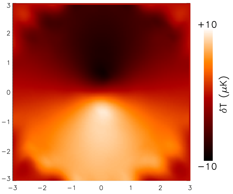
Figure 1: Idealized temperature pattern due to lensing of a cluster. Here, the background CMB is assumed to be a pure gradient with strength $T_{y}=13\mu$K arcmin^-1 and this gradient has been removed. The cluster, at redshift 1 with a mass $m_{200}=10^{15}h^{-1}M_{\odot}$, has an NFW profile. The area shown is within the virial radius of $3.3^{\prime}$. Jaggedness at the edge of the map is an indication of finite size $(0.5^{\prime})$ of the (noiseless) pixels.

Although there are many possible contaminants to this signal, its distinctive morphology allows one to hope that the signal can be extracted from any sources of noise Seljak and Zaldarriaga (1999); Holder and Kosowsky (2004); Vale et al. (2004). Here I examine how accurately CMB lensing can determine the masses of clusters, accounting for the small scale structure present in the CMB, i.e., the fact that the background CMB is not a pure gradient. There are two sources of this small scale structure: one is the power which remains in the damping tail of the primordial ($z\sim 1100$) spectrum and the other is lensing by structures along the line of sight. Figure 2 gives an indication of the strength of the signal and the contributions from the CMB, which I will call CMB noise. The CMB noise dwarfs the signal on “large” scales. We will see that this significantly impairs the constraining power of CMB-cluster lensing.

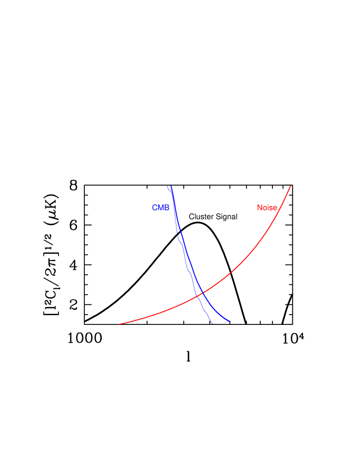
Figure 2: Anticipated signal from the lensing of a massive cluster and noise in $l$-space. The cluster has mass $10^{15}h^{-1}M_{\odot}$ and is at redshift $1$. The light CMB curve is without lensing along the line of sight; the heavy CMB line includes this effect. The instrumental noise corresponds to a $0.5^{\prime}$ resolution experiment with $1\mu$K noise per pixel.

Section II describes the model for the mass density I will use throughout and the ensuing constraints if CMB noise were absent. Section III shows how CMB noise pollutes the signal and which modes retain their power. Figures 8-10 summarize the main results of the paper and can be understood without reading the text. Finally, in the conclusion, I emphasize some of the simplifications made throughout.

II Constraints Neglecting CMB Noise

Numerical simulations Navarro et al. (1997, 1996) find that clusters obey a Navarro-Frenk-White (NFW) profile,

$$\rho(r)={A\over r(cr+r_{v})^{2}}$$ (1)

with two parameters the virial radius $r_{v}$ and concentration $c$. The virial radius is the radius within which the enclosed mass, $m_{200}$, is $200$ times the average mass in a critical density universe in the same volume. Therefore, it is convenient to use $m_{200}$ instead of the virial radius as the second parameter,

$$m_{200}={800\pi\over 3}\rho_{\rm cr}(z)r_{v}^{3}$$ (2)

where the evolving critical density $\rho_{\rm cr}(z)$ is expressed in terms of the Hubble rate, $3H^{2}(z)/8\pi G$. The amplitude of the density is then

$$A={m_{200}c^{2}\over 4[\ln(1+c)-c/(1+c)]}.$$ (3)

Throughout I will take $c=5$ since this is a typical value emerging from simulations Bullock et al. (2001a), although it does not reflect the changes of $c$ with redshift or the (slight) changes with mass.

Given this mass distribution, we can ask how the observed signal $\tilde{T}$ in the CMB is affected by the lens. Lensing can be included by Taylor expanding the temperature field around the unlensed field $T$:

$$\tilde{T}(\vec{\theta}) = T(\vec{\theta}-\vec{\delta\theta})\simeq T(\vec{\theta})-\vec{\delta\theta}\cdot{\partial T\over\partial\vec{\theta}}$$ (4)

$$= -\vec{\delta\theta}_{\rm cl}\cdot{\partial T\over\partial\vec{\theta}}+\left(T(\vec{\theta})-\vec{\delta\theta}_{\rm lss}\cdot{\partial T\over\partial\vec{\theta}}\right)$$

where $\vec{\delta\theta}$ is the deflection angle due to lensing along the line of sight due to the cluster (_cl subscript) and unassociated large scale structure (_lss subscript). Seljak and Zaldarriaga Seljak and Zaldarriaga (1999); Zaldarriaga (2000) realized that on small scales the primoridial CMB has little structure so $\partial T/\partial\vec{\theta}$ in the first term can be set to a constant. Aligning the $y$-axis with this vector and calling the constant $T_{y}$ leads to

$$\tilde{T}(\vec{\theta})\simeq-{\delta\theta}_{\rm cl,y}(\vec{\theta})T_{y}+\left(T(\vec{\theta})-\vec{\delta\theta}_{\rm lss}\cdot{\partial T\over\partial\vec{\theta}}\right).$$ (5)

To be clear, $\delta\theta_{\rm cl,y}(\vec{\theta})$ is the $y$-component of the deflection angle due to the cluster at angular position $\vec{\theta}$, and $T_{y}$ is the primordial gradient at the center of the cluster, the derivative of the temperature field with respect to $\theta_{y}$. The term in parentheses in Eq. (5) is the lensed CMB temperature with mean zero and variance determined by the set of $C_{l}$’s appropriate for the chosen cosmology. Note from Fig. 2 that lensing due to large scale structure gives additional power to the CMB at the scales of interest.

The deflection angle due to the NFW profile is known to be Wright and Brainerd (2000); Dodelson and Starkman (2003)

$$\vec{\delta}\theta_{\rm cl}(\vec{\theta})=-{16\pi GA\over cr_{v}}{\vec{\theta}\over\theta}{d_{SL}\over d_{S}}g(d_{L}\theta c/r_{v})$$ (6)

where the distances are angular diameter distances (e.g. the angular diameter distance between the source and the lens $d_{SL}$ is $(\chi_{S}-\chi_{L})/(1+z_{s})$ in a flat universe where $\chi$ is the comoving distance out to the relevant redshift). The function $g$ is of order unity and peaks when its argument is equal to $1.3$:

$$g(x)={1\over x}\cases{\ln(x/2)+{\ln(x/[1-\sqrt{1-x^{2}}]\over\sqrt{1-x^{2}}})&$x<1$\cr\ln(x/2)+{\pi/2-{\rm arcsin}(1/x)\over\sqrt{x^{2}-1}}&$x>1$\cr}.$$ (7)

Figure 1 shows the temperature pattern on the sky – with the background gradient removed – due to lensing of an NFW cluster with mass $10^{15}h^{-1}M_{\odot}$ at redshift 1. Note the distinctive double lobe pattern on either side of the cluster. Here I have set the background gradient $(T_{y})$ to $\sigma_{\rm grad}=13\mu$K/arcmin, its rms value in a flat cosmology with $\Omega_{\Lambda}=0.7,\Omega_{b}=0.04,h=0.7,\sigma_{8}=0.9,\tau=0.1$, and primordial spectral index $n=1$. The hot and cold spots on either side of the cluster are then $9\mu$K an arcmin away from the cluster center, dropping off to $7\mu$K at the virial radius of $3.3^{\prime}$.

Figure 3: Contributions to the mass constraint as a function of distance from the cluster center. Although the largest individual contribution comes from pixels much closer to the center than the virial radius as indicated by the solid curve, the pixels at the edge contribute the most in total because there are more of them. This is in the unrealistic case where only uniform instrumental noise is considered.

The mild drop of the signal means that the outermost regions of the cluster contribute most to the mass constraints when only instrumental noise is considered. To see this and to contrast with the more realistic situation when other sources of noise are included later on, consider the Fisher matrix which determines the constraints on the parameters $m_{200}$ and $c$:

$$F_{\alpha\beta}=\sigma_{\rm grad}^{2}\sum_{i,j=1}^{N}{\partial\delta\theta_{\rm cl,y}(\theta_{i})\over\partial\lambda_{\alpha}}\left(C^{-1}\right)_{ij}{\partial\delta\theta_{\rm cl,y}(\theta_{j})\over\partial\lambda_{\beta}}.$$ (8)

Here $\alpha,\beta$ label the two parameters ($\lambda_{1}=\ln m_{200},\lambda_{2}=\ln(c)$), while $i,j$, which are summed over, label the $N$ pixels in the map. If the noise matrix is diagonal with uniform noise $\sigma_{n}$ in all pixels, which might be true if only instrumental noise is considered, then the fractional constraint on the mass for example reduces to a single sum over all pixels:

$$F_{11}={\sigma_{\rm grad}^{2}\over\sigma_{n}^{2}}\sum_{i=1}^{N}\left({\partial\delta\theta_{\rm cl,y}(\theta_{i})\over\partial\ln m_{200}}\right)^{2}\equiv\sum_{i=1}^{N}f_{11,i}.$$ (9)

That is, each pixel contributes an amount $f_{11,i}$ to the mass constraint. Figure 3 shows that although the largest contribution comes from the pixels a distance $0.4r_{v}$ from the cluster center, when we sum over all pixels in an annulus [$\propto\int drrf_{11}(r)$], the annulus with the largest radius has the most constraining power.

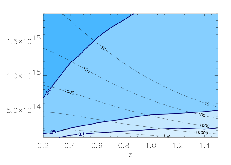
Figure 4: Shaded contours show $1$-$\sigma$ projections of $\delta M/M$ of a cluster from a CMB experiment with noise per pixel of 1$\mu$K and pixel size $0.5^{\prime}$. These constraints do not include CMB noise. Dashed lines indicate values for the cumulative number of clusters (total number above the given mass and redshift) expected in the standard $\Lambda$CDM cosmology ($\sigma_{8}=0.85$).

If this conclusion held up as more sources of noise were included, it would have dramatic implications for which clusters were best suited to be studied by CMB lensing. To see this, I will examine the constraints on the mass and concentration of a cluster by using all pixels out to the virial radius. Beyond the virial radius, the profile begins to deviate from an NFW profile. While we have no way of knowing in advance where the virial radius is, one can imagine fitting for all pixels within say $10^{\prime}$ and getting non-negligible signal only from distances smaller than the virial radius. As we will see in §III, this discussion is academic because CMB noise renders pixels near the virial radius much less useful.

With this strategy, we would constrain the mass of a cluster at lower redshift more tightly than one (of the same mass) at high redshift because the low redshift object subtends a larger fraction of the sky. We can see this in Figure 4 which shows the $1$-$\sigma$ constraints on $m_{200}$ from an idealized CMB experiment with $\sigma_{n}=1\mu$K and pixel size $\Delta=0.5^{\prime}$. The constraints in this unrealistic situation are astounding, percent level errors on the mass, even after marginalizing over the concentration. Note the trend that for fixed mass, the constraints do indeed get stronger as the cluster moves to lower redshift. The dashed lines in the figure show the cumulative number of clusters expected at each mass and redshift. For example, the point $z=0.2,m_{200}=5\times 10^{14}h^{-1}M_{\odot}$ is intersected (roughly) by the contour labeled “10000.” In this cosmology then, we expect $10^{4}$ clusters over the whole sky with mass greater than $5\times 10^{14}h^{-1}M_{\odot}$ at redshifts greater than $0.2$. (These contours were obtained using the Jenkins mass function Jenkins et al. (2001).)

III Constraints Including CMB Noise

To include noise from the CMB, I generate a set of $C_{l}$’s for the chosen cosmology including lensing due to large scale structure using CMBFAST Seljak and Zaldarriaga (1996). The new covariance matrix is then

$$C=C^{\rm noise}+\sum_{l}{2l+1\over 4\pi}C_{l}P_{l}(\cos\theta_{ij})$$ (10)

where $\theta_{ij}$ is the angular distance between pixels $i$ and $j$, and $C^{\rm noise}$ includes instrumental noise, assumed to be diagonal with variance $\sigma_{n}^{2}$.

In the presence of this new source of noise, it is useful again to ask which modes contribute most to the mass constraint. Now though, since the covariance matrix is not diagonal, we need to generalize Eq. (9). If we diagonalize the full covariance matrix

$$W=U^{t}C^{-1}U,$$ (11)

with the eigenvalues contained in the diagonal matrix $W$ then the Fisher matrix of Eq. (9) can still be written as a sum of weights, but now the sum is not over pixels but over modes. That is, the contribution of a given mode to the mass constraint is

$$f_{11,i}=W_{i}\sigma_{\rm grad}^{2}\left[\sum_{j}{\partial\delta\theta_{\rm cl,y}(\theta_{j})\over\partial\ln m_{200}}U_{ji}\right]^{2}.$$ (12)

The eigenvector associated with this mode is $\sum_{j}U_{ji}T(\theta_{j})$.

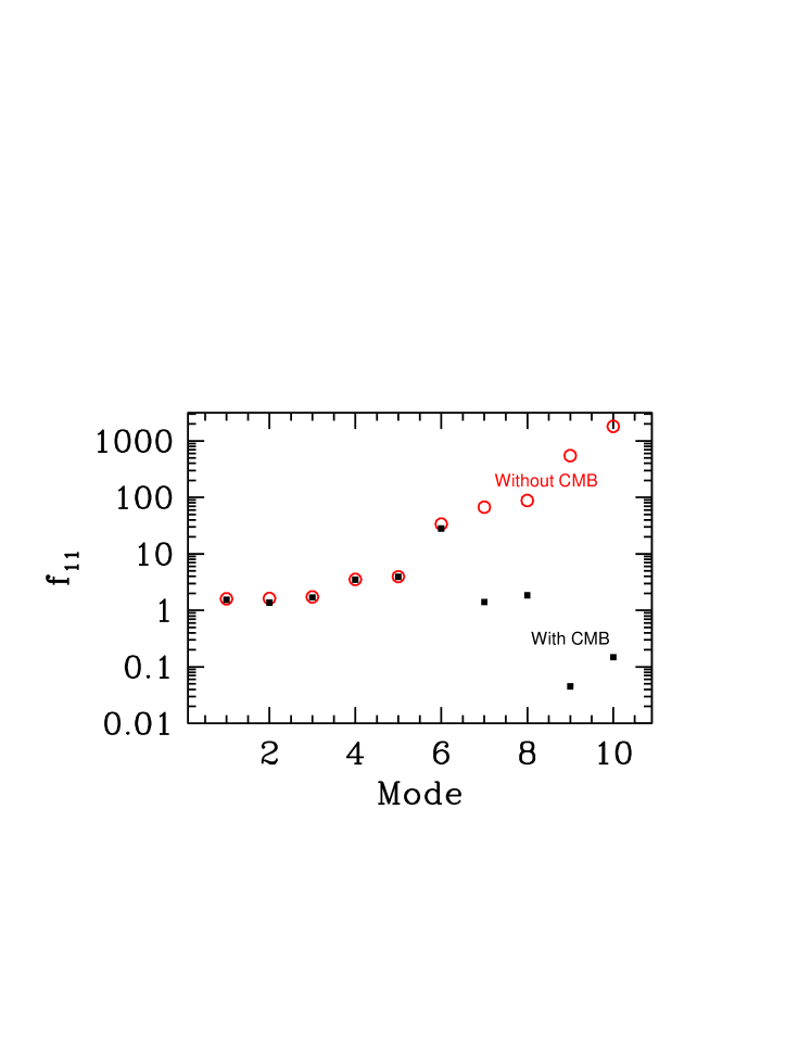
Figure 5: Constraining power of each of the top $10$ modes when CMB noise is not included (red open circles) and when it is (black solid squares). The modes are linear combinations of the pixels. While of order ten modes are useful in the absence of CMB noise, only one mode (mode 6 here) contributes significantly to the mass constraints when CMB noise is taken into account.

Fig. 5 illustrates how the signal in many modes is contaminated by CMB noise. Consider first the (red) circles which show $f_{11}$ for all the modes in the absence of CMB noise. The mode with the highest constraining power is depicted in the left panel of Fig. 6: it is essentially a gradient. Indeed, you can quickly estimate the mass constraint (with fixed concentration) from this mode: $f_{11}$ is of order $2000$, leading to $\delta m_{200}/m_{200}\sim 1/\sqrt{2000}\sim$ a few percent, in agreement with the result for a cluster with $m_{200}=10^{15}h^{-1}M_{\odot}$ at $z=1$ shown in Fig. 4. The filled squares in Fig. 5 portray a much different picture when CMB noise is accounted for. Now there is only one mode with $f_{11}>10$; it is shown in the right panel of Fig. 6. It is sensitive to the difference in the cluster signal in the outer and inner parts of the cluster. This mode cannot be reproduced by the CMB because the CMB lacks the necessary small scale power, but the signal in this mode is also quite a bit smaller. Recall from Fig. 1 that the signal changes only mildly from its peak to its value at the virial radius.

     

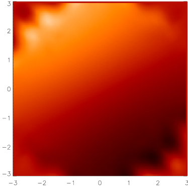
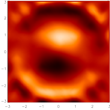
Figure 6: Left panel: The mode which is most constraining in the absence of CMB noise, but which gets annihilated when this noise is included. This is mode 10 in Fig. 5. Right panel: The one mode (mode 6 in Fig. 5) which contributes significantly to the constraints when CMB noise is included.

CMB-Cluster lensing then is sensitive not to the strength of the signal in both the hot and the cold spots, but rather to the structure of the signal in each. This changes the calculus of moving to lower redshift. All pixels on one side of the cluster no longer are weighted equally, so there is no longer an advantage in the larger clusters at low redshift.

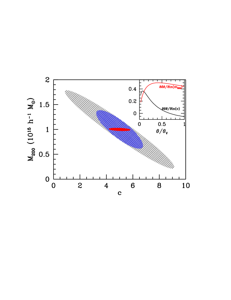
Figure 7: Constraints on the mass and concentration of a $10^{15}h^{-1}M_{\odot}$ cluster at redshift 1 with pixel size $0.5^{\prime}$ and noise $1\mu$K. Inner solid (red) ellipse does not account for CMB noise; largest (black) ellipse does; and medium-sized (blue) ellipse includes a $25\%$ prior on concentration $c$. Inset in upper right demonstrates why CMB noise induces degeneracy between $c$ and $m_{200}$. Shown are the derivatives of the deflection angle with respect to these two parameters. Note that the deflection angle – and hence the signal – is sensitive to the concentration only close to the cluster center.

Figure 7 shows how the constraints change on an individual cluster when CMB noise is taken into account. The innermost ellipse shows the constraint on a massive cluster before accounting for CMB noise. While the concentration is not pinned down with very high accuracy, the mass is. When CMB noise is introduced, there is a degeneracy between concentration and mass. The inset in Fig. 7 gives a hint as to the origin of this degeneracy. The concentration parameter affects the deflection angle, and hence the signal, only close to the cluster center. Increasing the mass, on the other hand, increases the signal everywhere within the virial radius. Without CMB noise, all pixels at distances $\theta\mathrel{\mathchoice{\lower 3.6pt\vbox{\halign{$\mathsurround=0pt\displaystyle\hfil#\hfil$\cr>\crcr\sim\crcr}}}{\lower 3.6pt\vbox{\halign{$\mathsurround=0pt\textstyle\hfil#\hfil$\cr>\crcr\sim\crcr}}}{\lower 3.6pt\vbox{\halign{$\mathsurround=0pt\scriptstyle\hfil#\hfil$\cr>\crcr\sim\crcr}}}{\lower 3.6pt\vbox{\halign{$\mathsurround=0pt\scriptscriptstyle\hfil#\hfil$\cr>\crcr\sim\crcr}}}}0.5\theta_{V}$ therefore contribute to help pin down $m_{200}$. The concentration is then determined by the innermost region, with its much smaller number of pixels; hence the concentration is known much less accurately. In the presence of CMB noise the situation changes: now the most important mode measures the difference between the signal in the inner and outer regions. Increasing the signal in the outer region by raising the mass can be offset by increasing the signal in the innermost region by raising the concentration. Therefore, only the sum of the two parameters is well constrained.

The mass-concentration degeneracy can be broken if we use the knowledge obtained from simulations Jing (2000); Bullock et al. (2001b) about the relation between the two. Imposing a prior on $c$ with a $25\%$ uncertainty leads to the intermediate ellipse in Fig. 7. The errors on the mass of this cluster then get reduced to useful levels. Even a more conservative prior on $c$ of $50\%$ leaves the mass errors quite tight: the factor of two increase in the $c$ prior leads to only a $\sim 40\%$ increase in the mass error.

Figure 8 shows the fractional uncertainty on cluster masses when all forms of noise considered above are included. The errors are above $50\%$ for clusters with mass below $10^{15}h^{-1}M_{\odot}$ even with the ambitious assumptions for noise and resolution. Note also that the uncertainties now get larger as the cluster moves to lower redshift. Although the cluster abundance depends heavily on $\sigma_{8}$, so the numbers in Fig. 8 (which assume $\sigma_{8}=0.85$) are only a guess, it is unlikely that there will be more than a handful of clusters for which CMB lensing will determine the mass to better than $50\%$. One possibility for a small scale CMB experiment is to sit on these handful (which are first identified in optical or Sunyaev-Zel’dovich surveys).

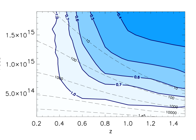
Figure 8: Fractional uncertainty on cluster mass from a CMB experiment with pixel size $0.5^{\prime}$ and noise $1\mu$K. Contours are as described in Fig. 4. The constraints here include CMB noise.

On the other hand, CMB-cluster lensing does enable us to determine a combination of the mass and concentration. One way to exploit this is to impose a prior on the concentration. Fig. 9 shows the resultant mass constraints with a $25\%$ prior on the concentration. With this prior, we can obtain masses accurate to $50\%$ for tens of thousands of clusters with masses above $2\times 10^{14}h^{-1}M_{\odot}$ at redshifts above $0.4$. The uncertainties go down to less than $30\%$ for the hundreds of clusters at redshifts greater than $\sim 0.8$ and masses above $\sim 5\times 10^{14}h^{-1}M_{\odot}$. These constraints could prove very useful in determining dark energy parameters. Alternatively, one could use the constraint on the mass/concentration in the context of a halo model Rozo et al. (2004).

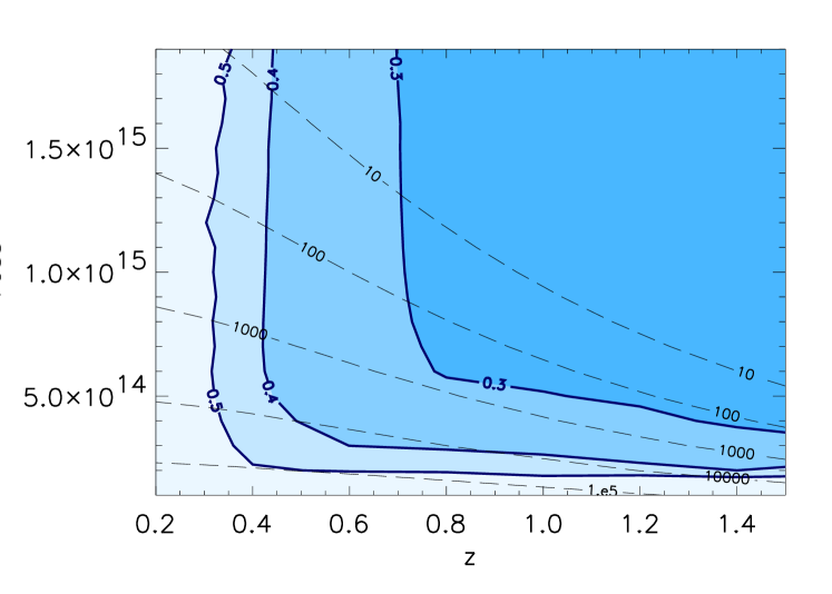
Figure 9: Same as Figure 8 except that here a $25\%$ prior is imposed on concentration $c$.

The above constraints were for an ambitious CMB experiment with noise per pixel of $1\mu$K and $0.5^{\prime}$ pixels. Figure 10 shows how well less ambitious experiments would do in determining the mass of a $10^{15}h^{-1}M_{\odot}$ cluster at $z=1$. Apparently pixel sizes must be smaller than $\sim 1.5^{\prime}$ and noise per pixel smaller than $5\mu$K for any reasonable constraints on cluster masses even including a concentration prior. This would seem to rule out CMB lensing in Planck as a useful tool for measuring cluster masses.

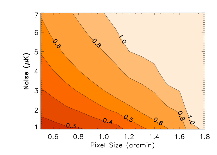
Figure 10: Constraints on the mass of a cluster at redshift 1 with $m_{200}=10^{15}h^{-1}$ Mpc including CMB noise and a prior on the concentration parameter. The point at bottom left here corresponds to the ($1,10^{15}$) point in Fig. 9.

IV Conclusion

Since gravitational lensing is directly sensitive to the mass of a cluster, it seduces us into hoping that we can reject more traditional phenomenological mass indicators such as X-ray temperature and galaxy counts. In the case considered here, lensing of the CMB, unavoidable realities spoil some of this allure. Since the primordial CMB does have some small scale structure, this CMB noise significantly degrades the constraining potential of the lensed field. The constraints may still prove useful in constraining cosmological parameters such as the dark energy equation of state, but we will have to include this degradation when evaluating different experimental proposals.

While I believe this work is an important step on the road to assessing the utility of CMB-cluster lensing, it is incomplete in several ways. First, I have neglected a number of other contaminants such as point sources, the thermal Sunyaev-Zel’dovich effect, and the kinetic Zel’dovich effect. It is at least conceivable that these other effects differ sufficiently in frequency dependence and spatial morphology from the cluster lensing signal that they will not further degrade the projected constraints much. For example, if the morphology of the kinetic Sunyaev-Zel’dovich effect is much different from that depicted in the right panel of Fig. 6, then it would have no impact on the mass determination, for we have seen that this is the mode which most tightly constraints the mass. Second, I have assumed a particularly simple parametrized form for the cluster mass distribution. Accounting for asphericity and substructure requires numerical simulations Holder and Kosowsky (2004); Vale et al. (2004), and these effects might add further noise to the mass estimators. Note that all of these effects would serve only to degrade the mass constraints further.

To close on a positive note, I point out that CMB experiments have consistently exceeded our expectations. There is thus every reason to believe that the high resolution, low noise experiments anticipated here will take place. If they do, then – along with input from numerical simulations such as the correlation between mass and concentration – we can hope to obtain interesting limits on the masses of thousands of clusters from CMB maps.

Note: After this work was completed (but before it was circulated), Holder and Kosowsky Holder and Kosowsky (2004) and Vale, Amblard, and White Vale et al. (2004) put out preprints studying very similar issues. Although we reached the same general conclusion – realistic effects degrade the ability of CMB-cluster lensing to determine masses – our papers are by and large complementary. While I have used analytic techniques and therefore simplified cluster models, the other two papers use more realistic numerical simulations. The simplicity has allowed me to provide quantitative measures of the efficiency of CMB-cluster lensing for a wide range of cluster masses, redshifts, noise levels, and pixel sizes. Ultimately, these estimates will need to be reinforced with the realistic simulations performed in Holder and Kosowsky (2004); Vale et al. (2004).