Accurate Modelling of Relativistic Iron Lines from Accretion Discs

Abstract

Observations of fluorescent iron lines from accreting black holes provide one of the best tests of strong field gravity available to date, and the only current observational tool to probe black hole spacetime. However, the two most widely used models for spectral fitting (diskline, laor) are over a decade old and have significant limitations. We present a new code for calculating these effects which will be incorporated within the XSPEC package.

1 Introduction

Material in an accretion disk around a black hole is orbiting at high velocity, close to the speed of light, in a strong gravitational potential. Hence its emission is distorted by doppler shifts, length contraction, time dilation, gravitational redshift and lightbending. The combined impact of these special and general relativistic effects was first calculated in the now seminal paper of Cunningham (1975),[1]  where he used a transfer function to describe the relativistic effects. Any sharp spectral features, such as the iron fluorescence line produced by X-ray illumination of an accretion disc is transformed into broad, skewed profile whose shape is given directly by the transfer function.[2]

Observationally, evidence for a relativistically smeared iron line first came from the ASCA observation of the active galactic nuclei (AGN) MCG-6-30-15.[3]  Further observations showed evidence for the line profile being so broad as to require a maximally spinning black hole.[4]  More recent data from XMM are interpreted as showing that the line is even wider than expected from an extreme Kerr disk, requiring direct extraction of the spin energy from the central black hole as well as the immense gravitational potential.[5]

While there are many caveats on extracting the line profile from the continuum,[7] the dramatic results from MCG-6-30-15 plainly also require that the extreme relativistic effects are well modelled. There are two models which are currently widely available to the observational community, within the XSPEC spectral fitting package, diskline [2] and laor. [6]  The analytic diskline code models the line profile from an accretion disc around a Schwarzschild black hole (so of course cannot be used to describe the effects in a Kerr geometry). Also, it does not include the effects of lightbending and hence does not accurately calculate all the relativistic effects for $r<20r_{g}$ (where $r_{g}=GM/c^{2}$). By contrast, the laor model numerically calculates the line profile including lightbending for an extreme Kerr black hole, but uses a rather small set of tabulated transfer functions which limit its resolution and accuracy (see Section 3).

While there are other relativistic codes in the literature which do not suffer from these limitations, these are not generally readily and/or easily available for observers to use. There is a clear need for a fast, accurate, high resolution code which can be used to fit data from the next generation of satellites. Here we give brief results from our new code for computing the relativistic iron line profile in both Schwarzschild and Kerr metrics. We compare this with the diskline and laor models in XSPEC, demonstrating the limitations and assumptions inherent in these previous codes.

2 Calculating Strong Gravitational Effects

A line of rest energy $E_{int}$ emitted with rest frame emissivity on the disc which we assume can be separated into radial ($r_{e}$) and angular $\cos\theta_{e}=\mu_{e}$ components through $\epsilon(r_{e},\mu_{e})=\varepsilon(r_{e})f(\mu_{e})$. The flux as measured by a distant observer is[1]

$$F_{o}\left(E_{o}\right)=\frac{1}{r_{o}^{2}}\int\int g^{4}\epsilon\left(r_{e},\mu_{e}\right)\delta\left(E_{o}-gE_{int}\right)d\alpha d\beta$$ (1)

where $g=E_{o}/E_{int}$ is the redshift factor and $d\alpha d\beta$ is the solid angle subtended by each small patch of the disc in the observers frame of reference. If there is no lightbending then this solid angle can be calculated analytically by a transformation of variables to $dr_{e}dg$.[2] This is the approach taken by the diskline code[2] making it very fast, but with obvious limitations for situations where there is strong lightbending.

Including lightbending means that the solid angle is much more complex to calculate as a range of $\mu_{e}$ can contribute to a given observed inclination angle, and these $\mu_{e}$ can only be found by determining the full general relativistic light travel paths which link the disc to the observer. Several attempts to include this in an analytic transformation $d\alpha d\beta\to dr_{e}dg$ exist in the literature, but none of them are formally correct.[7] A numerical finite differences approach has subtle numerical pitfalls,[7] while a simple Monte-Carlo technique suffers from resolution problems due to the finite number of photons which can be followed, and by the width of each radial ring on the disc and and the angular size of the observers bin. Instead we use a geometric technique, based solely on the image of the accretion disc at the observer. We use the analytic solutions to find all the light travel paths,[7] which connect the disc to the observer, and sort these paths by redshift factor $g$. We use adaptive grids on the image to find the boundaries of constant $g$, and calculate the area $d\alpha d\beta$ directly from this.[7]

3 Relativistic Line Profiles

We have taken a disc from $r_{min}=6r_{g}$ (the minimum stable orbit for the Schwarzschild solution) to $r_{max}=20r_{g}$ (beyond which strong gravitational effects become of diminishing importance) for both the Schwarzschild ($a=0$) and maximal Kerr ($a=0.998$) cases for $\theta_{o}=30^{\circ}$ and $\varepsilon(r_{e})\propto r_{e}^{-3}$.

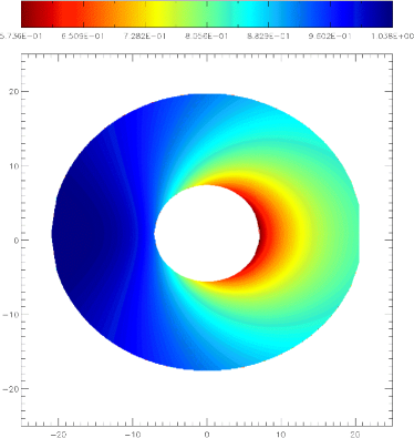
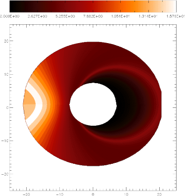
Figure 1: Redshift images (left panel) and flux images (right panel) of the accretion disc on the $\left(\alpha,\beta\right)$ plane for a Schwarzschild black hole and observer with inclination of $30^{\circ}$

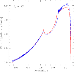
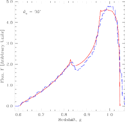
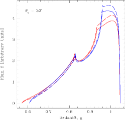
Figure 2: Comparison of the relativistic line profile computed by our model ( red solid line) with that computed by the XSPEC diskline model ( blue dashed line) for $\varepsilon\left(r_{e}\right)\propto r^{-3}$ and $f\left(\mu_{e}\right)=1$ (left panel) and that computed by the XSPEC laor model ( blue dashed line) for $\varepsilon\left(r_{e}\right)\propto r^{-3}$ and $f\left(\mu_{e}\right)\propto\left(1+2.06\mu_{e}\right)$ (middle panel). The right panel shows a comparison of the relativistic line profiles generated by our model with (a) $\varepsilon\left(r_{e}\right)\propto r_{e}^{-3}$, $f\left(\mu_{e}\right)=1$ (solid lines) and (b) $\varepsilon\left(r_{e}\right)\propto r_{e}^{-3}$, $f\left(\mu_{e}\right)\propto\left(1+2.06\mu_{e}\right)$ (dashed lines) for the case of Schwarzschild ( red lines) and maximal Kerr ( blue lines) black holes.

The diskline code assumes a Schwarzschild metric ($a=0$) and additionally that light travels in straight lines (so the angular emissivity term is irrelevant). Hence we use $f(\mu_{e})=1$ (no angular dependance of the emissivity). Figure 1 (left panel) shows our redshift image of the Schwarzschild disc, where the colours indicate the value of the redshift factor, $g$, whilst Figure 1 (right panel) shows the corresponding flux image with each redshift bin coloured by its area on the observers sky. Figure 2 (left panel) shows our line profile compared to that from the diskline code. We see that our new model matches very closely to the XSPEC diskline model for a nearly face on disk. Whilst the key difference between our model and diskline is the inclusion of light-bending effects, this has little effect if there is no angular dependance to the emissivity.

By contrast, the laor code is based on transfer functions calculated by Monte-Carlo methods over a range of radii in extreme Kerr, and includes a standard limb darkening law $f(\mu_{e})\propto(1+2.06\mu_{e})$. We include this limb darkening in our code, and Figure 2 (middle panel) shows the line profile comparison. It is clear that there are some resolution issues in the XSPEC laor model.

The effects of spacetime and emissivity are shown in Fig. 2 (right panel) with radial emissivity of $r^{-3}$ over 6–20 $r_{g}$. The lines are (from top to bottom at the blue peak) from extreme Kerr with limb darkening, extreme Kerr with constant angular emissivity, Schwarzschild with limb darkening and Schwarzschild with constant emissivity. There is a 40% change in relative height in the blue peak between the various models. In data fitting, if the model assumed a Kerr metric with limb darkening (i.e. laor) while the real line was from a Schwarzschild, constant angular emissivity disc, then a $\chi^{2}$ minimisation would tend to match up the blue peak heights. This would result in a deficit across the red wing, pulling the radial emissivity into a more centrally peaked value for $q$. We caution that there are significant uncertainties in the angular distribution of the line emissivity which can change the expected line profile due to lightbending even at low/moderate inclinations.

4 Conclusions

We show results from our code for a disc between 6–20 $r_{g}$ with radial emissivity $\propto r^{-3}$ in both Schwarzschild and Kerr metrics, comparing these with the diskline and laor models in XSPEC. Lightbending is always important, in that the image of the disc at the observer always consists of a range of different emission angles. This means that the angular dependance of the emitted flux can make significant changes to the derived line profile. While calculating the strong gravity effects is a difficult numerical problem, the underlying physics is well known. By contrast, the angular emissivity is an astrophysical problem, and is not at all well known as it depends on the ionisation state of the disc as a function both of height and radius. Figure 2 (right panel) demonstrates the effect of this unknown astrophysics folded through both Schwarzschild and extreme Kerr spacetimes, showing there can be a 20% difference in the ratio of the blue-to-red peak heights simply from the assumed angular emissivity. Before we can use the line profiles to test General Relativity, to probe the underlying physics, we will need to have a much better understanding of the astrophysics of accretion.

References

- [1] Cunningham, C.T.; ApJ, 1975, 202, 788
- [2] Fabian, A.C.; Rees, M.J.; Stellar, L.; White, N. E.; MNRAS 1989, 238, 729.
- [3] Tanaka, Y.; Nandra, K.; Fabian, A. C.; Inoue, H.; Otani, C.; Dotani, T.; Hayashida, K.; Iwasawa, K.; Kii, T.; Kunieda, H.; Makino, F.; Matsuoka, M. Nature, 1995, 375, 659.
- [4] Iwasawa, K.; Fabian, A. C.; Reynolds, C. S.; Nandra, K.; Otani, C.; Inoue, H.; Hayashida, K.; Brandt, W. N.; Dotani, T.; Kunieda, H.; Matsuoka, M.; Tanaka, Y.; MNRAS 1996, 282, 1038.
- [5] Wilms, J rn; Reynolds, Christopher S.; Begelman, Mitchell C.; Reeves, James; Molendi, Silvano; Staubert, R diger; Kendziorra, Eckhard; MNRAS 2001, 328, L27.
- [6] Laor, A.; ApJ 1991, 376, 90.
- [7] Beckwith, Kris; Done, Chris; MNRAS 2004 (submitted) (astro-ph/0402198).