Down-Sizing in Galaxy Formation at $z\sim 1$ in the Subaru/XMM-Newton Deep Survey (SXDS)

Abstract

We use the deep wide-field optical imaging data of the Subaru/XMM-Newton Deep Survey (SXDS) to discuss the luminosity (mass) dependent galaxy colours down to $z^{\prime}$=25.0 (5$\times$10⁹$h_{70}^{-2}$M_⊙) for $z\sim 1$ galaxies in colour-selected high density regions. We find an apparent absence of galaxies on the red colour–magnitude sequence below $z^{\prime}\sim 24.2$, corresponding to $\sim$$M^{*}$+2 ($\sim$10¹⁰M_⊙) with respect to passively evolving galaxies at $z\sim 1$. Galaxies brighter than $M^{*}$$-$0.5 (8$\times$10¹⁰M_⊙), however, are predominantly red passively evolving systems, with few blue star forming galaxies at these magnitudes.

This apparent age gradient, where massive galaxies are dominated by old stellar populations while less massive galaxies have more extended star formation histories, supports the ‘down-sizing’ idea where the mass of galaxies hosting star formation decreases as the Universe ages. Combined with the lack of evolution in the shape of the stellar mass function for massive galaxies since at least $z\sim 1$, it appears that galaxy formation processes (both star formation and mass assembly) should have occurred in an accelerated way in massive systems in high density regions, while these processes should have been slower in smaller systems. This result provides an interesting challenge for modern CDM-based galaxy formation theories which predict later formation epochs of massive systems, commonly referred to as “bottom-up”.

Accepted for publication in MNRAS Main Journal

1 Introduction

Galaxy properties depend strongly on the mass of the system. Based on the 122,808 galaxies drawn from the Sloan Digital Sky Survey (SDSS), Kauffmann et al. (2003) have recently shown an interesting bimodality of local galaxy properties separated at a stellar mass of $\sim$3$\times$10¹⁰M_⊙. In particular, in contrast to massive galaxies which are dominated by old stellar populations showing little sign of recent star formation, less massive galaxies have a much larger contribution from young stars and a significant fraction of these low mass galaxies are likely to have experienced recent starbursts (see also Gavazzi & Scodeggio 1996; Baldry et al. 2004). The morphological signatures also depend on the mass or luminosity, with massive galaxies showing centrally-concentrated light profiles (early-type/bulge morphologies), and less massive galaxies showing less concentrated profiles (late-type/disk morphologies; e.g., Kauffmann et al. 2003; Treu et al. 2003).

Based on the $z\mathrel{\raise 1.50696pt\hbox{$\scriptstyle>$}\kern-6.00006pt\lower 1.72218pt\hbox{{$\scriptstyle\sim$}}}1$ galaxies in the Hawaii Deep Fields, Cowie et al. (1996) have suggested that the most massive galaxies form earliest in the Universe, and star formation activity is progressively shifted to smaller systems, although their data are limited to galaxies brighter than $M^{*}$. They have termed this phenomenon ‘down-sizing’ in star forming galaxies. This apparent age gradient as a function of mass, where the massive galaxies are uniformly old while the less massive galaxies tend to be younger, appears to be at odds with cold dark matter (CDM) models of the Universe. In these models, galaxies form in a ‘bottom-up’ or hierarchical manner, with small systems collapsing first and massive galaxies forming later via the assembly of these small systems.

Motivated by this interesting and fundamental puzzle in galaxy formation, we have chosen to investigate the mass dependence of galaxy properties at high redshift ($z\sim 1$) in more detail by studying much lower mass systems than previous work. To do this, we have used a statistically large sample of galaxies drawn from the Subaru/XMM-Newton Deep Survey (Sekiguchi et al. 2004), which has the unique advantage of depth ($z^{\prime}$=25.2 at 5–8$\sigma$) and width (1.2 deg²) achieved via the wide-field (30’) camera Suprime-Cam on the 8.2-m Subaru Telescope.

Bell et al. (2004) have recently analysed the redshift-dependent colour distributions of $\sim$25000 galaxies over 0.78 deg² based on the COMBO-17 optical survey (Wolf et al. 2003). This survey, however, is $\sim$3 magnitudes shallower than the SXDS, reaching only to $\sim$$M^{*}$ at $z\sim 1$. Our data therefore provides the first opportunity to study the properties of faint galaxies at high redshift.

We adopt the cosmological parameters ($H_{0}$, $\Omega_{m}$, $\Omega_{\Lambda}$)=(70, 0.3, 0.7) throughout this paper, and define $h_{70}$ as $H_{0}$/(70 km s^-1Mpc^-1). With this parameter set, 1 arcmin corresponds to 0.48 Mpc at $z\sim 1$. All the magnitudes in this paper will be given in the AB-magnitude system.

We structure the paper as follows. After an introduction in §1, we briefly describe in §2 the Subaru imaging data upon which the following analyses are based. In §3, we identify the high density regions at $z\sim 1$ by using the red sequence colour slice technique and determine the galaxy demographics in these regions by subtracting off foreground and background contaminations in a statistical manner. We investigate the photometric properties of this statistical sample of $z\sim 1$ galaxies in §4, with particular emphasis on the faint end. A discussion of our results and conclusions are given in §5 and §6, respectively.

2 Observation and Data Reduction

Detailed information on the observations, the data set and the data reduction of the Subaru/XMM-Newton Deep Survey (SXDS) project will be fully described in Sekiguchi et al. (2004) and Furusawa et al. (2004).

Here we only briefly summarise the data on which our analyses are based. The SXDS Field is located at RA=02:18:00, Dec=$-$05:00:00 (J2000). This is a multi-wavelength survey programme being conducted using a range of facilities including Subaru/Suprime-Cam/FOCAS, UKIRT/WFCAM, XMM-Newton, VLA, and JCMT/SCUBA.

As a major part of this survey, we have taken deep Subaru optical images of a 1.2 deg² field using 5 pointings of the wide-field camera, Suprime-Cam (34^′$\times$27^′), which covers most of the coordinated XMM-Newton deep survey fields. We have $B$, $R$, $i^{\prime}$ and $z^{\prime}$-band images for each pointing and the depths are slightly different among the pointings, but go uniformly down to $B\sim 27.4$, $R\sim 26.8$, $i^{\prime}\sim 26.4$ and $z^{\prime}\sim 25.2$ in a 2-arcsec aperture at $\geq$5$\sigma$. The typical seeing sizes in the combined frames are 0.78–0.9^′′.

We have used SExtractor Version 2.2.2 (Bertin & Arnouts 1996) to detect objects in the $z^{\prime}$-band and perform photometry on the sources in all the bands. We use MAGBEST as an estimate of the total $z^{\prime}$ magnitude, and the 1.8^′′ diameter aperture magnitudes to derive colours such as $R-z^{\prime}$ and $i^{\prime}-z^{\prime}$. We exclude stellar objects from our analyses by rejecting sources for which the CLASS_STAR index is larger than 0.8 in the $z^{\prime}$-band image.

Due to concerns that our rejection of compact objects may exclude some low luminosity galaxies at high redshift, which could affect our later discussion of the deficit of faint red galaxies, we have repeated our analysis without performing this star–galaxy separation. We find that there is little effect on the derived colour–magnitude diagram, luminosity function and stellar mass function of $z\sim 1$ galaxies, except for the retention of some obvious stars which are not properly removed in the statistical subtraction process (§3.2). These objects are clearly too blue ($R-z^{\prime}<0.6$) and too bright ($z^{\prime}<21.5$) to be real galaxies at $z\sim 1$. The analyses which follow in this paper are therefore based on the sample of objects with CLASS_STAR$<$0.8.

3 Data Analysis

3.1 Identification of high density regions at $z\sim 1$

In this paper we focus on galaxies at $z\sim 1$, since this is the highest redshift which can be selected and studied in the rest-frame optical spectral regime based solely on our optical imaging observations. To construct a sample of $z\sim 1$ galaxies from our data, we first identify overdense regions at $z\sim 1$ using colour selection criteria and then make a statistical correction for foreground and background contamination using the galaxies from control fields. We describe this technique more in detail below.

We know a priori that clusters of galaxies contain large excesses of red early-type galaxies compared to the averaged field, and that these galaxies show a tight colour–magnitude relationship both locally and at high redshifts (eg., Visvanathan & Sandage 1977; Dressler 1980; Butcher & Oemler 1984; Bower, Lucey & Ellis 1992; Ellis et al. 1997; Stanford et al. 1998; Kodama et al. 1998; van Dokkum et al. 1998). We can therefore search for high density regions at $z\sim 1$ by mapping the galaxies within a narrow colour range around the expected location of the colour–magnitude sequence at that redshift. The high density regions are identified as galaxy clumps on the projected sky after these colour cuts. This technique has been applied successfully by many authors (e.g., Gladders & Yee 2000; Kodama et al. 2001) and recognised as an efficient way of searching for high density systems in the distant Universe.

Figure 1: The colour cuts used for selecting the red $z\sim 1$ galaxies are indicated by the horizontal dot-dashed lines delimiting the ranges $1.7<R-z^{\prime}<2.0$ and $0.8<i^{\prime}-z^{\prime}<1.1$. Three model colour tracks are plotted as a function of redshift from Kodama, Bell & Bower (1999). The red curves show the colour tracks for a passively evolving galaxy formed in an instantaneous burst at $z_{f}$=5 (Kodama et al. 1998). The blue curves indicate the tracks for exponentially decaying star formation with an e-folding time of 5 Gyr and the green curves show the combination of these two models with equal weight in the rest-frame $B$-band luminosity.

Here we use both $R-z^{\prime}$ and $i^{\prime}-z^{\prime}$ colours. As shown in Fig. 1, the red passive galaxies at $z\sim 1$ can be isolated by using the colour slices defined by $1.7<R-z^{\prime}<2.0$ and $0.8<i^{\prime}-z^{\prime}<1.1$. We note that these criteria are expected to produce a sample of galaxies with a range of redshifts $0.9\mathrel{\raise 1.50696pt\hbox{$\scriptstyle<$}\kern-6.00006pt\lower 1.72218pt\hbox{{$\scriptstyle\sim$}}}z\mathrel{\raise 1.50696pt\hbox{$\scriptstyle<$}\kern-6.00006pt\lower 1.72218pt\hbox{{$\scriptstyle\sim$}}}1.1$ which corresponds to the range in distance modulus $\Delta$dm=0.5 mag (0.2 dex). Including the small k- and e-corrections, the $z^{\prime}$-band magnitude can be different by 0.7 mag (0.28 dex) at most. Since we discuss the photometric properties for our colour-selected sample as a whole, it should be noted that the scatter in the red sequence and luminosity and stellar mass functions shown in §4 are expected to be increased by these amounts due to the inclusion of galaxies over a range of redshifts.

Table 1: The $z\sim 1$ high density regions identified in the SXDS field. The relative coordinates are given with respect to the field centre (RA=02:18:00, Dec=$-$05:00:00).

ID	RA (J2000)	Dec (J2000)	dRA	dDec	Note
c1	02:18:08.03	$-$05:01:00	2.0′	$-$1.0′
c2	02:19:24.34	$-$04:51:00	21.0′	9.0′
c3	02:20:00.48	$-$05:09:00	30.0′	$-$9.0′	included due to narrow C-M sequence
c4	02:20:26.58	$-$04:48:30	36.5′	11.5′
c5	02:17:35.90	$-$04:32:00	$-$6.0′	28.0′
c6	02:16:35.70	$-$04:49:30	$-$21.0′	10.5′	excluded due to two bright stars nearby

Figure 2: The 2-D distribution of the 1503 ‘red’ galaxies ($z\sim 1$) in the SXDS field (1.2 deg²) selected by the colour and magnitude cuts shown at the top of the panel. The contours show the local surface density of the red galaxies measured by smoothing the galaxy distribution with a 1.2-arcmin radius Gaussian. The contours show excesses of 2, 3, 4, and 5$\sigma$ above the average density. The large open circles (with a radius of 3 arcmin) indicate the $z\sim 1$ high density regions identified from this map.

Figure 2 shows the 2-D distribution of the red galaxies after the colour cuts were applied. Here we have also limited the galaxies to those brighter than $z^{\prime}=23$ to further contrast the red sequence galaxies against the foreground/background galaxies. We have selected 6 high density regions (c1–c6), each of which has a 3 arcmin radius as indicated by the large circles, and we list these in Table 1. These regions all have a $>$$3\sigma$ excess in surface density, except for the southeast clump (c3) which is detected at only the $2\sigma$ level. Nevertheless, we include this clump since it shows a tight colour–magnitude sequence and is likely to be a physically associated system, although the spatial distribution is a bit sparse. On the other hand, we do not include the c6 region in our further analysis since there are two very bright stars nearby ($<$1–2^′) which are likely to significantly affect the photometry. We show the colour–magnitude diagrams for the five selected regions (c1–c5) in Fig. 3.

Some spectroscopic observations in the SXDS field were made with FOCAS on Subaru in October and December 2003. We obtained spectra for 64 randomly-chosen galaxies from our colour-selected $z\sim 1$ sample with $z^{\prime}<22$. Redshifts were obtained for 59 of these, of which 56 (88% of the entire spectroscopic sample of 64 galaxies) fall within the redshift interval of $0.87\leq z\leq 1.12$. Our colour criteria for selecting $z\sim 1$ red galaxies are therefore shown to be reliable and allow only minor contamination. These results do not allow us to estimate the completeness of our technique, although this is not a concern since we do not discuss, for example, the absolute number density of $z\sim 1$ galaxies in this paper.

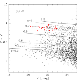
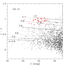
Figure 3: Colour–magnitude diagrams for the galaxies within the 3 arcmin circles of our $z\sim 1$ high density regions (c1–c5). Galaxies with $z^{\prime}<23$ and $1.7<R-z^{\prime}<2.0$ and $0.8<i^{\prime}-z^{\prime}<1.1$, on which the overdensities of the $z\sim 1$ red galaxies are based, are shown as filled circles.

3.2 Statistical field subtraction

Since the spectroscopic data for our $z\sim 1$ galaxies are still very sparse (only $\sim$60 galaxies), and that we can reach only down to $z^{\prime}=23$ in 1–2-hour exposures on Subaru, it is essential to apply a conventional “statistical” field subtraction method to investigate the statistical properties of $z\sim 1$ galaxies, especially for faint ($z^{\prime}>23$) galaxies. To achieve this, we have selected 15 control fields from the SXDS image, each with a 3^′ radius. These fields have been chosen to carefully avoid bright stars, the 6 $z\sim 1$ high density regions (c1–c6), and the 16 foreground cluster candidates which are detected in the XMM-Newton observations as extended X-ray sources (Fig. 4). By combining all these 15 independent fields, we have a good representative sample of the average field population over $\sim$424 arcmin².

Figure 4: The 15 control fields are shown by solid open circles (with a radius of 3 arcmin). These regions are selected to avoid the regions severely affected by bright stars (shown) and the 16 regions of foreground cluster candidates ($0<z<0.8$) where extended X-ray emissions are detected (dotted open circles).

We can then subtract this field sample from the target fields (c1–c5) to isolate the $z\sim 1$ galaxies. This works because both the control and target fields have the same number density of foreground and background galaxies (statistically speaking), since we have not used any information about the foreground/background to select the target fields. To gain better statistics in the field subtraction process, we have combined the five $z\sim 1$ high density regions and discuss the averaged properties throughout the rest of this paper.

The actual field subtraction process depends on what we plot. For example, to construct the luminosity function in our $z\sim 1$ high density regions, we just straightforwardly subtract the magnitude distribution of the galaxies in the control fields from that of the high density regions. In order to plot a colour–magnitude diagram, however, we must do the subtraction in two dimensions using colours and magnitudes at the same time, for which we use the Monte-Carlo technique described in Appendix A in Kodama & Bower (2001). In short, we make grids on the colour–magnitude diagram (in this paper we use bin sizes of $\Delta$($R-z^{\prime}$)=0.15 and $\Delta$$z^{\prime}$=0.4), and count the number of galaxies in each bin in both the control and target fields. We scale the former number to match the smaller area of the target fields, and for each bin we assign a probability that a galaxy in the target fields should be subtracted as a field galaxy. We then generate a random number between 0 and 1 for each galaxy and decide whether it should be removed depending on whether this random number is larger or smaller than the probability. If the probability of being a field galaxy exceeds unity (this happens if the number of galaxies to be subtracted exceeds the available number of galaxies in a certain bin), we re-distribute the excess probability to the neighbouring bins. We apply the same process when producing a $BRz^{\prime}$ colour–colour diagram, where we use bin sizes of $\Delta$($R-z^{\prime}$)=0.15 and $\Delta$($B-z^{\prime}$)=0.37.

The largest potential problem in the statistical field subtraction comes from so-called cosmic variance. Even though we have averaged over the large areas of the control fields and hence have a good statistical sample for the averaged field population, the field-to-field variation in such things as the number density and colour–magnitude distribution still remains in the limited target field to be processed (the combined $z\sim 1$ high density regions comprise a total area of 141 arcmin²). To assess the impact of these field variation on the results presented in this paper, we have divided the control fields into three independent areas, each of which is a combination of five 3^′ circles giving a 141 arcmin² field of view, the same as our combined target fields. We then use these three control samples to perform the statistical field subtraction and measured the scatter in the results. We will discuss the outcome of this process later in §4.3 and Fig. 11, but the effect is found to be small since our target field has relatively a wide area by combining the five regions.

4 Results

4.1 The colour–magnitude and colour–colour diagrams

In Fig. 5, we show the field-corrected colour–magnitude diagram for the $z\sim 1$ galaxies in the combined high density regions (c1–c5). This is a typical Monte-Carlo run for the statistical field subtraction, and $\sim$900 galaxies are left over after the subtraction which are expected to lie in the redshift interval of $0.9\mathrel{\raise 1.50696pt\hbox{$\scriptstyle<$}\kern-6.00006pt\lower 1.72218pt\hbox{{$\scriptstyle\sim$}}}z\mathrel{\raise 1.50696pt\hbox{$\scriptstyle<$}\kern-6.00006pt\lower 1.72218pt\hbox{{$\scriptstyle\sim$}}}1.1$.

From a glance at this diagram, it is obvious that the fraction of blue galaxies is large. We estimate the blue fraction from this diagram using a magnitude cut at $z^{\prime}$=23.2 ($\sim$$M_{V,\rm rest}^{*}$+1) and a blue/red separation at $R-z^{\prime}$=1.3 ($\Delta$($B$$-$$V$)_rest$\sim$0.2), which mimic the original Butcher & Omeler (1984) criteria. We find the blue galaxy fraction to be as high as $\sim$50%, which is twice as large as the one for rich clusters at $z\sim 0.5$ suggested by Butcher & Oemler. These blue galaxies are probably still vigorously forming stars at $z\sim 1$, and in fact if we plot a field-corrected colour–colour diagram (Fig. 6), we find that they follow the expected star formation sequence at $z\sim 1$. A remarkable fact is the complete absence of galaxies in the regions where we expect foreground/background contaminants to lie, which strengthens the reliability of our statistical field correction. For comparison, the colour–magnitude and colour–colour diagrams for galaxies in the control fields are shown in Figs. 7 and 8.

We also notice that the scatter in Fig. 5 around the red colour–magnitude sequence is large. However, we attribute this to the fact that the galaxies span a range of redshifts ($\Delta$$z$$\sim$0.2). In fact, the individual colour–magnitude diagrams of the target fields c1–c5 show tighter red sequences (cf. Fig. 3).

Fig. 5) also shows the highlight of our results, namely the colour distribution of galaxies as a function of luminosity. Specifically, there are two critical magnitudes at $z^{\prime}$=21.7 ($M^{*}-0.5$) and $z^{\prime}$=24.2 ($M^{*}$+2) which separate this diagram into three characteristic magnitude ranges: the brightest end ($z^{\prime}<21.7$) is dominated by red galaxies ($R-z^{\prime}>1.5$), while the faintest end ($z^{\prime}>24.2$) is dominated by blue galaxies ($R-z^{\prime}<1.5$), and between these is the transition region where both red and blue galaxies co-exist. Note that the lower critical magnitude of $z^{\prime}$=24.2 is at least one magnitude brighter than the limit of the data (shown by the vertical dot-dashed line, corresponding to 5–8$\sigma$ detections), assuring $>$10$\sigma$ detections. The $R$-band images are also deep enough to detect the red galaxies (see the slanted dot-dashed line). The deficit of the red faint galaxies we discover is therefore not caused by incompleteness.

These critical magnitudes correspond to 8$\times$10¹⁰M_⊙ and 10¹⁰M_⊙, respectively (we describe how we convert from luminosity to mass in §4.3). Therefore, the most luminous (massive) galaxies are always old while the faintest (least massive) galaxies are young or still forming significant amount of stars, with the transition occurring in between.

Bell et al. (2004) showed from COMBO-17 data (Wolf et al. 2003) that field galaxies display clear bimodal colour distribution at all redshifts $z\mathrel{\raise 1.50696pt\hbox{$\scriptstyle<$}\kern-6.00006pt\lower 1.72218pt\hbox{{$\scriptstyle\sim$}}}1$. At $z\sim 1$, Bell et al. reached only $M^{*}$, which is 2 magnitudes too bright to see the deficit of red faint galaxies. In this paper, our deep imaging data have allowed us to find that the bimodal colour distribution has a strong luminosity dependence at $z\sim 1$. The bimodality is now better described by the existence of two characteristic populations in the colour–magnitude diagram, namely, ‘red + bright’ and ‘blue + faint’ populations. We should note here that Baldry et al. (2004) have recently presented a similar result for the local Universe, based on SDSS data.

Our interesting results on the colour–magnitude distribution of galaxies at high redshift ($z\sim 1$) will be further discussed in the following sections based on the colour-dependent luminosity and stellar mass functions.

Figure 5: Field-corrected colour–magnitude diagram for the $z\sim 1$ galaxies taken from the combined high density regions (c1–c5). This is an example of the Monte-Carlo run and around 900 galaxies are plotted. The solid line shows the expected location of the colour–magnitude sequence at $z=1$ assuming passive evolution since the formation redshift $z_{f}$=5 (Kodama et al. 1998). The dashed curves show lines of constant stellar mass (see §4.3 for details). A deficit of red faint galaxies below $z^{\prime}=24.2$ ($M^{*}$+2, right vertical dotted line) or $M_{\rm stars}$=10¹⁰M_⊙ is clearly seen. Note that this critical magnitude and mass is well above the 5$\sigma$ detection limit shown by the dot-dashed lines.

Figure 6: A colour–colour diagram for the same field-corrected $z\sim 1$ galaxies as were plotted in Fig. 5. The three models plotted here are the same as those in Fig. 1, with redshift increasing from $z$=0 to 2 in a clockwise direction along the curves. The internal reddening vector for $z\sim 1$ star forming galaxies (Calzetti et al. 2000) is shown by an arrow. Most of the galaxies are located along the star forming locus at $z\sim 1$ as shown in the dashed curve, where star formation rate is changing along the curve, although a slight offset is seen possibly due to the internal reddening or model uncertainties.

Figure 7: A colour–magnitude diagram for the combined control fields with the same area size as Fig. 5 for comparison. Nearly 5000 galaxies are plotted.

Figure 8: The same as Fig. 7, but a colour–colour diagram for the combined control fields.

4.2 Luminosity functions

The field-corrected luminosity functions are shown in Fig. 9. The overall shape of the luminosity function for all galaxies is a normal Schechter type although the flattening of the faint end is seen below $z^{\prime}\sim 23$ ($\sim$$M^{*}$+1). It is obvious, however, if the luminosity function is separated into red and blue galaxies at $R-z^{\prime}=1.5$ as shown by the red and blue curves, respectively, they are quite different: the red one has a bell-like (Gaussian) shape and dominates at brighter magnitudes, while the blue one has a much steeper slope and dominates the faint number counts. Moreover, the deficit of red galaxies at the faint end and the deficit of blue galaxies at the bright end that we discussed in the previous subsection are both identified here too. Note that the faintest magnitude plotted here is $z^{\prime}=25$ mag which corresponds to 6–10$\sigma$ in detection to assure good completeness. The raw galaxy number counts also show that the completeness is high at this magnitude (Yamada et al. 2003), which can also be judged from Fig. 7. These colour-dependent luminosity functions look very similar to the local luminosity functions derived from the SDSS data (Blanton et al. 2001).

Kajisawa et al. (2000) claimed a deficit of faint galaxies below $M^{*}$+1.5, including both red and blue galaxies, in the core of the 3C 324 cluster at $z=1.21$ from their deep $K^{\prime}$-band data. However, we do not see such a trend, either in our data (as shown by the solid line in Fig. 9 all the way down to $M^{*}$+3), nor in the data of Kodama & Bower (2003), who presented the $K_{s}$-band luminosity functions of $z\sim 1$ clusters. Nakata et al. (2001) failed to confirm a deficit in the cluster member candidates selected from photometric redshifts in their re-analysis of the 3C 324 cluster. We speculate that the reason why Kajisawa et al. (2000) saw such a deficit of less massive galaxies is because of their limited field coverage (cluster-centric distance $r_{c}$$<$40^′′ or 0.33 Mpc) and hence poor statistics and strong luminosity segregation.

Figure 9: Field-corrected $z^{\prime}$-band luminosity functions for the $z\sim 1$ galaxies. The solid curve shows the total luminosity function, while the dashed and dotted curves show the luminosity functions for red and blue galaxies, respectively, separated at $R-z^{\prime}=1.5$. The error bars shown here are purely Poissonian.

4.3 Stellar mass functions

Since the $z^{\prime}$-band still samples rest-frame optical light longer than the 4000Å break for our $z\sim 1$ galaxies, we can obtain a rough estimate of the stellar mass from the $z^{\prime}$-band luminosity (e.g., Dickinson et al. 2003). To do this, however, we need an estimate of the mass-to-light (M/L) ratio for individual galaxies, which will depend on their star formation histories. In fact the M/L ratio in the observed $z^{\prime}$-band at $z\sim 1$ differs by a factor of $\sim$7–8 between passively evolving galaxies formed at high redshift ($z_{f}$=5) and those galaxies which have formed stars constantly over a long period. Here we use the $R-z^{\prime}$ colour to estimate the M/L ratio in the same way as Kodama & Bower (2003). In short, we take the relation between $R-z^{\prime}$ and M/L ratio at $z=1$ for models representing a sequence of galaxies with different ratios of bulge to total mass (Kodama, Bell & Bower 1999), where a disk component is added to the underlying passively evolving bulge component. We then use Kennicutt’s (1983) initial mass function (IMF) to scale the stellar mass. The resultant field-corrected stellar mass functions of galaxies at $z\sim 1$ are shown in Fig. 10. Again, the deficit of blue massive galaxies and the deficit of red less massive galaxies are clearly seen.

The error bars already include the Poisson noise inherent in the limited number statistics and the statistical field subtraction. However, the field subtraction process may also suffer from cosmic variance where galaxy distribution are known to be non-uniform both locally and at high redshifts (e.g., Peacock et al. 2001; Kodama et al. 2001; Shimasaku et al. 2003). Therefore it is essential to cover as wide a field as possible in order to average out the field-to-field variations. The wide field coverage of our data (i.e., 1.2 deg², corresponding to the co-moving volume of 2.1$\times$10⁶ Mpc³ within $0.9\leq z\leq 1.1$) helps us in this respect. This also allows us to estimate the effect of field-to-field variations on $\sim$10 Mpc scales in the derived stellar mass function within our data. To achieve this, we take three different and independent sets of control fields, each consisting of five circled areas with $3^{\prime}$ radii, giving 141 arcmin² each. This is the same area as the combined high density regions from which our $z\sim 1$ galaxies are extracted (see also §3.2). Changing the control field populations among these three independent samples when we perform the field subtraction therefore gives us an estimate of the internal field-to-field variation on our results. As shown in Fig. 11, the effect is small and typically comparable to the pure Poisson errors shown in Fig. 10. The deficits of massive blue galaxies and smaller red galaxies are still significant, and we conclude that field-to-field variation among our control fields is not a critical issue in our analyses.

It is also interesting to examine the evolution of the stellar mass functions with redshift since this provides a critical test for the CDM-based bottom-up scenario for galaxy formation and evolution (e.g., Kauffmann & Charlot 1998; Baugh et al. 2002). In Fig. 12, our total stellar mass function (blue filled circles) is compared to previous measurements of the stellar mass function at $z\sim 1$ and $z\sim 0$. All the curves and data points have been normalised at 5$\times$10¹⁰M_⊙ to have the same amplitude as the 2dF mass function. The agreement with the stellar mass function of $z\sim 1$ cluster galaxies based on near-infrared imaging (Kodama & Bower 2003) is remarkable, which suggests that we are indeed looking at high density regions at $z\sim 1$ in this study. If we compare the observed stellar mass functions at $z\sim 1$ to their lower redshift counterpart (e.g., 2MASS clusters; Balogh et al. 2001), we see the lack of evolution from $z\sim 1$ to the present-day, as discussed in detail by Kodama & Bower (2003) (see also Kodama et al. 2004 for extension to even higher redshift of $z\sim 1.5$). There are very massive galaxies ($>$10¹¹M_⊙) already in place in high density regions at $z\sim 1$, which must therefore have been assembled even earlier. The rapid mass assembly of these large galaxies is contrasted to the semianalytic model predictions of Nagashima et al. (2002) which shows a much slower mass assembly for cluster galaxies between $z=1$ and $z=0$ (blue dashed and red dotted lines in Fig. 12, respectively).

A deviation can be seen at the faint end between the local clusters (2MASS) and the $z\sim 1$ high density regions (this work and Kodama & Bower 2003) where the slope is flatter in the high-$z$ systems. However, the faint end slope of the 2MASS clusters is only poorly determined (Balogh et al. 2001), and we do not discuss this issue further.

Figure 10: Field-corrected stellar mass functions for the $z\sim 1$ galaxies. The solid curve shows the total mass function, while dashed and dotted curves show the mass functions for red and blue galaxies, respectively, separated at $R-z^{\prime}=1.5$. The error bars shown here are purely Poissonian, and the errors due to field-to-field variation are shown later in Fig. 11.

Figure 11: Effect of field-to-field variation in the derived stellar mass functions, estimated by taking three different sets of control fields. The upper and the lower ends of the vertical error bars show the maximum and the minimum cases while the central dots indicates the average of the three cases. The meaning of the curves is the same as in Fig. 10.

Figure 12: Comparison of our stellar mass functions (blue filled circles with error bars) with other data and models. The $z\sim 1$ cluster data (open triangles) are reproduced from Kodama & Bower (2003) and the 2MASS local cluster data (solid curve) are taken from Balogh et al. (2001). The 2dF field data (open squares) are taken from Cole et al. (2000). The model predictions by the Mitaka semi-analytic model (Nagashima et al. 2002) are shown for $z=0$ (dotted curve) and $z=1$ (dashed curve). These predictions are made for cluster galaxies taken from dark haloes whose circular velocities are larger than 1000 km/s. The observed data and the models are all normalised at 5$\times$10¹⁰M_⊙ to have the same amplitude as the 2dF mass function.

5 Discussion

5.1 Down-sizing in galaxy formation

The most important result shown in this paper is that galaxy formation processes, both mass assembly and star formation, take place rapidly and are completed early in massive systems, while in the less massive systems, these processes (at least star formation) are slower. This ‘down-sizing’ in galaxy formation was first noted by Cowie et al. (1996) who observed that the maximum luminosity of galaxies hosting star formation decreases with decreasing redshift at $z\mathrel{\raise 1.50696pt\hbox{$\scriptstyle>$}\kern-6.00006pt\lower 1.72218pt\hbox{{$\scriptstyle\sim$}}}1$, although their data (from the Hawaii Deep Fields) were limited to galaxies brighter than $<M^{*}$ (see also Pozzetti et al. 2003; Kashikawa et al. 2003; Poggianti et al. 2004; Tran et al. 2004).

Kodama & Bower (2001) investigated the magnitude dependent evolution of cluster galaxies from intermediate redshifts $0.2\mathrel{\raise 1.50696pt\hbox{$\scriptstyle<$}\kern-6.00006pt\lower 1.72218pt\hbox{{$\scriptstyle\sim$}}}z\mathrel{\raise 1.50696pt\hbox{$\scriptstyle<$}\kern-6.00006pt\lower 1.72218pt\hbox{{$\scriptstyle\sim$}}}0.4$ (CNOC clusters, Yee et al. 1996) to the present day (Coma cluster, Terlevich et al. 2001) by letting the distant clusters evolve forward in time by truncating the star formation in blue galaxies. This simulation showed that the less massive galaxies seen today had a higher fraction of blue galaxies in the past compared to the massive galaxies, although the data were complete only to $\sim$$M^{*}$+1. The Butcher–Oemler effect (Butcher & Oemler 1984 show a systematic decrease of blue galaxy fraction above $M_{V}=-20$ with decreasing cluster redshift) can then be partly explained by the down-sizing in star forming galaxies. If these blue galaxies fade and become red quickly after ceasing star formation, they will enter the faint end of the red colour–magnitude sequence. If star formation is truncated from massive galaxies towards less massive galaxies as time progresses, the fraction of blue galaxies brighter than a certain magnitude limit should decrease with time, in line with observations (Bower, Kodama & Terlevich 1998; Kodama & Bower 2001). As the blue galaxies with brighter luminosities stop their star formation, they will evolve to redder colours and fainter magnitudes along the iso-mass lines shown by the dashed lines in Fig. 5, and the faint-end of the red sequence where we see a deficit of galaxies at $z\sim 1$ will be populated with galaxies. This is important because such a deficit of red galaxies between $M^{*}$+2 and $M^{*}$+3 is not seen locally, at least not in the Coma cluster (Terlevich et al. 2000).

We have discussed a significant gradient in age or star forming activity as a function of galaxy luminosity or mass. For clarity, however, we note that our results are not inconsistent with those of Kodama et al. (1998), who discussed a lack of age gradient for cluster early-type galaxies, since they studied only morphologically-selected early-type galaxies brighter than $M^{*}$+1. Furthermore, once star formation has terminated, the blue galaxies would quickly fade and redden and the luminosity weighted age would hardly change along the red colour–magnitude sequence (Kodama & Bower 2001).

What can cause this down-sizing, which is apparently at odds with the ‘bottom-up’ scenario that is a natural consequence of CDM models. Biased galaxy formation (e.g., Cen & Ostriker 1993), in which massive galaxies form from the highest peaks in the initial density fluctuation field, may help to solve this apparent contradiction. The densest fluctuations collapse earlier and hence galaxy formation, both mass assembly and star formation, takes place in an accelerated way in these globally biased regions, while the less massive galaxies seen at $z\sim 1$ collapse later on average since they formed from isolated peaks with lower density. However, a further puzzle is how to keep the star formation rate low so that it continues for long enough to still produce blue galaxies at $z\sim 1$. Two possible mechanisms have so far been proposed to explain this. One suggestion is that the UV background may penetrate into small systems to keep them ionized and prevent star formation (Babul & Rees 1992; Kitayama et al. 2001). The other idea is that supernova explosions cause a periodic gas outflow and re-inflow of gas from the shallow potential well over a long period of time (e.g., Dekel & Silk 1986). Yet no theory can explain, either quantitatively or even qualitatively, the ‘down-sizing’ in galaxy formation, and this is a big challenge for theorists working in this field.

From the observational side, it would be extremely interesting to directly measure the evolution in the break mass with time (cf. Kodama & Bower 2001). Kauffmann et al. (2003) and Baldry et al. (2004) find a break mass of $\sim$2$\times$10¹⁰M_⊙ in the local Universe (SDSS), which is roughly the same break mass as we find at $z\sim 1$. However, in this paper we have discussed only the high density regions, whereas the local analyses are based on the averaged field properties. A direct comparison is therefore not meaningful since galaxy properties are strongly dependent on environment in the sense that galaxy formation and evolution processes are accelerated in high density regions (e.g., Dressler et al. 1980; Kodama et al. 2001; Gomez et al. 2003; Balogh et al. 2004). In fact, extending the deep colour–magnitude analyses of galaxies of this kind along the environmental axis is important since we expect to see a higher break mass in lower density environments due to slower galaxy evolution. It is also appealing to extend this analysis to even higher redshifts ($z\gg 1$) where deep near infrared surveys are essential. With the upcoming wide-field near infrared cameras such as MOIRCS (4^′$\times$7^′) on Subaru and WFCAM (51$\times$51 arcmin² by four pointings) on UKIRT, we will be able to probe the era where massive galaxies are in the process of formation.

6 Conclusions

In this paper, we have presented a photometric analysis of galaxies in colour-selected high density regions at $z\sim 1$, constructed from the unique deep ($z^{\prime}$=25, 6–10$\sigma$) and wide (1.2 deg²) optical multi-colour imaging data taken as a part of the Subaru/XMM-Newton Deep Survey (SXDS) project. Our analysis has been based primarily on the field-corrected colour–magnitude diagram and the colour-dependent stellar mass functions.

Benefitted by the depth of the survey, we have found a deficit of faint red galaxies along the colour–magnitude sequence below $M^{*}$+2 with respect to the passive evolution, or $\sim$10¹⁰M_⊙. Almost all galaxies below this luminosity/mass at $z\sim 1$ are still undergoing significant star formation. The luminous/massive end ($<$$M^{*}$$-$0.5), however, is dominated by old red systems with almost no blue galaxies. The clear distinction of the ‘red + bright’ and ‘blue + faint’ populations at $z\sim 1$ on the colour–magnitude diagram suggests the existence of ‘down-sizing’ in galaxy formation, where star formation is switched off from the massive systems towards the less massive ones as the Universe ages. We find that the mass assembly process is also largely complete by $z\sim 1$ in the high density regions. How to accommodate this down-sizing phenomena in galaxy formation within the context of the bottom-up scenario of the CDM Universe is an interesting puzzle.

References

- [] Babul, A., Rees, M. J., 1992, MNRAS, 255, 346
- [] Baldry I. K., Glazebrook, K., Brinkmann, J., Ivezic, Z., Lupton, R. H., Nichol, R. C., Szalay, A. S., 2004, ApJ, 600, 681
- [] Balogh, M. L., Christlein, D., Zabludoff, A. I., Zarisky, D., 2001, ApJ, 557, 117
- [] Balogh, M. L., et al., 2004, MNRAS, 348, 1355
- [] Baugh, C. M., Benson, A. J., Cole, S., Frenk, C. S., Lacey, C., 2003, in The Mass of Galaxies at Low and High Redshifts, eds., R. Bender, A. Renzini, p. 91.
- [] Bell, E. F., et al, 2004, ApJ, inpress
- [] Bertin, E., Arnouts, S., 1996, A&AS, 117, 393
- [] Blanton, M. R., et al., 2001, AJ, 121, 2358
- [] Bower, R. G., Kodama, T., Terlevich, A., 1998, MNRAS, 299, 1193
- [] Bower, R. G., Lucey, J. R., Ellis, R. S., 1992, MNRAS, 254, 601
- [] Butcher, H., Oemler, A., 1984, ApJ, 285, 426
- [] Calzetti, D., Armus, L., Bohlin, R. C, Kinney, A. L., Koornneef, J., Storchi-Bergmann, T., 2000, ApJ, 533, 682
- [] Cen, R., Ostriker, J. P., 1993, ApJ, 417, 415
- [] Cole, S., Lacey, C. G., Baugh, C. M., Frenk, C. S., 2000, MNRAS, 319, 168
- [] Cowie, L. L., Songaila, A., Hu, E. M., Cohen, J. G., 1996, AJ, 112, 839
- [] Dekel, A., Silk, J., 1986, ApJ, 303, 39
- [] Dickinson, M. Papovich, C., Ferguson, H. C., Budavari, T., 2003, ApJ, 587, 25
- [] Dressler, A., 1980, ApJ, 236, 351
- [] Ellis, R. S., Smail, I., Dressler, A., Couch, W. J., Oemler, A., Butcher, H., Sharples, R. M., 1997, ApJ, 483, 582
- [] Furusawa, H., et al., 2004, in preparation
- [] Gavazzi, G., Scodeggio, M., 1996, A&A, 312, L29
- [] Gladders, M. D., Yee, H. K. C., 2000, AJ, 120, 2148
- [] Gomez, P. L., et al., 2003, ApJ, 584, 210
- [] Kajisawa, M., et al., 2000, PASJ, 52, 53
- [] Kashikawa, N., et al., 2003, ApJ, 125, 53
- [] Kauffmann, G., Charlot, C., 1998, MNRAS, 297, 23
- [] Kauffmann, G., et al., 2003, MNRAS, 341, 54
- [] Kennicutt, R. C., Jr., 1983, ApJ, 272, 54
- [] Kitayama, T., Susa, H., Umemura, M., Ikeuchi, S., 2001, MNRAS, 326, 1353
- [] Kodama, T., Arimoto, N., Barger, A. J., Aragón-Salamanca, A., 1998, A&A, 334, 99
- [] Kodama, T., Bell, E. F., Bower, R. G., 1999, MNRAS, 302, 152
- [] Kodama, T., Bower, R. G., 2001, MNRAS, 321, 18
- [] Kodama, T., Bower, R. G., 2003, MNRAS, 346, 1
- [] Kodama, T., Bower, R. G., Best, P. N., Hall, P. B., Yamada, T., Tanaka, M., 2004, to appear in the Proceedings of the ESO/USM/MPE Workshop on ”Multiwavelength Mapping of Galaxy Formation and Evolution”, astro-ph/0312321
- [] Kodama, T., Smail, I., Nakata, F., Okamura, S., Bower, R. G., 2001, ApJ, 562, L9
- [] Nagashima, M., Yoshii, Y., Totani, T., Gouda, N., 2002, ApJ, 578, 675
- [] Nakata F., Kajisawa, M., Yamada, T., Kodama, T., Shimasaku, K., Tanaka, I., 2001, PASJ, 53, 1139
- [] Peacock, J. A., et al., 2001, 410, 169
- [] Poggianti, B. M., Bridges, T. J., Komiyama, Y., Yagi, M., Carter, D., Mobasher, B., Okamura, S., Kashikawa, N., 2004, ApJ, 601, 197
- [] Pozzetti, L., et al., 2003, A&A, 402, 837
- [] Sekiguchi, K., et al., 2004, in preparation
- [] Shimasaku, K., et al., 2003, ApJ, 568, L111
- [] Stanford, S. A., Eisenhardt, P. R., Dickinson, M., 1998, ApJ, 492, 461
- [] Terlevich, A. I., Caldwell, N., Bower, R. G., 2001, MNRAS, 326, 1547
- [] Tran, K.-V. H., Franx, M., Illingworth, G., Kelson, D. D., van Dokkum, P., 2004, ApJ, in press
- [] Treu, T., Ellis, R. S., Kneib, J.-P., Dressler, A., Smail, I., Czoske, O., Oemler, A., Natarajan, P., 2003, ApJ, 591, 53
- [] van Dokkum, P. G., Franx, M., Kelson, D. D., Illingworth, G. D., Fisher, D., Fabricant, D., 1998, ApJ, 500, 714
- [] Visvanathan, N., Sandage, A., 1977, ApJ, 216, 214
- [] Wolf, C., Meisenheimer, K., Rix, H.-W., Borch, A., Dye, S., Kleinheinrich, M., 2003, A&A, 401, 73
- [] Yamada, T., et al., 2003, in preparation
- [] Yee, H. K. C., Ellingson, E., Carlberg, R. G., 1996, ApJS, 102, 269