Synthetic stellar populations: single stellar populations, stellar interior models and primordial proto-galaxies
Abstract
We present a new set of stellar interior and synthesis models for predicting the integrated emission from stellar populations in star clusters and galaxies of arbitrary age and metallicity. This work differs from existing spectral synthesis codes in a number of important ways, namely (1) the incorporation of new stellar evolutionary tracks, with sufficient resolution in mass to sample rapid stages of stellar evolution; (2) a physically consistent treatment of evolution in the HR diagram, including the approach to the main sequence and the effects of mass loss on the giant and horizontal-branch phases. Unlike several existing models, ours yield consistent ages when used to date a coeval stellar population from a wide range of spectral features and colour indexes. We use Hipparcos data to support the validity of our new evolutionary tracks. We rigorously discuss degeneracies in the age-metallicity plane and show that inclusion of spectral features blueward of 4500 Å suffices to break any remaining degeneracy and that with moderate spectra (10 per 20Å resolution element) age and metallicity are not degenerate. We also study sources of systematic errors in deriving the age of a single stellar population and conclude that they are not larger than %. We illustrate the use of single stellar populations by predicting the colors of primordial proto-galaxies and show that one can first find them and then deduce the form of the IMF for the early generation of stars in the universe. Finally, we provide accurate analytic fitting formulas for ultra fast computation of colors of single stellar populations.
keywords:
galaxies: stellar populations; stars: stellar evolution1 Introduction
The synthetic stellar spectrum of a galaxy is a well established theoretical tool for investigating the properties of the integrated light from distant galaxies where individual stars cannot be resolved. Since the late 60’s several groups have developed different grids of synthetic stellar population models using a variety of stellar interior tracks and observed or theoretical stellar spectra (e.g. Tinsley (1968); Barbaro & Bertelli (1977); Renzini (1981); Bruzual (1983); Barbaro & Olivi (1986); Arimoto & Yoshii (1987); Guiderdoni & Rocca-Volmerange (1987); Bruzual & Charlot (1993); Worthey (1994); Bressan et al. (1994); Fioc & Rocca-Volmerange (1997); Jimenez et al. (1998); Lee et al. (2002)). The idea is very simple: stars are born with a given initial mass function (IMF) and they evolve in time according to stellar evolution. At any time one can compute the integrated spectrum by summing up the individual spectra of the stars in the population at that instant. Two major approaches have been used to compute the integrated light of a stellar population: the fuel consumption theorem (Renzini, 1981; Renzini & Buzzoni, 1983) and the isochrone technique, first developed by Barbaro & Bertelli (1977) and later used by Charlot & Bruzual (1991). The fuel consumption theorem simply uses the fact that the contribution of stars in any post main–sequence evolutionary stage is proportional to the amount of nuclear fuel they burn at that stage, and approximates the post main–sequence evolution of the stars in the integrated population by the stellar track of the most massive star alive at the main sequence turn–off (MSTO). In contrast, the isochrone technique uses a continuous distribution of stellar masses, and hence tracks, to compute the locus in luminosity and at a given time for any mass. From this, a smooth isochrone can be computed. The fuel consumption theorem remains an elegant method of studying the fastest stages in the evolution of any population. On the other hand, with the new generation of fast computers, the isochrone technique is clearly the most accurate and precise method of computing the integrated light of any stellar population.
Regardless of the computational technique used to calculate the integrated spectrum of a stellar population, the most important ingredient remains the stellar input: both stellar interior and stellar atmospheric models. Disagreement over stellar interior models (convection, mass loss, opacities), the modelling of post main sequence evolutionary stages and the modelling of stellar atmospheres (opacities, NLTE effects, bolometric correction, mass loss, etc.), combine to make the derived age of even a simple (i.e., no dust, no AGN contamination) stellar population vary by about 10% (for a fixed mass and metallicity), depending on which of the currently available synthetic stellar population codes (e.g. Charlot et al. (1996); Spinrad et al. (1997)) is used to interpret the data (see section 4). A similar problem occurs when trying to date Globular Clusters in the Galaxy, the age of which is currently uncertain by about 10% (Chaboyer, 1995; Jimenez et al., 1996; Chaboyer & Krauss, 2002).
We have been motivated to attempt to improve this situation by the fact that the new generation of large 8-10m telescopes can now deliver spectra of galaxies at of sufficient quality to merit accurate age dating. The accurate determination of the ages of high-redshift galaxies can yield important constraints not only on models of galaxy formation, but also on the age of the universe. In particular, in a series of papers (Dunlop et al., 1996; Spinrad et al., 1997; Nolan et al., 2001; Nolan et al., 2003) we have addressed the issue of determining the ages of the reddest known elliptical galaxies at . To aid in the interpretation of our data and others, we have developed a set of simple synthetic stellar population models (SSP) that overcomes some of the problems described above.
Most of the disagreement between the existing synthetic stellar evolution codes stems from the difficulty of modelling accurately the post main-sequence evolution, both because the physics involved in these stages is not completely known (opacities, convection, nuclear rates) and because mass loss strongly controls the final fate of the evolution of the star in these phases. Ideally, one would like to have a robust set of stellar models that are computed self-consistently (i.e. interior, photosphere and chromosphere computed at the same time) and that include the effects of mass loss and dust grain formation. However this is not yet possible, and in any case it is important to realise that mass loss cannot be incorporated as a fixed quantity for all stars in the population since it varies from star to star.
In the new synthetic stellar population models presented here we have endeavoured to improve the ability of the modelling to accurately reproduce the post-main sequence evolution of real stellar populations by incorporating an algorithm which has been previously applied with success to a number of other stellar evolution problems (e.g. Jorgensen (1991); Jorgensen & Thejll (1993); Jimenez et al. (1996); Jorgensen & Jimenez (1997)). This algorithm accurately simulates the evolution of all post main-sequence evolution stages, and includes a proper modelling of the HB along with an accurate account of the formation of carbon stars on the AGB. Furthermore, the mixing length parameter and the mass loss are properly calibrated using the position of the RGB and the morphology of the HB in real star clusters, respectively.
The other main new feature of our spectral synthesis models is the incorporation of new stellar evolutionary tracks, with sufficient resolution in mass to sample rapid stages of stellar evolution. As a result of these improvements (which we describe in detail in this paper), unlike several existing population codes, our models yield consistent ages when used to date a coeval population from a wide range of spectral features and colour indexes.
Our new SSP code has been applied successfully to a variety of different populations. it has been used to determine the ages of high redshift galaxies (Dunlop et al., 1996), the ages of Low Surface Brightness Galaxies (Padoan et al., 1997; Jimenez et al., 1998), the role of star formation and the Tully-Fisher law (Heavens & Jimenez, 1999) and the age of the Galactic disc (Jimenez et al., 1998). The purpose of this paper is to present the new library of synthetic stellar population spectra and discuss in more detail the physics and assumptions in our SSP modelling procedure.
The paper is organised as follows: in §2 we present the new set of stellar interior tracks and discuss their accuracy when confronted with individual stellar observations. The synthesis models are presented in §3. The degeneracies in the age-metallicity plane are discussed in §4 while systematic errors are considered in §5. The application of synthesis models to primordial proto–galaxies is presented in §6 along with a method to determine the initial mass function of these galaxies. §7 discusses the IR flux density and detectability of primordial proto–galaxies. Our conclusions are presented in §8. An appendix provides fitting formulas for computing broad band colors of SSPs.
2 Stellar models and physics input
2.1 Library of stellar interiors
We have computed a new interior stellar library with the stellar evolution code JMSTAR developed by one of us (JM) from the code of Eggleton (1971, 1972).
In this code, the whole star is evolved by a relaxation method without use of separate envelope calculations. Some of the advantages of this approach are that (1) gravothermal energy generation terms are automatically included for the stellar envelope, (2) mass loss occurs at the stellar surface rather than an interior point of the star, and (3) the occurrence of convective dredge-up of elements produced by nucleosynthesis in the interior to the photosphere is clearly identifiable. The code uses an adaptive mesh technique similar to that of Werley et al. (1984). Advection terms are approximated by second-order upwind finite differences. Convective energy transport is modeled by using the mixing-length theory described by Mihalas (1978). Composition equations for H, 3He, 4He, 12C, 14N, 16O, and 24Mg are solved simultaneously with the structure equations. Composition changes due to convective mixing are modeled in the same way as Eggleton (1972) by adding diffusion terms to the composition equations. However, the prescription for the diffusion coefficient differs from that of Eggleton (1972). The diffusion coefficient is consistent with mixing-length theory (Iben & MacDonald, 1995), , where is the convective velocity, is the mixing length, and is a dimensionless convective mixing efficiency parameter. OPAL radiative opacities (Iglesias & Rogers, 1996) are used for temperatures (in kelvins) above . For temperature below , we use opacities kindly supplied by D. Alexander and calculated by the method of Alexander & Ferguson (1994). Between these temperature limits, we interpolate between the OPAL and Alexander opacities. Nuclear reaction rates are taken from Angulo et al. (1999) with screening corrections from Salpeter & van Horn (1969) and Itoh et al. (1979). Neutrino loss rates are from Beaudet et al. (1967) with modifications for neutral currents (Ramadurai, 1976). Plasma neutrino rates are from Haft et al. (1994). The equation of state is determined by minimization of a model free energy (see, e.g., Fontaine et al. (1977)) that includes contributions from internal states of the molecule and all the ionization states of H, He, C, N, O, and Mg. Electron degeneracy is included by the method of Eggleton et al. (1973). Coulomb and quantum corrections to the equation of state follow the prescription of Iben et al. (1992), with the Coulomb free energy updated to use the results of Stringfellow et al. (1990). Pressure ionization is included in a thermodynamically consistent manner by use of a hard-sphere free-energy term.
Mass loss is included by using a scaled Reimers (1975) mass-loss law,
| (1) |
for cool stars (T K) and an approximation to the theoretical result of Abbott (1982),
| (2) |
for hot stars ( K). For AGB stars we also include additional mass loss at a rate obtained by fitting the observed mass loss rates for Mira variables (Knapp et al., 1998).
| (3) |
The surface boundary condition is treated as follows. We assume that the atmosphere is plane-parallel and thin. A small value of optical depth (typically ) is assigned to the center of the outermost zone of the stellar model. The corresponding surface temperature is related to the effective temperature, , by the Eddington approximation . The surface gas pressure satisfies where is the effective gravity (surface gravity reduced by the effects of radiation pressure) at the surface of the star. We stress that the code treats the surface boundary on an equal footing with all other shells in the star.

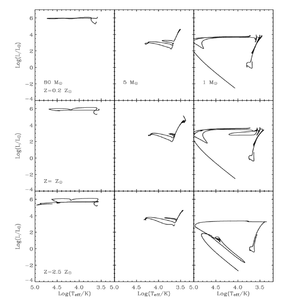
We have used the evolution code to create a grid of interior models with the following parameters. We computed stellar tracks for five different (solar scaled) metallicities: and . We fixed the helium content for the solar model () as to reproduce the luminosity of the Sun at the present age and adopted , consistent with the findings of Jimenez et al. (2003). We show some representative stellar tracks in fig 1 for different metallicities. The tracks were evolved from an initial Hayashi phase to the very late stages in a continuous run. Thus it was possible to deal with the different flashes along the evolution during the giant phases. The evolution of low mass stars () is ended after they settle onto the white dwarf cooling sequence. The evolution of massive stars () is stopped at the end of carbon burning or if the central temperature exceeds . For the intermediate mass stars, the calculation is stopped once the envelope begins to be ejected hydrodynamically due to the radiative luminosity exceeding the local Eddington limit.
| 0.0002 | 0.235 |
| 0.004 | 0.24 |
| 0.01 | 0.25 |
| 0.02 | 0.27 |
| 0.05 | 0.33 |
In order to produce a model for the synthetic stellar population it is necessary to have a set of stellar interior tracks that includes all stellar evolutionary stages for a large range of masses. It is well known that the main discrepancies between different stellar population codes arise from the different treatment of the late stages of stellar evolution (Charlot et al., 1996). Since a proper and accurate modelling of the HB and AGB is extremely important for predicting the UV (HB) and IR (AGB) properties of any stellar population, we have included in our SSP code an accurate semi-empirical algorithm for computing the evolution of the HB and AGB. This is very important since evolution after the RGB cannot be described on the basis of one choice of mass loss parameter (this would result in the absence of a HB in globular clusters). The analytical description of the effect of mass loss (and the influence of different choices of mixing length) in our semi-empirical algorithm, makes it particular useful in handling realistic population descriptions where variation from star to star in the mass loss efficiency needs to be described as a distribution function. We therefore believe that we can obtain the highest accuracy by use of a semi-empirical algorithm. A direct comparison between the semi-empirical method and tracks computed with JMSTAR can be found in Jimenez et al. (1995). The fast and accurate computation of the HB, AGB and TP-AGB, allowed by the semi-empirical method makes it possible to produce stellar tracks for several values of the mass loss parameter ( in the Reimers formulation, or any other similar) and mixing-length parameter (). Therefore, it is possible to analyse the impact of these (unknown) parameters in the final stellar track (see Fig. 2). In two previous studies (Jorgensen & Thejll, 1993; Jimenez et al., 1996) we demonstrated that the morphology of the HB is due to star-to-star variations in the mass loss parameter. This automatically gives a powerful tool to model the HB including, a priori, a realistic distribution of values for the mass loss parameter in the RGB.
Mass loss takes place at the very end of the RGB and is most often described by the empirical Reimers mass loss law Reimers (1975) which is derived from measurements of M type giants. However, instead of following the evolution along the RGB using a fixed value for the parameter (as is usually done in the literature, and as was done by Reimers himself) we proceed in a different way. We use the computed grid of stellar interior models and calculate interpolation formulas (for the RGB) for , , , (core mass), , and (mixing length). The fitting formulas can be found in Jimenez et al. (1996) and for brevity we will not repeat them here. The average value of is determined by matching the observed HB mass distribution. A very fast and accurate numerical computation of the evolution along the RGB can then be performed by taking advantage of the fitting formulas. The addition of mass to the core during a given time step in the integration along the RGB is determined on the basis of the instantaneous luminosity, the known energy generation rate, and the length of the time step. The mass of the core () at the end of the time step determines the new value of according to the fitting formulas. The total stellar mass at the end of each time step is calculated as the mass at the beginning of the time step minus the mass loss rate times the length of the time step. The evolution of the synthetic RGB track is stopped when reaches the value determined in the fitting formulas for the He-core flash. A more detailed study of this approach and its comparison with other stellar models can be found in Jimenez et al. (1995).
Evolution along the AGB is much faster than the corresponding evolution in the RGB and HB, lasting around years. It has two differentiated phases: the early AGB (E-AGB) and the TP-AGB. The E-AGB occurs after the helium core is completely converted to oxygen (and smaller amounts of carbon) and starts when the star is burning helium in a hydrogen-exhausted shell. This phase ends when the hydrogen shell has passed through a minimum in luminosity. The TP-AGB consists of a phase of double-shell burning with thermal-shell flashes and strong mass loss. The modelling of the AGB evolution is rather complicated due to the above considerations. We have modelled it using the prescriptions in Jorgensen (1991) and will not repeat them here. The most important issue is that we can compute when (or not) the star along its AGB will become carbon rich as well as whether the star will end the AGB as a planetary nebula or not. The advantage of this approach to modelling the AGB is that, as for the HB, we can produce accurate predictions on the fate of the star and explore a large range of parameters for the mass loss, mixing length, chemical composition, etc, in a fast and accurate way. The interpolation formulas are based on numerical AGB computations from JMSTAR, as described in Jorgensen (1991), and the evolution is terminated when the core mass reaches the total mass of the star, or the total mass minus the mass of a planetary nebula.

To summarize, the most important advantages of our method for isochrone synthesis are as follows:
-
•
A state-of-the art code to generate stellar interiors that can evolve the stellar track from the initial contracting gaseous phase to the final stages without interruption and that includes the latest advances in reaction rates and opacities.
-
•
A realistic distribution function for the mass loss efficiency parameter is determined on the basis of the HB morphology. The actual values of used in the present work are taken from our previous studies of globular clusters Jimenez et al. (1996). In particular, this distribution ensures a realistic integrated value of the blue and UV radiation from the SSP.
-
•
The mixing-length parameter is determined from fits to globular clusters with known metallicities. This is very important for a realistic description of the red and IR radiation from the SSP models.
-
•
The semi-empirical algorithm has the same accuracy as the original numerical computations on which it is based (plus being improved in and based on observations), but it is computationally much faster.
In order to illustrate the effect that changes in mass loss can have, we have computed, using the above prescription, the evolution of the Sun () with and without mass loss (using the Reimers formalism with ). In the first case the star evolves well into the AGB and develops into a carbon star before it will eventually transform through the post-AGB phase into a WD. In the second case the star leaves the AGB at a much lower luminosity (10 times lower) and at a greater (3000K instead of 2500K). The consequence for synthetic stellar population models are quite obvious: if mass loss is ignored the red-IR luminosity of the population is overestimated (see Fig. 2).
Stellar isochrones are computed by interpolating stellar tracks at equivalent stellar evolutionary points as defined by Schaller et al. (1992). This is important in order to have a good sampling of all stellar evolutionary stages. Some examples of stellar isochrones are shown in Fig. 4, where for clarity we are not plotting the post-AGB phase.
2.2 Library of stellar photospheres
To compute the synthetic spectra corresponding to our stellar evolutionary interior models, we have used a set of theoretical stellar photospheres for single stars, most of them come from the most recent Kurucz library (http://kurucz.harvard.edu/grids.html). The accuracy of the Kurucz models has been the subject of recent studies. They do an excellent job in reproducing broad band colors of individual stars (Bessell, 1998) stars. Some comparison has been done also between the Kurucz models and the, low resolution, spectra of about solar metallicity star (Wilcots, 1994) with equally good results. The models are known to not fare that well for wavelengths below Å or for very low temperatures. For temperatures cooler than we have generated our own (LTE) models using the the version of the MARCS code developed by Uffe Jorgensen (private communication). The above library of atmospheres is used to compute spectra and magnitudes (using the appropriate filters) for the stellar interior isochrones. We choose theoretical spectral libraries as for them one knows exactely the value of , and the metallicity, thus one can match exactely them to the interior library. This is not the case for observed spectra, for which the above parameters are not exactely known, and worse, none of them have exactely the same value as the one needed for the interior models. We therefore much prefer to build theoretical models (contrast them with individual stars) and use them to predict the spectral energy distribution from the corresponding interior model.
2.3 Validity of our stellar interior models
Here we show that our stellar models fit observations of individual stars. The first test concerns stars of different metallicities in the solar neighborhood with accurate distances, while the second test benchmarks the models against star clusters in the Milky Way.


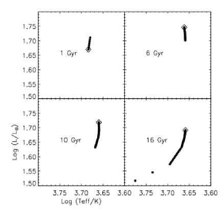
We have used the sample of stars from the Hipparcos catalog described in Kotoneva et al. (2002) and for which accurate metallicities have been derived either from spectroscopy or narrow band photometry. The sample consists of 213 stars with metallicities ranging from [Fe/H] . All stars have accurate photometry and parallax distances from Hipparcos (see Kotoneva et al. (2002)). In Fig. 5 we show the locus of a set of isochrones from our stellar library for different metallicities and ages (at such low luminosities the age makes no difference in the locus of the isochrone). The different symbols correspond to Hipparcos stars from the above mentioned catalog and with the appropriate metallicity. Both solar and sub-solar models provide a good fit to the data, while the super solar model is not so good at higher luminosities but provides a fair fit to the data for . Kotoneva et al. (2002) discuss how other independent sets of isochrones fit the data and conclude that our isochrones are among the best fit to the Hipparcos data. Despite this, attention should be paid to super-solar models since they seem to be difficult to construct.
Having demonstrated that the isochrones provide a good fit to dwarfs of different metallicities we explore how successful they are at fitting the giant branches. Since the age does play a role in the temperature of the giant branch, the test with Hipparcos local stars is not possible. In order to attempt this test we are therefore forced to use star clusters which have much more uncertain distances (and therefore less certain ages as well) than Hipparcos nearby stars but have a simpler star formation history: they are single bursts. However the colour of the giant branches is well determined and therefore provides a good test for the models, specially at low temperatures. So we do adopt distances published in the literature for these cluster and fit the best isochrone to the overall color-magnitude diagram.
In Fig. 6 we show fits to the color-magnitude diagram of several globular and open clusters. In all cases the isochrones provide good fits to the overall shape of the color-magnitude diagram. Further, both the red giant branches and main sequence turn off are well fitted by the isochrones. The fit is good for different colours: the red giant branch of M67 is well fitted for and as well. The fit to the globular cluster 47 Tuc has been done for an age of 11 Gyr and . For M76 we used and an age of 5 Gyr. Finally, NGC188 has been fitted with an isochrone with and 6 Gyr.
We conclude that the stellar interior models provide good fits to available photometry of single stellar populations and individual stars. We are most encouraged by the good fit the isochrones provide to Hipparcos dwarfs since these are the only stars with accurate distances, and therefore absolute magnitude, and metallicities and their color magnitude diagram does not depend on the age of the star. It is also reassuring that the colours of theoretical red giant branches are able to reproduce those of observed clusters.

3 The library of synthetic stellar population spectra


We define a stellar population as a collection of stars formed at a certain rate in a certain chemical environment and whose integrated light we are able to measure. We define a single stellar population (SSP) as a stellar population formed in a uniform chemical environment during a burst of infinitesimal duration (delta function). The steps involved in building a SSP are:
-
1.
A set of stellar tracks of different masses and of the metallicity of the SSP is selected from our library.
-
2.
An isochrone is built for the corresponding age. Each point in the isochrone has a luminosity, effective temperature and gravity that are used to assign the corresponding photospheric model.
-
3.
The fluxes of all stars are summed up, with weights proportional to the stellar initial mass function (IMF).
SSPs are the building blocks of any arbitrarily complicated population since the latter can be computed as a sum of SSPs, once the star formation rate is provided. In other words, the luminosity of a stellar population of age (since the beginning of star formation) can be written as:
| (4) |
where the luminosity of the SSP is:
| (5) |
and is the luminosity of a star of mass , metallicity and age , and are the initial and final metallicities, and are the smallest and largest stellar mass in the population and is the star formation rate at the time when the is formed. In this paper we concentrate in building SSPs, while in previous papers we discuss stellar populations that are consistent with chemical evolution (Jimenez et al., 1998, 2000).
We have computed a large number of SSPs, with ages between and years, and metallicities from to , that is from 0.01 to 5. Fig. 7 shows a set of synthetic spectra of SSPs for three metallicities and ages between and years (from top to bottom).
4 Parameter degeneracies: age and metallicity
SSP are simple, given an IMF, they only depend on two parameters: age and metallicity. It is therefore customary to ask the question: can one recover these two parameters from an observed spectrum? Of course, no single galaxy in the universe is a SSP, since its star formation history is not going to be a single burst, nor its metallicity a single one. However, most (if not all) elliptical galaxies have formed their stellar populations at high redshifts in a very short duration of time (e.g., Jimenez et al. (1999)) and they have relatively uniform chemical compositions, thus their spectra can be correctly described by a SSP.
The so called age-metallicity degeneracy has been the focus of much attention during the past few years (e.g. Wilcots (1994)). Several authors have argued that broad-band colors are degenerate and therefore cannot be used to determine simultaneously age and metallicity of a SSP. Wilcots (1994) has pointed out that certain absorption features can be used to better determine age and metallicity simultaneously. These feature are usually confined to a relatively narrow spectral range ( Å).
In principle there is no need to discard information across the spectrum since all of it may contain information that yields a joint determination of the two parameters. Here we show how the whole spectrum contains information about both age and metallicity and that inclusion of light bluewards of Å helps to break any degeneracy in the age-metallicity plane.
We first select a spectrum from the grid for a given age and metallicity and add random noise. We then try to recover the age and metallicity using minimization, marginalizing over the amplitude. In the first case we limit the spectral range from to Å and add random noise with per resolution element ( Å). We do this for four ages (1, 4, 8 and 12 Gyr) and solar metallicity. The corresponding contour plots of the likelihood surfaces for 1,2 and 3 levels are shown in fig. 8. Already, it can be seen that age and metallicity are not completely degenerate since the contours do close, however the joint determination of age and metallicity is accurate only at the 20% level. This also shows that one does not need to concentrate in special spectral features chosen empirically, the entire spectrum (despite the limited spectral range considered) does contain information.
The above mild degeneracy is completely removed if we add 2000 Å of bluer spectral light. Fig. 9 shows similar plots as the previous figure, but in this case the spectral range of the spectrum goes from to Å similar to that of the SDSS survey. The figure shows that in this case age and metallicity can be recovered with accuracy better than 1% (despite the moderate (10) of the mock test spectra).
Dunlop et al. (2003) reach similar conclusions using real spectra. They find that addition of the same amount of UV light is sufficient to completely determine the age-metallicity and star formation history of an elliptical galaxy.
| Jimenez (true age/Gyr) | 1 | 4 | 8 | 12 |
|---|---|---|---|---|
| BC (recovered age/Gyr) | 1.2 | 3.5 | 7 | 11.1 |
| 0.5 Gyr | ||||
|---|---|---|---|---|
| N-AGB | -0.10 | -0.08 | -0.10 | -0.25 |
| R-AGB | +0.10 | +0.08 | +0.12 | +0.30 |
| N-HB | -0.01 | -0.05 | -0.10 | -0.20 |
| B-HB | -0.05 | -0.02 | -0.05 | -0.05 |
| R-HB | +0.05 | +0.02 | +0.05 | +0.04 |
| 5 Gyr | ||||
| N-AGB | 0.00 | 0.00 | -0.05 | -0.10 |
| R-AGB | 0.00 | 0.00 | +0.05 | +0.20 |
| N-HB | +0.01 | 0.00 | -0.04 | -0.20 |
| B-HB | -0.03 | -0.02 | -0.03 | -0.05 |
| R-HB | 0.00 | 0.00 | +0.03 | +0.03 |
| 14 Gyr | ||||
| N-AGB | +0.01 | +0.01 | +0.01 | -0.08 |
| R-AGB | +0.05 | +0.03 | +0.10 | +0.20 |
| N-HB | -0.10 | -0.04 | +0.04 | +0.10 |
| B-HB | -0.15 | -0.05 | -0.05 | -0.2 |
| R-HB | +0.05 | -0.05 | -0.05 | -0.05 |

5 Systematic errors in SSPs
In the previous section we have shown that given moderate and wavelength spectral coverage, the parameters of a SSP can be accurately recovered. What is the impact of systematics in this parameter determination?
To answer this question and also to assess how our models compare to previous work, we have done the following: first we have compared our models to those by Bruzual & Charlot (2000 models; Bruzual & Charlot (1993)) and Worthey (Wilcots, 1994). Fig. 10 shows the spectral energy distributions as a function of wavelength for 3 different ages. The 3 models differ among each other over the whole spectral range. The models are more similar at older ages than at ages of 1 Gyr. The typical rms variation between our models and those of BC is of % in intensity. How important is this difference? To address this question we have performed the following test: we pick a spectrum from our models (with a fixed age and metallicity) developed in this paper and add gaussian noise with per resolution element of 20 Å. We then attempt to recover the age using Bruzual & Charlot models. Results are presented in Table 2. As can be seen the systematic error in the absolute age is about 10% while the relative age difference is only of a %. We therefore conclude that although systematic differences remain between different models, their impact on parameter recovery is at the same level as the difference in the intensity of the models.
We can also investigate the impact that mass loss can have in, for example, the colours of integrated single stellar populations. In Table 3 we show the change in the integrated colours that different prescritions for mass loss, which translates mostly in the morphology of the HB and termination of the AGB, produce. The impact can be significant in the colors if mass loss is ignored (as much as magnitudes in the infrared), thus careful attention must be payed to this source of systematics.
6 SSP at ultra-high redshift: Primordial Proto–Galaxies
At , traditional optical bands () fall below the rest frame wavelength that corresponds to the Lyman break spectral feature (1216 Å), where most of the stellar radiation is extinguished either by interstellar or intergalactic hydrogen. Because of this, galaxies at are practically invisible at those photometric bands, and even if they were detected, their colors would provide very little information about their stellar population. New detectors and space telescopes, such as SIRTF (http://sirtf.caltech.edu) , and in particular the JWST (http://www.stsci.edu/jwst), will offer the possibility of detecting very distant galaxies at IR wavelengths, and of using photometric redshifts also with far–IR colors, as proposed by Simpson & Eisenhardt (1999); Panagia et al. (2002).
Nearby star forming galaxies are known to contain a considerable amount of dust, that extinguishes a large fraction of their stellar UV light and boosts, even by orders of magnitude, their IR luminosity. The effect of dust must be taken into account in the computation of colors involving photometric bands that span a large wavelength interval. However, the search for very young proto–galaxies, perhaps the first significant star forming systems in the Universe, might be pursued without having to model the effects of dust. The first stars to form in proto–galaxies must have primordial chemical composition, or at least very low metallicity (e.g. Tegmark et al. (1997); Padoan et al. (1997)). Although it is difficult to model the formation and disruption of dust grains on a galactic scale, it is likely that the dust content of a galaxy grows together with its metallicity, and that a proto–galaxy with primordial chemical composition or very low metallicity () has practically no dust (e.g. Jimenez et al. (1999)). In this work we refer to young protogalaxies with metallicity as primordial protogalaxies, or PPGs. We show that, because of their very blue colour, PPGs do not suffer from very strong cosmological dimming, a feature which should aid their detectability in deep infrared surveys with the JWST.
6.1 Spectral energy distribution and IR colors of PPGs

We have computed the SED of PPGs using the extensive set of synthetic stellar population models developed in this paper. In particular, PPGs are modelled using a constant star formation rate and metallicity. As noted above, we expect (and therefore assume) that no photometrically significant quantity of dust has already been formed in PPGs. We also assume that PPGs are young objects (age less or equal than 100 million years). Furthermore, and in order to test the shape of the primordial IMF, we have adopted a Salpeter IMF () with four different low mass cutoff values: 0.1, 2, 5 and 10 M⊙ (i.e. the IMF does not contain any stars with masses below the cut-off values).
The effect of the different low mass cutoff values on the SED of a PPG is shown in fig. 11, where the flux density Fν is plotted in arbitrary units for a 10 million year old PPG with and constant star formation (solid lines). Different solid lines corresponds to the different IMF cutoffs, 0.1, 2, 5 and 10 M⊙, from top to bottom (the 5 and 10 M⊙ are almost overlapped). As expected, the lack of low mass stars translates into a deficit of flux at IR wavelengths. Furthermore, for a low mass cutoff larger than 5 M⊙ the SEDs do not differ much since stars with masses larger than 5 M⊙ have similar spectral energy distributions in the IR. The difference in relative flux density over the wide wavelength range illustrated in fig. 11 provides the means to test the IMF in PPGs. The SED of an observed nearby starburst, from Schmitt et al. (1997), is also plotted in fig. 11 (dashed line), together with a 10 million year model starburst, with continuous star formation, metallicity , and no dust extinction or emission (dotted line). The difference in the spectral slope between PPGs and nearby starbursts is striking, and it is still significant between PPGs and the idealized starburst model with no dust. Although the idealized starburst model with no dust is unlikely to describe any galaxy observed nearby, it can be used as an approximate model for the UV SED of quasars, due to its rather flat SED in the far ultra violet wavelengths.
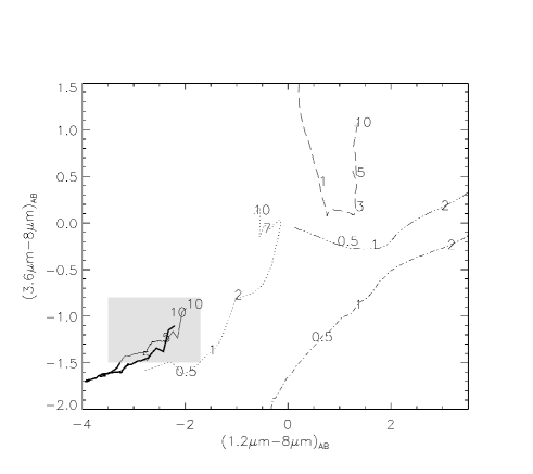
We have computed AB magnitudes (, where is expressed in erg s-1 Hz-1) for 3 different wavelengths: 1.2, 3.6 and 8 m. Fig. 12 shows the colour–colour trajectory for PPGs with a Salpeter IMF with a low mass cutoff of 0.1 M⊙ (thin solid line), and 5 M⊙ (thick solid line), metallicity , and an age of 10 million years. The dashed line is the evolution of the nearby starburst from fig. 12, and the dotted line the evolution of the idealized starburst model with no dust and , also from fig. 12. All models have been simply K–corrected and the numbers that label the trajectories indicate the corresponding redshift. The figure shows that PPGs with redshift range have colors in the range of values mm and mm, that are inside the grey area. The idealized starburst model with no dust and sub–solar metallicity enters marginally the dashed area, but only for low redshifts (). This idealized model is unlikely to describe nearby galaxies, while it can be a rough description of the UV SED of quasars, in which case it could be concluded that PPGs should have very different colors than quasars at redshift (at least about 0.5 mag away in the color–color plot of fig. 12). Nearby galaxies are either star forming galaxies with significant amount of dust (irregular, spiral or starburst galaxies), or older stellar systems with little gas or dust (elliptical galaxies). In both cases nearby galaxies are much redder than PPGs. In fig. 12, the dashed dotted lines show the color–color redshift evolution of two typical nearby galaxies (a spiral and an elliptical galaxies, from Schmitt et al. (1997)). These galaxies, even if nearby, are always at least 2 mag redder than PPGs in the mm color.
The fact that PPGs are the bluest objects, in this IR color–color plot, is an important result, since a photometric search for high redshift galaxies would, in principle, be biased toward selecting the solar metallicity starbursts, which are the reddest galaxies, as already proposed by Simpson & Eisenhardt (1999). Although it cannot be excluded that galaxies of metallicity close to the solar value might exist at , and that PPGs are rare (since they are young by definition), fig. 12 shows that primordial star formation at high redshift should be searched for in very blue objects. The shaded area in fig. 12 marks the expected location of PPGs.
7 The IR Flux Density of PPGs
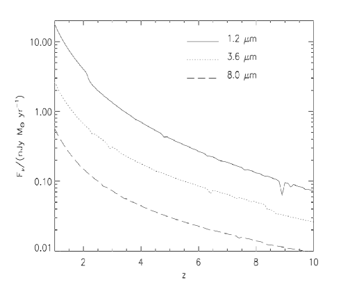
We have just shown that PPGs can be photometrically selected as the bluest galaxies in the Universe. The question that needs to be answered now is: Can PPGs be detected at all with future telescopes such as the SIRTF and the JWST? PPGs could in fact be very faint because they could be very small, or because their star formation rate (SFR) could be very low. To answer this question, we have computed the expected flux in nJy per unit of SFR (in Myr), as a function of redshift, for a PPG with a Salpeter IMF and cutoff mass of 5 M⊙, in a dominated Universe (, , km s-1 Mpc-1). The plots are roughly independent of the starburst age, for age larger than a few million years. Fig. 13 shows that, although PPGs do not exhibit a negative K-correction as galaxies do in sub-mm and mm bands, they suffer from very little cosmological dimming, even in an open Universe. From fig. 13, it can be seen that PPGs with SFR of about Myr have a flux in the faintest band (m) of about 1 nJy (although they would be much brighter at 1.2 m – about 10-20 nJy). The IRAC camera at SIRTF will be able to measure in 1 hour exposure a flux of 500nJy at the 5 level, and will not be able to detect PPGs which a SFR of less than 100 yr-1 but much higher. On the other hand, the JWST time calculator (htpp:/www.stsci.edu/jwst) gives (for a point source using the MIR-ACCUM instrument with a resolution of 3, S/N=5) that exposing 300 hours one can get a flux of about 5nJy at 8m. In order to distinguish PPGs we also need observations at 3.6 and 1.2 m (see fig. 12). using the same calculator we obtain (this time NIR-ACCUM, resolution 3, S/N=5) that it takes 3.63 hours to achieve 1 nJy at 3.6 m, while it takes 3.12 hours at 1.2 m. It is worth noting though that PPGs are expected to be about 1 order of magnitude brighter at 1.2 and 3.6 than at 8 m. Therefore, for the 4 nJy constraint imposed by the 8 m band one would need only a few minutes to achieve the required sensitivity at 1.2 and 3.6 m. It is therefore accurate to say that the limit on our observations comes from the 8 m band solely. Now, inspection of fig. 13 shows that a flux of 5nJy at 8m is achieved for PPGs with SFRs of about 400 M⊙ yr-1. For example, one needs to have systems with ages of 107 yr and masses of a few M⊙ in order for them to achieve a flux of 4nJy. This is not an unreasonable mass for the first objects since it is likely that star formation of the first objects will be retarded until a relatively large halo is in place (Oh & Haiman, 2003).
7.1 The Primordial Stellar IMF
Observational and theoretical arguments suggest that stars forming from gas of very low metallicity () could have an initial mass function (IMF) shifted toward much larger masses than stars formed later on from chemically enriched gas. The observational arguments are extensively discussed in a paper by Larson (1998), and we refer the reader to that work. The main theoretical reason in favor of a ‘massive’ zero metallicity IMF is the relatively high temperature ( K) of gas of primordial composition, that is cooled at the lowest temperatures mainly by H2 molecules (Palla et al., 1983; Mac Low & Shull, 1986; Shapiro & Kang, 1987; Kang et al., 1990; Kang & Shapiro, 1992; Anninos & Norman, 1996). One of the most exciting aspects of the photometric discovery of PPGs would be the possibility of investigating the nature of their stellar IMF, once their redshifts are available.
It is likely that while the local properties of the ISM do not interfere significantly with the self similar dynamics that originate the stellar IMF, they do play a role in setting the particular value of the mass scale where the self similarity is broken. According to this point of view, one expects the stellar IMF to have always more or less the same power law shape, down to a cutoff mass whose value depends on local properties of the ISM, and up to the largest stellar mass, whose value is limited either by the total mass of the star formation site, or by some physical process that prevents the formation of super–massive stars.
The lower mass cutoff of the stellar IMF has been predicted in models of i) opacity limited gravitational fragmentation (Silk, 1977a, b, c; Yoshii & Saio, 1985, 1986); ii) protostellar winds that would stop the mass accretion onto the proto-star (Adams & Fatuzzo, 1996); iii) fractal mass distribution with fragmentation down to one Jeans’ mass (Larson, 1992). If gravitational sub–fragmentation during collapse is not very efficient (see Boss (1993)), the value of the Jeans’ mass determines the lower mass cutoff of the IMF. In Padoan et al. (1997), numerical simulations of super–sonic and super–Alfvénic (Padoan & Nordlund, 1999) magneto–hydrodynamic turbulence are used to compute the probability density function of the gas density, which is used to predict the distribution of the Jeans’ mass in turbulent gas, under the reasonable assumption of uniform kinetic temperature. The Jeans’ mass distribution computed in Padoan et al. (1997) has an exponential cutoff below a certain mass value, that is found to be:
| (6) |
where is the gas temperature, the gas density, and the gas velocity dispersion. Using the ISM scaling laws, according to which , one obtains:
| (7) |
that is a few times smaller that the average Jeans mass (the Jeans mass corresponding to the average gas density), and therefore an important correction to more simple models of gravitational fragmentation, that do not take into account the effect of super–sonic turbulence on the gas density distribution.
If the ISM has primordial chemical composition, and the main coolant is molecular hydrogen, a temperature below K is hardly reached, and the stellar IMF might have a lower mass cutoff of about M⊙. Similar lower mass cutoffs are obtained in the models by Silk (1977c) and Yoshii & Saio (1986), who estimated typical stellar masses, based on molecular hydrogen cooling, of approximately and M⊙ respectively. More recent numerical simulations of the collapse and cooling of cosmological density fluctuations of large amplitude (the first objects to collapse in the Universe), yield even larger values of the Jeans’ mass, of the order of M⊙ (Bromm, Coppi, & Larson 1999; Abel, Bryan, & Norman 1998)
The discovery of PPGs could shed new light on the problem of the primordial IMF. The redshift evolution of the two colors mm and mm, computed with the PPG model discussed in this work, is plotted in fig. 14. The solid line is the case of a PPG with a Salpeter IMF with M⊙ cutoff, and the dashed line the same PPG model, but with a M⊙ cutoff. Once a PPG candidate is selected with the IR broad band photometry as a very blue object (colors inside the shaded area in fig 12), and its redshift is estimated with a Lyman drop method, or with an H search, the IR colours provide a tool to discriminate between a standard IMF, and an IMF deprived of low mass stars. The lower panel of fig 14 shows that a PPG with a ’massive’ IMF can be about 0.5 mag bluer in mm than a PPG with a standard IMF.

7.2 Detectability via broad-band infrared imaging versus emission-line searches
In this work we propose to select PPGs as the bluest objects in deep IR surveys, on the basis of the color–color plot shown in fig. 2. We now address the question of how a broad band photometric selection of PPGs performs, compared with searches of emission lines, such as Lyman- and H. The rest frame equivalent widths of Lyman- and H can be very roughly estimated by assuming that each photon below 1251 and 1025 Å will originate a Lyman- and H photon respectively. The equivalent widths estimated in this way are of course upper limit to the true equivalent widths. We find that the equivalent width of Lyman- is 380 Å while the equivalent width of H is 4400 Å –the latter is so high due to the fact that the continuum at 6563 Å is rather faint in PPGs (see Fig. 11). Assuming that the lines have intrinsic widths at rest–frame typical of the virial velocity of a galaxy (for example a line width of 300 km/s corresponds to 2 and 13 Å respectively), one finds that they will only be about 30 times brighter than the continuum at . Since one would need to shift the narrow filter for about 500 steps, or more, to search for all possible emitters in the redshift range , the advantage of the lines being brighter than the continuum is offset by the number of steps needed to find all PPGs between and 10. It seems therefore that IR broad band photometry is an easier way to both detect and select PPG candidates than the emission line technique, because only one deep exposure is needed to find all PPGs in the redshift range . Note that the equivalent width of Lyman- and H has been over–estimated here. Moreover, the advantage of deep broad band photometry is that, together with detecting and selecting PPGs, it provides at the same time important information about their stellar populations. However, it is important that the emission line technique (or a Lyman break technique) is available aboard the NGST, since photometric redshifts measured with narrow filters will probably be the best (or the only) way to further constrain the redshift of PPG broad band photometric candidates, which is necessary to extract information about their stellar population from the broad band colors (fig. 4)111We note in passing that the acquisition of photometry around the Lyman break to determine their redshift would not be time consuming as shown before and that the biggest limitation in detecting PPGs is due to the poor performance of the 8 m detectors..
A star formation rate of Myr over a few million years is necessary for detecting a PPG with the JWST. With such SFR, after years M⊙ of gas is turned into stars. In order to still have a metallicity of , these stars must be formed in a system with baryonic mass of at least M⊙, that is a very large galaxy, or a small group of galaxies. Such massive systems are inside large dark matter halos that are not collapsing yet at redshift . It is possible that PPGs that can be detected with the JWST are the progenitors of very large galaxies, in a phase when their dark matter halo has not turned around yet. If PPGs are discovered, their spectro–photometric properties could give very important clues for the problem of star formation in galaxies (such as the origin of the stellar IMF) and their luminosity, abundance, and redshift distribution would trace the complete history of the very first star formation sites in the Universe.
8 Conclusions
In this paper we have presented new stellar interior tracks and single stellar population models of arbitrary age, metallicity and IMF. Our main findings are:
-
1.
A new set of stellar interior models has been presented. The models cover all stages of stellar evolution and we have built isochrones out of them for ages between .
-
2.
It is possible to construct stellar evolution models that accurately reproduce the properties of individual stars for a wide range of ages and metallicities.
-
3.
We have presented a new algorithm to compute the evolution of stars in the RGB, HB and AGB. This algorithm makes it possible to explore the effect of variations in some of unknown parameters of stellar evolution like mass loss, mixing length etc.
-
4.
We have developed a new and fast algorithm to build synthetic stellar evolution spectra and colour–magnitude diagrams of arbitrary metallicity and age.
-
5.
We have shown that changes in the values of the stellar parameters like mass loss and mixing length can change the predicted colours of a population by as much as 0.4 mag.
-
6.
We have studied degeneracies in the parameter space (age and metallicity) and shown that these parameters are only degenerated if the wavelength range of the spectrum is very small or only a few spectral features are chosen. Addition of light bluewards of the Å ( Å) significantly reduces this degeneracies and, in fact, lifts them.
-
7.
It has been shown that systematic errors among different models are at the level of 10-20%, despite using completely different stellar input physics. It should be possible to reduce these errors even further.
-
8.
We have studied the photometric properties of very young proto–galaxies with primordial or very low () metallicity and no significant effect of dust in their SED. We have named these galaxies “primordial protogalaxies”, or PPGs. Using the methods of synthetic stellar populations, we predict that PPGs are the bluest stellar systems in the Universe. They can therefore be selected in color–color diagrams obtained with deep broad band IR surveys, and can be detected with the JWST, if they have a SFR of at least Myr, over a few million years. We have discussed the possibility of using the IR colours of PPGs to constrain their stellar IMF, and investigated the possibility that the stellar IMF arising from gas of primordial chemical composition is more “massive” than the standard Salpeter IMF. Finally we have argued that broad band photometry can be more efficient than emission line searches, to detect and select PPGs.
The models are available on the world wide web (www.roe.ac.uk/jsd and www.physics.upenn.edu/raulj). We provide the stellar interior tracks presented in this paper and the single stellar population models and tools to compute photometry and synthetic stellar populations with arbitrary star formation histories.
acknowledgments
We thank the referee, Guy Worthey, for comments that greatly improved this paper. RJ thanks Eric Agol and Marc Kamionkowski for encouraging him to publish the stellar models contained in this paper. The work of RJ is partially supported by NSF grant AST-0206031. James Dunlop acknowledges the enhanced research time provided by the award of a PPARC Senior Fellowship.
References
- Abbott (1982) Abbott D. C., 1982, ApJ, 263, 723
- Adams & Fatuzzo (1996) Adams F. C., Fatuzzo M., 1996, ApJ, 464, 256
- Alexander & Ferguson (1994) Alexander D., Ferguson J., 1994, ApJ, p. 879
- Angulo et al. (1999) Angulo et al. 1999, Nuclear Physics A, 656, 3
- Anninos & Norman (1996) Anninos P., Norman M. L., 1996, ApJ, 460, 556
- Arimoto & Yoshii (1987) Arimoto N., Yoshii Y., 1987, A&A, 173, 23
- Barbaro & Bertelli (1977) Barbaro C., Bertelli C., 1977, A&A, 54, 243
- Barbaro & Olivi (1986) Barbaro G., Olivi F. M., 1986, in Spectral Evolution of Galaxies Spectrophotometric models of galaxies. pp 283–306
- Beaudet et al. (1967) Beaudet G., Petrosian V., Salpeter E. E., 1967, ApJ, 150, 979
- Bessell (1998) Bessell M. S., 1998, in IAU Symp. 189: Fundamental Stellar Properties Cool star empirical temperature scales. p. 127
- Boss (1993) Boss A. P., 1993, ApJ, 410, 157
- Bressan et al. (1994) Bressan A., Chiosi C., Fagotto F., 1994, ApJ, 94, 63
- Bruzual (1983) Bruzual G. A., 1983, ApJ, 273, 105
- Bruzual & Charlot (1993) Bruzual G. A., Charlot S., 1993, ApJ, 405, 538
- Chaboyer (1995) Chaboyer B., 1995, ApJL, 444, L9
- Chaboyer & Krauss (2002) Chaboyer B., Krauss L. M., 2002, ApJL, 567, L45
- Charlot & Bruzual (1991) Charlot S., Bruzual A. G., 1991, ApJ, 367, 126
- Charlot et al. (1996) Charlot S., Worthey G., Bressan A., 1996, ApJ, 457, 625
- Dunlop et al. (2003) Dunlop J., Nolan L., Jimenez R., Heavens A., 2003, astro-ph/03xxxxx
- Dunlop et al. (1996) Dunlop J., Peacock J., Spinrad H., Dey A., Jimenez R., Stern D., Windhorst R., 1996, Nature, 381, 581
- Eggleton (1971) Eggleton P. P., 1971, MNRAS, 151, 351
- Eggleton (1972) Eggleton P. P., 1972, MNRAS, 156, 361
- Eggleton et al. (1973) Eggleton P. P., Faulkner J., Flannery B. P., 1973, A&A, 23, 325
- Fioc & Rocca-Volmerange (1997) Fioc M., Rocca-Volmerange B., 1997, A&A, 326, 950
- Fontaine et al. (1977) Fontaine G., Graboske H. C., van Horn H. M., 1977, ApJS, 35, 293
- Guiderdoni & Rocca-Volmerange (1987) Guiderdoni B., Rocca-Volmerange B., 1987, A&A, 186, 1
- Haft et al. (1994) Haft M., Raffelt G., Weiss A., 1994, ApJ, 425, 222
- Heavens & Jimenez (1999) Heavens A. F., Jimenez R., 1999, MNRAS, 305, 770
- Iben & MacDonald (1995) Iben I., MacDonald J., 1995, in LNP Vol. 443: White Dwarfs Vol. , The Born Again AGB Phenomenon. p. 48
- Iben et al. (1992) Iben I. J., Fujimoto M. Y., MacDonald J., 1992, ApJ, 388, 521
- Iglesias & Rogers (1996) Iglesias C. A., Rogers F. J., 1996, ApJ, 464, 943
- Itoh et al. (1979) Itoh N., Totsuji H., Ichimaru S., Dewitt H. E., 1979, ApJ, 234, 1079
- Jimenez et al. (1998) Jimenez R., Flynn C., Kotoneva E., 1998, MNRAS, 299, 515
- Jimenez et al. (2003) Jimenez R., Flynn C., MacDonald J., Gibson B. K., 2003, Science, in press
- Jimenez et al. (1999) Jimenez R., Friaca A. C. S., Dunlop J. S., Terlevich R. J., Peacock J. A., Nolan L. A., 1999, MNRAS, 305, L16
- Jimenez et al. (1995) Jimenez R., Jorgensen U. G., Thejll P., Macdonald J., 1995, MNRAS, 275, 1245
- Jimenez et al. (2000) Jimenez R., Padoan P., Dunlop J. S., Bowen D. V., Juvela M., Matteucci F., 2000, ApJ, 532, 152
- Jimenez et al. (1998) Jimenez R., Padoan P., Matteucci F., Heavens A. F., 1998, MNRAS, 299, 123
- Jimenez et al. (1996) Jimenez R., Thejll P., Jorgensen U. G., Macdonald J., Pagel B., 1996, MNRAS, 282, 926
- Jimenez et al. (1999) Jimenez et al. 1999, astro-ph, 9910279
- Jorgensen (1991) Jorgensen U. G., 1991, A&A, 246, 118
- Jorgensen & Jimenez (1997) Jorgensen U. G., Jimenez R., 1997, A&A, 317, 54
- Jorgensen & Thejll (1993) Jorgensen U. G., Thejll P., 1993, A&A, 272, 255
- Kang & Shapiro (1992) Kang H., Shapiro P. R., 1992, ApJ, 386, 432
- Kang et al. (1990) Kang H., Shapiro P. R., Fall S. M., Rees M. J., 1990, ApJ, 363, 488
- Knapp et al. (1998) Knapp G. R., Young K., Lee E., Jorissen A., 1998, ApJS, 117, 209
- Kotoneva et al. (2002) Kotoneva E., Flynn C., Jimenez R., 2002, MNRAS, 335, 1147
- Larson (1992) Larson R. B., 1992, MNRAS, 256, 641
- Larson (1998) Larson R. B., 1998, MNRAS, 301, 569
- Lee et al. (2002) Lee H., Lee Y., Gibson B. K., 2002, AJ, 124, 2664
- Mac Low & Shull (1986) Mac Low M. M., Shull J. M., 1986, ApJ, 302, 585
- Mihalas (1978) Mihalas D., 1978, in Stellar atmospheres, San Francisco: W.H. Freeman, 1978 Stellar atmospheres
- Nolan et al. (2003) Nolan L., Dunlop J., Jimenez R., Heavens A. F., 2003, MNRAS, 341, 464
- Nolan et al. (2001) Nolan L. A., Dunlop J. S., Jimenez R., 2001, MNRAS, 323, 385
- Oh & Haiman (2003) Oh S., Haiman Z., 2003, astro-ph/0307135
- Padoan et al. (1997) Padoan P., Jimenez R., Antonuccio-Delogu V., 1997, ApJ, 481, 27L
- Padoan et al. (1997) Padoan P., Jimenez R., Jones B. J. T., 1997, MNRAS, 285, 711
- Padoan & Nordlund (1999) Padoan P., Nordlund Å., 1999, ApJ, 526, 279
- Padoan et al. (1997) Padoan P., Nordlund Å., Jones B., 1997, ApJ, 474, 730
- Palla et al. (1983) Palla F., Salpeter E. E., Stahler S. W., 1983, ApJ, 271, 632
- Panagia et al. (2002) Panagia N., Stiavelli M., Ferguson H. C., Stockman H. S., 2002, in Galaxy evolution, theory and observations Primordial Stellar Populations
- Ramadurai (1976) Ramadurai S., 1976, MNRAS, 176, 9
- Reimers (1975) Reimers D., 1975, Circumstellar envelopes and mass loss of red giant stars. Problems in Stellar Atmospheres and Envelopes, pp 229–256
- Renzini (1981) Renzini A., 1981, in Colors and Populations of Galaxies - Paris Energetics of stellar populations. p. 87
- Renzini & Buzzoni (1983) Renzini A., Buzzoni A., 1983, Memorie Societa Astronomica Italiana, 54, 739
- Salpeter & van Horn (1969) Salpeter E. E., van Horn H. M., 1969, ApJ, 155, 183
- Schaller et al. (1992) Schaller G., Schaerer D., Meynet G., Maeder A., 1992, A&AS, 96, 269
- Schmitt et al. (1997) Schmitt H. R., Kinney A. L., Calzetti D., Storchi Bergmann T., 1997, AJ, 114, 592
- Shapiro & Kang (1987) Shapiro P. R., Kang H., 1987, ApJ, 318, 32
- Silk (1977a) Silk J., 1977a, ApJ, 211, 638
- Silk (1977b) Silk J., 1977b, ApJ, 214, 152
- Silk (1977c) Silk J., 1977c, ApJ, 214, 718
- Simpson & Eisenhardt (1999) Simpson C., Eisenhardt P., 1999, PASP, 111, 691
- Spinrad et al. (1997) Spinrad H., Dey A., Stern D., Dunlop J., Peacock J., Jimenez R., Windhorst R., 1997, ApJ, 484, 581
- Stringfellow et al. (1990) Stringfellow G. S., Dewitt H. E., Slattery W. L., 1990, Phys. Rev. A, 41, 1105
- Tegmark et al. (1997) Tegmark M., Silk J., Rees M. J., Blanchard A., Abel T., Palla F., 1997, ApJ, 474, 1
- Tinsley (1968) Tinsley B. M., 1968, ApJ, 151, 547
- Werley et al. (1984) Werley M., Norman M., Newman 1984, J. Phys. D, 12, 408
- Wilcots (1994) Wilcots E. M., 1994, AJ, 107, 1338
- Worthey (1994) Worthey G., 1994, ApJ Suppl., 95, 107
- Yoshii & Saio (1985) Yoshii Y., Saio H., 1985, ApJ, 295, 521
- Yoshii & Saio (1986) Yoshii Y., Saio H., 1986, ApJ, 301, 587
9 Appendix: Analytic fits for colours of SSPs
The magnitudes for a SSP (normalized to 1 M⊙) as a function of age and metallicity, for a given photometric band UBVRIJK, are approximated to within 4% by:
| (8) |
where
| (9) | |||||
| (10) | |||||
and
| (11) |
Luminosities are obtained simply from , where for . The and values appear as exponents of and , respectively, and as indexes defining elements of the matrices, given by
| (12) |
| (13) |
| (14) |
| (15) |
| (16) |
| (17) |
| (18) |