What is the SUSY mass scale?

Abstract

The energy, or mass scale $M_{\rm SUSY}$, of the supersymmetry (SUSY) phase transition is, as yet, unknown. If it is very high (i.e., $\gg 10^{3}\,{\rm GeV}$), terrestrial accelerators will not be able to measure it. We determine $M_{\rm SUSY}$ here by combining theory with the cosmic microwave background (CMB) data. Starobinsky suggested an inflationary cosmological scenario in which inflation is driven by quantum corrections to the vacuum Einstein’s equation. The modified Starobinsky model (MSM) is a natural extension of this. In the MSM, the quantum corrections are the quantum fluctuations of the supersymetric (SUSY) particles, whose particle content creates inflation and whose masses terminate it. Since the MSM is difficult to solve until the end of the inflation period, we assume here that an effective inflaton potential (EIP) that reproduces the time dependence of the cosmological scale factor of the MSM can be used to make predictions for the MSM. We predict the SUSY mass scale to be $M_{\rm SUSY}\simeq 10^{15}{\rm GeV}$, thus satisfying the requirement that the predicted density fluctuations of the MSM be in agreement with the observed CMB data.

Managing Editor

1 Introduction

Cosmological models based on the anomaly-induced effective action of gravity take into account the vacuum quantum effects of particles in the early universe. These models naturally lead to inflation, which is a direct consequence of the assumption that, at high energies, all particles can be described by massless, conformally invariant fields with negligible interaction between them. [1][5]

In the modified version of the original Starobinsky model [2] [modified Starobinsky model (MSM)], it was assumed that some of the scalar and fermion fields are massive. [4][6] If we also assume a supersymmetric particle content, inflation is, then, stable during the period which starts at a sub-Planck scale, continuing almost until the end of inflation, when most of the sparticles decouple. [6][9] Subsequently, the universe enters into an unstable regime, eventually undergoing a transition to the FRW evolution. It is to be noted that this occurs without any need for fine-tuning, regardless of the values of the cosmological constant $\Lambda$ and the curvature parameter $k$.

In fact both the cosmological constant $\Lambda$ and the curvature $k$ are very small in the context of the high-T early universe. Present observations indicate that the curvature $k$-term is less than $10\%$ of the energy density term in the Friedmann equation and that the $\Lambda$ term is comparable to the energy density term in the $\Lambda$CDM model. Extrapolating back to the high-T early universe, the $k$-term is then $\lesssim 10^{-50}\%$ and the $\Lambda$ term $\lesssim 10^{-100}\%$ of the energy density term. The $k$-term is thus not included in our equations and the $\Lambda$-term is included up to Eq.(17), just for completeness. We set $\Lambda=0$ in the equations after Eq.(17).

It is not possible to solve analytically the equation for the cosmological scale factor $a(t)$ in the MSM. However an approximate solution for $a(t)$ during inflation was obtained and confirmed by numerical analysis with very high precision. [6]

We assume here that an effective inflaton potential (EIP) that reproduces the time dependence of $a(t)$ of the MSM during the inflationary period can be used to make predictions of the MSM throughout this period, including its end. We use a reverse engineering method, discussed in Ref. ellis1, to derive the EIP from $a(t)$.

In $\S$ 2, we give a brief review of anomaly-induced inflation of the MSM and the approximate time dependence of $a(t)$. The effective potential and value for $M_{\rm SUSY}$ are derived in $\S$ 3. Our conclusions are presented in $\S$ 4.

2 The approximate solution of the cosmological scale factor in the modified Starobinsky model

The interesting property of the Starobinsky model is that inflation is a result of vacuum quantum effects of predicted (e.g., SUSY) particles. In the simplest case, based on the effects of massless fields, the leading quantum phenomenon is the conformal anomaly. The underlying theory includes $N_{0}$ scalars, $N_{1/2}$ Dirac spinors, and $N_{1}$ vectors, corresponding to the particle content of the quantum theory. They are not necessarily the real matter filling the universe, whose energy density is assumed to be negligible during inflation. The vacuum quantum effects originate from the virtual particles.

Due to conformal invariance, the fields decouple from the conformal factor of the metric. In this case, the dominating quantum effect is the trace anomaly, which comes from the renormalization of the conformal invariant part of the vacuum action, [11, 12]

$$S_{vacuum}\,=\,S_{HD}\,+\,S_{EH}\,,$$ (1)

where the first term contains higher derivatives of the metric,

$$S_{HD}\,=\,\int d^{4}x\sqrt{-g}\,\left\{a_{1}C^{2}+a_{2}E+a_{3}{\nabla^{2}}R\right\}\,,$$ (2)

and

$$S_{EH}\,=\,-\,\frac{1}{16\pi G}\,\int d^{4}x\sqrt{-g}\,(R+2\Lambda)\,$$

is the Einstein-Hilbert term, where $\,a_{1,2,3},\,G,\,$ and $\,\Lambda\,$ are the parameters of the vacuum action. $C^{2}$ and $E$ are the square of the Weyl tensor and the integrand of the Gauss-Bonnet term, respectively:

$$C^{2}=R_{\mu\nu\alpha\beta}^{2}-2R_{\alpha\beta}^{2}+1/3\,R^{2}\,,$$

$$E=R_{\mu\nu\alpha\beta}R^{\mu\nu\alpha\beta}-4\,R_{\alpha\beta}R^{\alpha\beta}+R^{2}\,.$$

Quantum corrections to the Einstein equation,

$$R_{\mu\nu}\,-\,\frac{1}{2}\,R\,g_{\mu\nu}\,=\,8\pi G\,<T_{\mu\nu}>\,-\,\Lambda\,,$$

produce a non-trivial effect due to the anomalous trace of the energy-momentum tensor. The anomaly-induced effective action can be found explicitly. [12][14] The expression for the anomalous energy-momentum tensor is

$$T\,\,=\,\,<T_{\mu}^{\mu}>\,\,=\,\,-\frac{2}{\sqrt{-g}}\,g_{\mu\nu}\frac{\delta{\Gamma}}{\delta g_{\mu\nu}}\,\,=\,\,-\,(wC^{2}+bE+c{\nabla^{2}}R)\,,$$ (3)

where $w,\,b$ and $c$ are the $\beta$-functions for the parameters $a_{1},\,a_{2},\,a_{3}$ in Eq.(2), respectively:

$$w\,=\,\frac{1}{(4\pi)^{2}}\,\Big{(}\frac{N_{0}}{120}+\frac{N_{1/2}}{20}+\frac{N_{1}}{10}\Big{)}\,,$$ (4)

$$b\,=\,-\,\frac{1}{(4\pi)^{2}}\,\Big{(}\frac{N_{0}}{360}+\frac{11\,N_{1/2}}{360}+\frac{31\,N_{1}}{180}\Big{)}\,,$$ (5)

$$c\,=\,\frac{1}{(4\pi)^{2}}\,\Big{(}\frac{N_{0}}{180}+\frac{N_{1/2}}{30}-\frac{N_{1}}{10}\Big{)}\,$$ (6)

and $\Gamma$ is the quantum correction to the classical vacuum action, taking into account the vacuum quantum effects of the matter fields, which are free, massless, and conformally coupled to the metric. In terms of the new variables, $\bar{g}_{\mu\nu}$ and $\sigma\,(=\ln a(t))$, where $a(t)$ is the cosmic scale factor and $g_{\mu\nu}=\bar{g}_{\mu\nu}\,.\,e^{2\sigma}$, the quantum correction to the classical vacuum action is

$${\bar{\Gamma}}=S_{c}[{\bar{g}}_{\mu\nu}]+\int d^{4}x\sqrt{-{\bar{g}}}\,\{w\sigma{\bar{C}}^{2}+b\sigma({\bar{E}}-\frac{2}{3}{\bar{\Box}}{\bar{R}})+2b\sigma{\bar{\Delta}}\sigma\,\}$$

$$-\frac{3c+2b}{36}\,\int d^{4}x\sqrt{-g}\,R^{2}\,,$$ (7)

where $\,S_{c}[{\bar{g}}_{\mu\nu}]=S_{c}[g_{\mu\nu}]\,$ is some unknown functional of the metric. In general, there is no standard method for deriving $S_{c}[{\bar{g}}_{\mu\nu}]$. If we consider an isotropic and homogeneous metric, $g_{\mu\nu}={\bar{g}}_{\mu\nu}\cdot a^{2}(\eta)$, where $\eta$ is the conformal time, the conformal functional $S_{c}[{\bar{g}}_{\mu\nu}]$ is constant. In this case, $\,S_{c}[{\bar{g}}_{\mu\nu}]$ does not depend on $a(\eta)$ and, therefore, does not contribute to the equations of motion [Eq.(7)] which is an exact one-loop quantum correction.

The total action with quantum corrections is

$$S_{total}=S_{vacuum}+\Gamma\,,$$ (8)

which leads to the following equation of motion for $a(t)$:

$$\frac{{\stackrel{{\scriptstyle....}}{{a}}}}{a}+3\,\frac{{\stackrel{{\scriptstyle.}}{{a}}}}{a}\frac{{\stackrel{{\scriptstyle...}}{{a}}}}{a}+\frac{{\stackrel{{\scriptstyle..}}{{a}}}^{2}}{a^{2}}-\left(5+\frac{4b}{c}\right)\frac{{\stackrel{{\scriptstyle..}}{{a}}}}{a}\frac{{\stackrel{{\scriptstyle.}}{{a}}}^{2}}{a^{2}}-\frac{M^{2}_{\rm Pl}}{c}\left(\frac{{\stackrel{{\scriptstyle..}}{{a}}}}{a}+\frac{{\stackrel{{\scriptstyle.}}{{a}}}^{2}}{a^{2}}-\frac{2\Lambda}{3}\right)\,=\,0\,,$$ (9)

where $\,M_{\rm Pl}=1/\sqrt{8\pi G}=2.44\times 10^{18}\,{\rm GeV}$ is the reduced Planck mass. The dot over the variable denotes the derivative with respect to the physical time $t$, which is related to the conformal time $\eta$ by the relation $dt=a(\eta)d\eta$.

The last term in Eq.(9) is the trace of the standard classical Einstein equation when equated to $(3p-\rho)/6c$, where $p\,(\rho)$ is the pressure (energy density) of the free particles and $c$ is given by Eq.(6). There are only vacuum fluctuations (virtual particles) in Eq.(9) and no free particles. The other terms (the quantum corrections) become negligible if we assume that we have a FRW evolution at late times with $a(t)\sim t^{2/3}$ in a matter dominated era, by massive particles having negligible pressure, for example. The equation of motion [Eq.(9)] is, then, equal to $-\rho_{M}^{0}/6a^{3}c$, instead of being homogeneous. The quantum correction terms have ${\stackrel{{\scriptstyle....}}{{a}}},\,{\stackrel{{\scriptstyle.}}{{a}}}{\stackrel{{\scriptstyle...}}{{a}}},\,{\stackrel{{\scriptstyle..}}{{a}}}^{2},\,{\stackrel{{\scriptstyle..}}{{a}}}{\stackrel{{\scriptstyle.}}{{a}}}^{2}$, which are proportional to the fourth derivative of time of the cosmic scale factor $a$, while the classical Einstein term is proportional to ${\stackrel{{\scriptstyle..}}{{a}}}$ and ${\stackrel{{\scriptstyle.}}{{a}}}^{2}$, the second derivative of time of $a$. We thus expect that the quantum correction terms will not contribute appreciably when the cosmic scale factor is varying slowly with time (e.g., $a\propto t^{2/3}$ in a matter dominated universe or $a\propto t^{1/2}$ in a radiation dominated universe).

Using the FRW metric with $k=0$, the solution to Eq.(9) is

$$a(t)\,=\,a_{0}\cdot\exp(Ht)\,,$$ (10)

where $H$ has the form

$$H\,=\,\frac{1}{\sqrt{(-32\pi G)b}}\cdot\left(\,1\pm\,\sqrt{1+\frac{(64\pi G)\,b\,\Lambda}{3}\,\,}\right)^{1/2}\,.$$ (11)

We do not consider solutions with negative $H$ or $k=\pm 1$. The general equation of motion for $a(t)$ and solutions with $k=\pm 1$ can be found in Ref. asta. When $\Lambda=0$, the solution Eq.(9) is

$$H\,=\,\frac{1}{\sqrt{(-16\pi G)\,b}}\equiv H_{S}\,,$$ (12)

which is the solution for $a(t)$ in the original Starobinsky model. [2]

The inflationary solution (10) is stable for $c>0$ and unstable for $c<0$, [2] regardless of the cosmological constant. [4] According to Eq.(6), the condition $c>0$ requires

$$N_{1}\,<\,\frac{1}{3}\,N_{1/2}\,+\,\frac{1}{18}\,N_{0}\,.$$ (13)

This enables the construction of an attractive inflationary scenario. [7] The universe could start in a stable phase, such that inflation starts regardless of the initial data. The simplest way to provide stability in Eq.(13) is to assume that supersymmetry exists in the high energy region at the beginning of inflation and that it is broken at a lower energy since the sparticles are heavy and decouple. [6, 7] During inflation, $H$ decreases due to the massive fields and, at some point, the loops of the sparticles decouple and the matter content $N_{0,1/2,1}$ becomes modified. As a result, the inequality sign in Eq.(13) changes and the universe enters into an unstable inflation regime with an eventual transition to the FRW evolution.

The intermediate transition epoch between inflation and post-inflation is characterized by vacuum quantum effects of both massive and massless fields. [6, 8] In this epoch, the conformal invariance of the actions is violated by the masses and, therefore, we cannot use the conformal anomaly to derive quantum corrections. However, the conformal description of the massive theory in the framework of the cosmon model can be used [15][18] (see also Refs. sola89–tomb for similar analyzes and applications of the cosmon method). A detailed discussion of the effects of massive fields, including quantum corrections, can be found in Ref. asta.

A leading-log approximation for the effective action for the massive fields,

$$\Gamma\,\,=\,\,S_{HD}+S_{c}[g_{\mu\nu},M]\,+\,\int d^{4}x\sqrt{-{\bar{g}}}\,\{w{\bar{C}}^{2}\sigma+b({\bar{E}}-\frac{2}{3}{\bar{\nabla}}^{2}{\bar{R}})\sigma+2b\,\sigma{\bar{\Delta}}\sigma\}\,-$$

$$\,-\,\frac{3c+2b}{36}\,\int d^{4}x\sqrt{-g}\,R^{2}\,-\,\int d^{4}x\sqrt{-{\bar{g}}}\,e^{2\sigma}\,[{\bar{R}}+6({\bar{\nabla}}\sigma)^{2}]\,\cdot\,\Big{[}\,\frac{1}{16\pi G}-f\cdot\sigma\,\Big{]}\,-$$

$$-\int d^{4}x\sqrt{-{\bar{g}}}\,e^{4\sigma}\,\cdot\,\Big{[}\frac{\Lambda}{8\pi G}\,-\,g\cdot\sigma\,\Big{]}\,,$$ (14)

holds in the high energy region until a “cut off” scale, defined such that at $H=M_{*}$ is reached, when a number of the sparticles decouple. The inflation then becomes unstable, and enters the FRW phase.

The equation of motion for $\sigma(t)=\ln{a(t)}$ in the flat case $k=0$, has the form

$${\stackrel{{\scriptstyle....}}{{\sigma}}}+7{\stackrel{{\scriptstyle...}}{{\sigma}}}{\stackrel{{\scriptstyle.}}{{\sigma}}}+4\,{{\stackrel{{\scriptstyle..}}{{\sigma}}}}^{2}+4\,\Big{(}3-\,\frac{b}{c}\Big{)}\,{\stackrel{{\scriptstyle..}}{{\sigma}}}{{\stackrel{{\scriptstyle.}}{{\sigma}}}}^{2}-4\,\frac{b}{c}\,{{\stackrel{{\scriptstyle.}}{{\sigma}}}}^{4}\,\,+\,\,\frac{2\,\Lambda}{3}\frac{M^{2}_{\rm Pl}}{c}\,(1-\tilde{g}\sigma-\tilde{g}/4)\,-$$

$$-\,\frac{M^{2}_{\rm Pl}}{c}\,\Big{[}\,({\stackrel{{\scriptstyle..}}{{\sigma}}}\,+2{{\stackrel{{\scriptstyle.}}{{\sigma}}}}^{2})\cdot(1-\tilde{f}\sigma)-\frac{1}{2}\,\tilde{f}\dot{\sigma}^{2}\,\Big{]}\,=\,0\,,$$ (15)

where

$$\tilde{f}=(16\pi G)\,f=\frac{2}{3{(4\pi)}^{2}}\,\sum_{f}\,\frac{N_{f}\,m_{f}^{2}}{M^{2}_{\rm Pl}}\,,$$

$$\tilde{g}=\frac{g}{\Lambda/(8\pi G)}\,\,=\,\frac{1}{2(4\pi)^{2}}\,\sum_{s}\,\frac{N_{s}\,m_{s}^{4}}{M^{2}_{\rm Pl}\Lambda}-\frac{2}{(4\pi)^{2}}\,\sum_{f}\,\frac{N_{f}\,m_{f}^{4}}{M^{2}_{\rm Pl}\Lambda}\,.$$ (16)

In Eq.(16), the sums are taken over all fermions with a mass $m_{f}$ and multiplicity $N_{f}$ as well as over all scalars with a mass $m_{s}$ and multiplicity $N_{s}$. It can be seen that the higher-derivative terms of (14) are identical to those for the massless fields, as expected. [3, 11]

Although the solution of Eq.(15) can not be performed analytically, an approximate solution can be obtained. From Eqs.(10) and (11), $\sigma(t)\left(=\ln a(t)\right)$ is proportional to $t$, for small $t$. However, inflation slows down at larger $t$, when $\sigma(t)$ is no longer linear in $t$ due to the masses of the particles. We then approximate $\sigma(t)$ as a second order term in time, $\sigma(t)=A\times t+B\times t^{2}$, where $A$ and $B$ are constants and $B$ is negative. The equation of motion, modified by the contribution of the massive fields, produces the following approximate solution to Eq.(15):

$$\sigma(t)\,=\,\frac{H_{a}}{\sqrt{8\pi G}}\,t\,-\frac{1}{(8\pi G)}\frac{H_{a}^{2}\tilde{f}}{4}\,\,t^{2}\,,$$ (17)

where $H_{a}=H_{S}/\,M_{\rm Pl}=1/\sqrt{-2\,b}\,$ is a dimensionless Hubble parameter, which depends on the particle content of Eq.(5). We use the particle content $N_{1,1/2,0}=(12,48,104)$ of the minimum supersymmetric standard model (MSSM) since it provides a stable inflation in the MSM and $\Lambda=0$. [6]

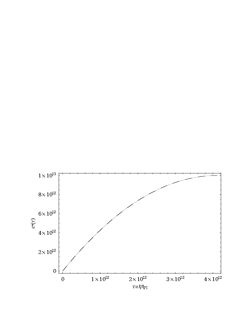
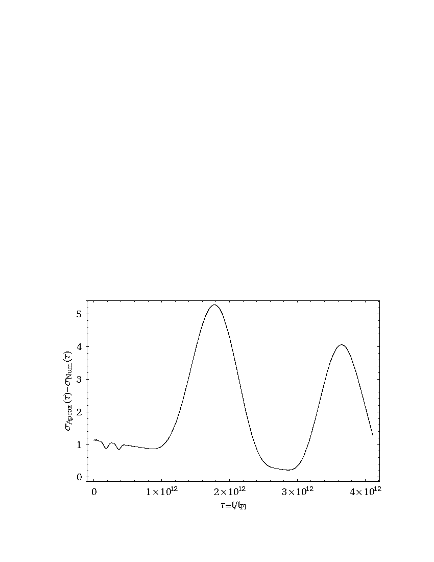
Figure 1: a) Top: The dashed line shows the numerical solution of $\sigma(\tau\equiv t/\sqrt{8\pi}\,t_{\rm Pl})$, using Eq.(15), for $\Lambda=0$, MSSM particle content and $\tilde{f}\simeq 10^{-13}$. The gray line shows the parabolic solution [Eq.(17)]. b) Bottom: The difference between the approximate $\sigma_{\rm Aprox}$ [Eq.(17)] and the numerical solution $\sigma_{\rm Num}$ [Eq.(15)]. The difference corresponds to approximately one part in $10^{13}$.

In a previous paper, a relatively large value for $\tilde{f}$($=10^{-6}$) was used as a strong test of the accuracy of the approximate solution Eq.(17). [6] The peak value of Eq.(17) with this value of $\tilde{f}$ was compared with the peak value of the numerical solution of Eq.(15) and found to differ by only one part in $10^{6}$. In Fig. 1 we plot $\sigma(\tau)$ vs $\tau(\equiv t/\sqrt{8\pi}\,t_{\rm Pl})$, where $t_{\rm Pl}=1/\sqrt{8\pi}M_{\rm Pl}\simeq 5.3\times 10^{-44}{\rm sec}$ is the Planck time, for $\tilde{f}\simeq 10^{-13}$ [Eq.(32)] for the numerical solution [Eq.(15)] and for the approximate parabolic solution [Eq.(17)]. The approximate parabolic and numerical solutions basically coincide. The two curves differ by one part in $10^{13}$, as seen in Fig. 1b. Thus, for any value of $\tilde{f}$ on the order of $10^{-6}$ or less, the approximate solution is extremely accurate. The numerical analysis confirms the parabolic dependence of Eq.(17) to a very high precision up to $H\sim M_{\ast}$, where $M_{\ast}$ is the scale when most of the sparticles decouple, the inequality in Eq.(13) changes sign, and inflation becomes unstable.

In $\S$ 3, we derive the reverse engineered inflaton potential that produces the approximate solution [Eq.(17)]. In the next section, we present the theory and method for constructing the potential. [10]

3 The effective potential of the modified Starobinsky model

Consider the dynamics of a Robertson Walker universe model with a classical scalar field $\phi(t)$, the inflaton and a non-interacting fluid. Following Ref. ellis1, we construct the potential $V(\phi)$ from the set of equations

$$V(\phi(t))=\frac{1}{(8\pi G)}\left(\dot{H}+3H^{2}\right)$$ (18)

and

$$\dot{\phi}^{2}=-\frac{1}{(4\pi G)}\dot{H}\,.$$ (19)

Using the above equations, we construct the potential of the MSM: From Eq.(17), the Hubble parameter is

$$H(t)=\frac{H_{a}}{\sqrt{8\pi G}}-\frac{1}{(8\pi G)}\frac{H_{a}^{2}\tilde{f}}{2}\,t\,.$$ (20)

Substituting Eq.(20) into Eq.(19), we obtain

$$t(\phi)=\pm\frac{(8\pi G)}{H_{a}\sqrt{\tilde{f}}}\left(\phi(t)-\phi_{0}\right),\,$$ (21)

where $\left|\phi_{0}\right|>\left|\phi\right|$. Choosing the positive sign in Eq.(21), we have $-\infty<\phi<0$. [10] Substituting Eq.(21) into Eq.(20),

$$H(\phi)=\frac{H_{a}}{\sqrt{8\pi G}}-\frac{H_{a}\sqrt{\tilde{f}}}{2}\left(\phi(t)-\phi_{0}\right)\,.$$ (22)

We can find $V(\phi)$ by substituting Eq.(22) into Eq.(18) or $V(t)$ substituting Eq.(20) into Eq.(18):

$$V(t)=\frac{1}{(8\pi G)}\left[-\frac{{H^{2}_{a}\tilde{f}}}{2(8\pi G)}+3\left(\frac{H_{a}}{\sqrt{8\pi G}}-\frac{{H^{2}_{a}\tilde{f}}}{2(8\pi G)}\,t\right)^{2}\right]\,.$$ (23)

In Fig. 2, we show the effective potential until the end of inflation as a function of $\tau\equiv t/\sqrt{8\pi}\,t_{\rm Pl}$, using $\tilde{f}\simeq 10^{-13}$ [Eq.(32)] and the MSSM particle content. The potential is negligible at the end of inflation ($V_{\rm end}/M^{4}_{\rm Pl}\simeq{H_{a}^{2}}\tilde{f}$).

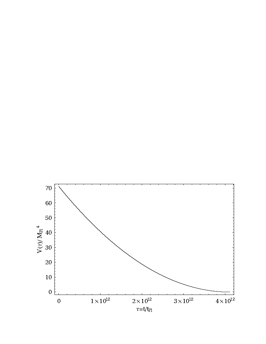
Figure 2: The potential [Eq.(23)] as a function of $\tau(\equiv t/\sqrt{8\pi}\,t_{\rm Pl})$ for $\tilde{f}\simeq 10^{-13}$ and the MSSM particle content.

The end of inflation occurs near the maximum of $\sigma(t)$, when $a(t)$ is no longer increasing exponentially with time at the mass (energy) scale $M_{\ast}$:

$$\dot{\sigma}(t){|}_{t=t_{\rm end}}=M_{\ast}\,.$$ (24)

We define the dimensionless parameter

$$\mu=M_{\ast}{\sqrt{8\pi G}}\,.$$ (25)

The time as a function of $\mu$ at the end of inflation is

$$t_{\rm end}=\frac{2\sqrt{8\pi G}}{H_{a}\tilde{f}}\left[1-\left(\frac{\mu}{H_{a}}\right)\right]\,.$$ (26)

Substituting $t_{\rm end}$ into Eq.(23), we have

$$V(t=t_{\rm end})/M^{4}_{\rm Pl}={H_{a}^{2}}\tilde{f}\,,$$

where $M_{\rm Pl}^{2}=1/(8\pi G)$. Since from Eq.(32) $\tilde{f}$ is small, $V(\phi)$ is small at the end of inflation, compared with its initial value.

The slow roll parameters in terms of the Hubble parameter are [22]

$$\epsilon\equiv 2\,M_{\rm Pl}\left[\frac{H^{\,\prime}\left(\phi\right)}{H\left(\phi\right)}\right]^{2}\,,$$

$$\eta\equiv 2\,M_{\rm Pl}\left[\frac{H^{\,\prime\prime}\left(\phi\right)}{H\left(\phi\right)}\right]\,.$$ (27)

The value for $\mu$, that characterizes the end of inflation is determined by the condition that the slow-roll parameter of inflation is $\epsilon=1$. Using this condition and Eqs.(22) and (27), we obtain

$$\mu\approx H_{a}\sqrt{\frac{\tilde{f}}{2}}\,.$$ (28)

The number of $e$-folds of inflation before $t=t_{\rm end}$ is

$$N=\int_{t_{60}}^{t_{\rm end}}H(t)dt=\sigma(t_{\rm end})-\sigma(t_{60})\,.$$ (29)

We are interested in $N\simeq 60$, the approximate time $t_{60}$ when the observed density (scalar) fluctuations and the primordial gravitational (tensor) fluctuations from inflation were created. Substituting $t_{\rm end}$ in Eq.(17), we find $\sigma_{\rm end}$. From (29), we get $\sigma_{60}$. Solving (17) for $t_{60}$, we obtain

$$t_{60}=\frac{2\sqrt{8\pi G}}{H_{a}\tilde{f}}\left[1-\sqrt{\left(\frac{\mu}{H_{a}}\right)^{2}+60\tilde{f}}\right]\,.$$ (30)

Substituting $t_{60}$ from Eq.(30) and $\mu$ from Eq.(28) into Eq.(23), we obtain the density fluctuations,

$$\frac{\delta\rho}{\rho}=2\,M_{\rm Pl}\,\frac{V^{{3}/{2}}(t)}{V^{\prime}(t){dt}/{d\phi}}|_{t=t_{60}}\approx 5.4H_{a}\sqrt{{\tilde{f}}/{2}}$$ (31)

that is observed to be $\approx 10^{-5}$. From the requirement that ${\delta\rho}/{\rho}\simeq 10^{-5}$, we find that

$$\tilde{f}\approx 2.05\times 10^{-13}\,.$$ (32)

Using this result in Eqs.(28) and (25), we obtain the scale

$$M_{\ast}\approx 4.5\times 10^{12}{\rm GeV}\,,$$ (33)

which is the value of the Hubble rate $H_{\ast}$ when the massive particles decouple. Particles decouple when their masses are of the order of the temperature or of order $H_{\ast}^{1/2}M_{\rm Pl}^{1/2}$, which gives

$$M_{\rm SUSY}\simeq\sqrt{M_{\ast}M_{\rm Pl}}\simeq 10^{15}{\rm GeV}\,.$$ (34)

This value is greater than the electroweak scale ($\sim 10^{3}{\rm GeV}$) and consistent with the predicted GUT scale ($\sim 10^{14}\,-\,10^{16}{\rm GeV}$).

4 Conclusions

A scalar potential was constructed using the approximate solution for the time dependence of the cosmological scale factor of the MSM during inflation. The potential was normalized at a time $\sim 60$ $e$-folds before the end of inflation in order to obtain the observed level of density fluctuations in the CMB, $\delta\rho/\rho\sim 10^{-5}$. The mass (energy) scale of the MSM at the end of the inflation, $M_{\ast}\simeq 10^{12}{\rm GeV}$, which we identify with the Hubble rate when the massive particles decouple, predicts a SUSY scale $M_{\rm SUSY}$, consistent with the GUT scale $M_{\rm SUSY}\simeq 10^{15}{\rm GeV}$.

References

- [1] M.V. Fischetti, J.B. Hartle, and B.L. Hu, Phys. Rev. D20, 1757 (1979).
- [2] A.A. Starobinsky, Phys. Lett. B91, 99 (1980); I.L. Buchbinder, S.D. Odintsov, and I.L. Shapiro, Phys. Lett B162, 92 (1985).
- [3] S.G. Mamaev and V.M. Mostepanenko, Sov. Phys. - JETP 51, 9 (1980).
- [4] J.C. Fabris, A.M. Pelinson, and I.L. Shapiro, Grav. Cosmol. 6, 59 (2000).
- [5] J.C. Fabris, A.M. Pelinson, and I.L. Shapiro, Nucl. Phys. B597, 539 (2001).
- [6] A.M. Pelinson, I.L. Shapiro, and F.I. Takakura, Nucl. Phys., B648, 417 (2003).
- [7] I.L. Shapiro, Int.J.Mod.Phys. D11, 1159 (2002).
- [8] I.L. Shapiro and J. Solà, Phys. Lett. B530, 10 (2002); E.V. Gorbar and I.L. Shapiro, JHEP 02, 021 (2003).
- [9] E.V. Gorbar, I.L. Shapiro, JHEP 02 (2003) 021.
- [10] G.F.R. Ellis, J. Murugan, and C.G. Tsagas, Class. Quant. Grav. 21, 233 (2004).
- [11] N.D. Birell and P.C.W. Davies, Quantum fields in curved space (Cambridge Univ. Press, Cambridge, 1982).
- [12] I.L. Buchbinder, S.D. Odintsov, and I.L. Shapiro, Effective Action in Quantum Gravity (IOP Publishing, Bristol, 1992).
- [13] R.J. Reigert, Phys. Lett. B134, 56 (1980).
- [14] E.S. Fradkin and A.A. Tseytlin, Phys. Lett. B134, 187 (1980).
- [15] R.D. Peccei, J. Solà, C. Wetterich, Phys. Lett. B195 183 (1987).
- [16] J.R. Ellis, N.C. Tsamis, M.B. Voloshin, Phys. Lett. B194 291 (1987).
- [17] C. Wetterich, Nucl. Phys. B302 668 (1988).
- [18] W. Buchmuller and N. Dragon, Nucl. Phys. B321 207 (1989).
- [19] J. Solà, Phys. Lett. B228 317 (1989); Int.J.Mod.Phys. A5 4225 (1990).
- [20] G.D. Coughlan, I. Kani, G.G. Ross, G. Segre, Nucl. Phys. B316 469 (1989).
- [21] E.T. Tomboulis, Nucl. Phys. B329 410 (1990).
- [22] A.R. Liddle and D.H. Lyth, Cosmological inflation and large-scale structure (Cambridge Univ. Press 2000).