CAIRNS: The Cluster And Infall Region Nearby Survey II. Environmental Dependence of Infrared Mass-to-Light Ratios

Abstract

CAIRNS (Cluster And Infall Region Nearby Survey) is a spectroscopic survey of the infall regions surrounding nine nearby rich clusters of galaxies. In Paper I, we used redshifts within $\sim 10h^{-1}{\rm Mpc}$ of the centers of the clusters to determine the mass profiles of the clusters based on the phase space distribution of the galaxies. Here, we use 2MASS photometry and an additional 515 redshifts to investigate the environmental dependence of near-infrared mass-to-light ratios. In the virial regions, the halo occupation function is non-linear; the number of bright galaxies per halo increases more slowly than the mass of the halo. On larger scales, the light contained in galaxies is less clustered than the mass in rich clusters. Specifically, the mass-to-light ratio inside the virial radius is a factor of $1.8\pm 0.3$ larger than that outside the virial radius. This difference could result from changing fractions of baryonic to total matter or from variations in the efficiency of galaxy formation or disruption with environment. The average mass-to-light ratio $M/L_{K}=53\pm 5h$ implies $\Omega_{m}=0.18\pm 0.03$ (statistical) using the luminosity density based on 2dFGRS data. These results are difficult to reconcile with independent methods which suggest higher $\Omega_{m}$. Reconciling these values by invoking bias requires that the typical value of $M/L_{K}$ changes significantly at densities of $\lesssim$3$\rho_{c}$.

1 Introduction

The relative distribution of matter and light in the universe is one of the outstanding problems in astrophysics. Clusters of galaxies, the largest gravitationally relaxed objects in the universe, are important probes of the distribution of mass and light. Zwicky (1933) first computed the mass-to-light ratio of the Coma cluster using the virial theorem and found that dark matter dominates the cluster mass. Recent determinations using the virial theorem yield mass-to-light ratios of $M/L_{B_{j}}\sim 250hM_{\odot}/L_{\odot}$ (Girardi et al., 2000, and references therein). Equating the mass-to-light ratio in clusters to the global value provides an estimate of the mass density of the universe (Oort, 1958); this estimate is subject to significant systematic error introduced by differences in galaxy populations between cluster cores and lower density regions (Carlberg et al., 1997; Girardi et al., 2000). Indeed, some numerical simulations suggest that cluster mass-to-light ratios exceed the universal value (Diaferio, 1999; Kravtsov & Klypin, 1999; Bahcall et al., 2000; Benson et al., 2000, but see also Ostriker et al. 2003).

Determining the global matter density from cluster mass-to-light ratios therefore requires knowledge of the dependence of mass-to-light ratios on environment. Bahcall et al. (1995) show that mass-to-light ratios increase with scale from galaxies to groups to clusters. Ellipticals have larger overall values of $M/L_{B}$ than spirals, presumably a result of younger, bluer stellar populations in spirals. At the scale of cluster virial radii, mass-to-light ratios appear to reach a maximum value. Some estimates of the mass-to-light ratio on very large scales ($>$10$h^{-1}{\rm Mpc}$) are available (see references in Bahcall et al., 1995), but the systematic uncertainties are large.

There are few estimates of mass-to-light ratios on scales between cluster virial radii and scales of 10$h^{-1}{\rm Mpc}$ (Eisenstein et al., 1997; Small et al., 1998; Kaiser et al., 2004; Rines et al., 2000, 2001a; Biviano & Girardi, 2003; Katgert et al., 2004; Kneib et al., 2003). On these scales, many galaxies near clusters are bound to the cluster but not yet in equilibrium (Gunn & Gott, 1972). These cluster infall regions have received relatively little scrutiny because they are mildly nonlinear, making their properties very difficult to predict analytically. However, these scales are exactly the ones in which galaxy properties change dramatically (Ellingson et al., 2001; Lewis et al., 2002; Gómez et al., 2003; Treu et al., 2003; Balogh et al., 2004, and references therein). Variations in the mass-to-light ratio with environment could have important physical implications; they could be produced either by a varying dark matter fraction or by variations in the efficiency of star formation with environment. In blue light, however, higher star formation rates in field galaxies compared to cluster galaxies could produce lower mass-to-light ratios outside cluster cores resulting only from the different contributions of young and old stars to the total luminosity (Bahcall et al., 2000).

Because clusters are not in equilibrium outside the virial radius, neither X-ray observations nor Jeans analysis provide secure mass determinations at these large radii. There are now two methods of approaching this problem: weak gravitational lensing (Kaiser et al., 2004) and kinematics of the infall region (Diaferio & Geller, 1997; Diaferio, 1999, hereafter DG97 and D99). Kaiser et al. (2004) analyzed the weak lensing signal from a supercluster at $z\approx 0.4$; the mass-to-light ratio ($M/L_{B}$=280 $\pm$40 $h$ for early-type galaxy light) is constant on scales up to $6~{}h^{-1}{\rm Mpc}$. Wilson et al. (2001) finds similar results for weak lensing in blank fields; Gray et al. (2002) obtain similar results for a different supercluster. Recently, Kneib et al. (2003) used weak lensing to estimate the mass profile of CL0024+1654 to a radius of 3.25$h^{-1}{\rm Mpc}$. Kneib et al. (2003) conclude that the mass-to-light ratio is roughly constant on these scales.

Galaxies in cluster infall regions produce sharp features in redshift surveys (Kent & Gunn, 1982; Shectman, 1982; de Lapparent et al., 1986; Kaiser, 1987; Ostriker et al., 1988; Regös & Geller, 1989). Early investigations of this infall pattern focused on its use as a direct indicator of the global matter density $\Omega_{m}$. Unfortunately, random motions caused by galaxy-galaxy interactions and substructure within the infall region smear out this cosmological signal (DG97, Vedel & Hartwick, 1998). Instead of sharp peaks in redshift space, infall regions around real clusters typically display a well-defined envelope in redshift space which is significantly denser than the surrounding environment (Rines et al., 2003, hereafter Paper I, and references therein).

DG97 analyzed the dynamics of infall regions with numerical simulations and found that in the outskirts of clusters, random motions due to substructure and non-radial motions make a substantial contribution to the amplitude of the caustics which delineate the infall regions (see also Vedel & Hartwick, 1998, and references therein). DG97 showed that the amplitude of the caustics is a measure of the escape velocity from the cluster; identification of the caustics therefore allows a determination of the mass profile of the cluster on scales $\lesssim 10h^{-1}{\rm Mpc}$.

DG97 and D99 show that nonparametric measurements of caustics yield cluster mass profiles accurate to $\sim$50% on scales of up to 10 $h^{-1}$ Mpc. This method assumes only that galaxies trace the velocity field. Indeed, simulations suggest that little or no velocity bias exists on linear and mildly non-linear scales (Kauffmann et al., 1999a, b). Geller et al. (1999, hereafter GDK), applied the kinematic method of D99 to the infall region of the Coma cluster. GDK reproduced the X-ray derived mass profile and extended direct determinations of the mass profile to a radius of $10~{}h^{-1}{\rm Mpc}$. The caustic method has also been applied to the Shapley Supercluster (Reisenegger et al., 2000), A576 (Rines et al., 2000, hereafter R00), AWM7 (Koranyi & Geller, 2000), the Fornax cluster (Drinkwater et al., 2001), A1644 (Tustin et al., 2001), A2199 (Rines et al., 2002), and six other nearby clusters (Paper I). Biviano & Girardi (2003) applied the caustic technique to an ensemble cluster created by stacking redshifts around 43 clusters from the 2dF Galaxy Redshift Survey. R00 found an enclosed mass-to-light ratio of $M/L_{R}\sim 300h$ within 4$~{}h^{-1}{\rm Mpc}$ of A576. Rines et al. (2001a) used 2MASS photometry and the mass profile from GDK to compute the mass-to-light profile of Coma in the K-band. They found a roughly flat profile with a possible decrease in $M/L_{K}$ with radius by no more than a factor of 3. Biviano & Girardi (2003) find a decreasing ratio of mass density to total galaxy number density. For early-type galaxies only, the number density profile is consistent with a constant mass-to-light (actually mass-to-number) ratio.

Here, we calculate the infrared mass-to-light profile within the turnaround radius for the CAIRNS clusters (Paper I), a sample of nine nearby rich, X-ray luminous clusters. We use photometry from the Two Micron All Sky Survey (2MASS, Skrutskie et al., 1997) and add several new redshifts to obtain complete or nearly complete surveys of galaxies up to 1-2 magnitudes fainter than $M^{*}_{K_{s}}$ (as determined by Kochanek et al., 2001; Cole et al., 2001, hereafter K01 and C01). Infrared light is a better tracer of stellar mass than optical light (Gavazzi et al., 1996; Zibetti et al., 2002); it is relatively insensitive to dust extinction and recent star formation. Despite these advantages, there are very few measurements of infrared mass-to-light ratios in clusters (Tustin et al., 2001; Rines et al., 2001a; Lin et al., 2003).

Mass-to-light ratios within virial regions (where the masses are more accurate than in the infall regions) provide interesting constraints on the distribution of dark matter and stellar mass (see also Lin et al., 2003, hereafter L03). The virial masses in our sample span an order of magnitude in mass. More massive clusters have larger mass-to-light ratios.

Cluster virial regions also provide potentially important constraints on the halo occupation distribution (e.g., Peacock & Smith, 2000; Berlind & Weinberg, 2002; Berlind et al., 2003, and references therein), the number of galaxies in a halo of a given mass (see Cooray & Sheth, 2002, for a recent review). The motions of galaxies and hot gas yield estimates of the dynamical mass independent of the number of galaxies (provided enough galaxies are present to yield a virial mass). Our mass profiles in Paper I are among the first to extend significantly beyond $r_{200}$. Thus, they should provide accurate estimates of $r_{200}$. Also, the recent release of 2MASS allows us to count galaxies based on their near-infrared light, which is close to selecting galaxies by stellar mass. Thus, both the masses and galaxy numbers are better defined than the few previous direct estimates of the halo occupation function (Peacock & Smith, 2000; Marinoni & Hudson, 2002; Lin et al., 2004).

We describe the cluster sample, the near-infrared photometry, and the spectroscopic observations in $\S$ 2. We discuss the galaxy properties (luminosity functions and broadband colors) within and outside the virial radius and compare both populations to field galaxies in $\S 4$. We calculate the number density and luminosity density profiles in $\S 5$ and compare them to simple theoretical models. We compute radial profiles of the mass-to-light ratio in $\S 5$. In $\S 6$ we constrain the halo occupation distribution for the CAIRNS clusters and explore the dependence of mass-to-light ratios on halo mass. We discuss possible systematic uncertainties and the implications of our results in $\S 7$ and conclude in $\S 8$. We assume a cosmology of $H_{0}=100~{}h~{}{\rm km~{}s}^{-1},\Omega_{m}=0.3,\Omega_{\Lambda}=0.7$ except as noted in $\S 7$.

2 Observations

2.1 The CAIRNS Cluster Sample

We selected the CAIRNS parent sample from all nearby ($cz<15,000~{}{\rm km~{}s}^{-1}$), Abell richness class $R\geq 1$ (Abell et al., 1989), X-ray luminous ($L_{X}>2.5\times 10^{43}h^{-2}$erg s^-1) galaxy clusters with declination $\delta>-15^{\circ}$. Using X-ray data from the X-ray Brightest Abell Clusters catalog (Ebeling et al., 1996), the parent cluster sample contains 14 systems. We selected a representative sample of 8 of these 14 clusters (Table 1). The cluster properties listed in Table 1 are from Paper I. The 6 clusters meeting the selection criteria but not targeted in CAIRNS are: A193, A426, A2063, A2107, A2147, and A2657. The 8 CAIRNS clusters span a variety of morphologies, from isolated clusters (A496, A2199) to major mergers (A168, A1367).

Table 1: CAIRNS Parent Population

Cluster	X-ray Coordinates		$cz_{\odot}$	$\sigma_{p}$	$L_{X}$	$T_{X}$	Richness
	RA (J2000)	DEC (J2000)	${\rm km~{}s}^{-1}$	${\rm km~{}s}^{-1}$	$10^{43}h^{-2}$ ergs s-1	keV
A119	00 56 12.9	-01 14 06	13268	698${}^{+36}_{-31}$	8.1	5.1	1
A168	01 15 08.8	+00 21 14	13395	579${}^{+36}_{-30}$	2.7	2.6	2
A496	04 33 35.2	-13 14 45	9900	721${}^{+35}_{-30}$	8.9	4.7	1
A539	05 16 32.1	+06 26 31	8717	734${}^{+53}_{-44}$	2.7	3.0	1
A576	07 21 31.6	+55 45 50	11510	1009${}^{+41}_{-36}$	3.5	3.7	1
A1367	11 44 36.2	+19 46 19	6495	782${}^{+56}_{-46}$	4.1	3.5	2
Coma	12 59 31.9	+27 54 10	6973	1042${}^{+33}_{-30}$	18.0	8.0	2
A2199	16 28 39.5	+39 33 00	9101	796${}^{+38}_{-33}$	9.1	4.7	2
A194	01 25 50.4	-01 21 54	5341	495${}^{+41}_{-33}$	0.4	2.6	0

Table 2: CAIRNS Hierarchical Centers

Cluster	Hierarchical Center		$cz_{cen}$	$cz_{CMB}$	$\Delta R$
	RA (J2000)	DEC (J2000)	${\rm km~{}s}^{-1}$	${\rm km~{}s}^{-1}$	$h^{-1}{\rm kpc}$
A119	00 56 10.1	-01 15 20	13278	12948	56
A168	01 15 00.7	+00 15 31	13493	13176	239
A496	04 33 38.6	-13 15 47	9831	9786	24
A539	05 16 37.0	+06 26 57	8648	8650	33
A576	07 21 32.0	+55 45 21	11487	11561	16
A1367	11 44 49.1	+19 46 03	6509	6837	61
Coma	13 00 00.7	+27 56 51	7096	7365	153
A2199	16 28 47.0	+39 30 22	9156	9181	86
A194	01 25 48.0	-01 21 34	5317	5011	11

The redshift limit is set by the small aperture of the 1.5-m Tillinghast telescope used for the vast majority of our spectroscopic observations. The richness minimum guarantees that the systems contain sufficiently large numbers of galaxies to sample the velocity distribution. The X-ray luminosity minimum guarantees that the systems are real clusters and not superpositions of galaxy groups (cf. the discussion of A2197 in Rines et al., 2001a, 2002). Three additional clusters with smaller X-ray luminosities (A147, A194 and A2197) serendipitously lie in the survey regions of A168 and A2199. A147 and A2197 lie at nearly identical redshifts to A168 and A2199; their dynamics are probably dominated by the more massive cluster (Rines et al., 2002). A194, however, is cleanly separated from A168 and we therefore analyze it as a ninth system. The inclusion of A194 extends the parameter space covered by the CAIRNS sample. The X-ray temperature of A194 listed in (Ebeling et al., 1996) is an extrapolation of the $L_{X}-T_{X}$ relation; in Table 1 we therefore list the direct temperature estimate of Fukazawa et al. (1998) from ASCA data. Fukazawa et al. (1998) lists X-ray temperatures for 6 of the 8 CAIRNS clusters which agree with those listed in Ebeling et al. (1996).

In Paper I, we applied a hierarchical clustering analysis (described in D99) to the redshift catalogs to determine the central coordinates and redshift of the largest system of galaxies in each cluster. Table 2 lists these hierarchical centers and their projected separations from the X-ray peaks. We adopt these hierarchical centers as the cluster centers.

2.2 2MASS Photometry

2MASS is an all-sky survey with uniform, complete photometry (Nikolaev et al., 2000) in three infrared bands (J, H, and K_s, a modified version of the K filter truncated at longer wavelengths). We use photometry from the final extended source catalog (XSC, Jarrett et al., 2000). The 2MASS XSC computes magnitudes in the $K_{s}$-band using several different methods, including aperture magnitudes (using a circular aperture with radius 7^′′), isophotal magnitudes which include light within the elliptical isophote corresponding to $\mu_{K_{s}}$=20 mag/arcsec², Kron magnitudes, and extrapolated “total” magnitudes (Jarrett et al., 2000). The sky coverage of the catalog is complete except for small regions around bright stars.

The 2MASS isophotal magnitudes omit $\sim$15% of the total flux of individual galaxies (K01). C01 compare 2MASS photometry from the Second Incremental Data Release (2IDR) with deeper infrared photometry from Loveday (2000). They find that Kron magnitudes are slightly fainter than the total magnitudes in deeper surveys (see also Andreon, 2002a) and that 2MASS extrapolated total magnitudes are slightly brighter than Kron (roughly total) magnitudes from the deeper survey. 2MASS is a relatively shallow survey and thus likely misses many low surface brightness galaxies Andreon (2002a); Bell et al. (2003). In this work we focus on bright galaxies (which typically have high surface brightness) so this bias is less important than, e.g., estimates of the luminosity density or stellar mass density.

Except where stated otherwise, we use the $K_{s}$-band survey extrapolated “total” magnitudes. Galactic extinction is usually negligible in the near-infrared. We correct for Galactic extinction by using the value in the center of the cluster. We make K corrections and evolutionary corrections of $<$0.15 magnitudes based on Poggianti (1997). Because these corrections are small and not strongly dependent on the galaxy model at the redshifts of the CAIRNS clusters, we apply a uniform correction for all galaxies in a given cluster interpolated from the model Elliptical SED with solar metallicity and a star-formation e-folding time of 1 Gyr.

We reprocess two galaxies in A576 and two galaxies near A2199 using the methodology of the 2MASS Large Galaxy Atlas (Jarrett et al., 2003). The galaxies in A576 (CGCG 261-056 NED01 and CGCG 261-056 NED 02) are bright ellipticals near the cluster center and also close to a bright star. One of the galaxies near A2199, UGC 10459, is an extremely flat edge-on disk galaxy. The other, NGC 6175, shows two nuclei aligned NW-SE. The SE component is brighter in $K_{s}$ band.

2.3 Spectroscopy

The 2MASS photometry allows selection of complete, near-infrared-selected samples extending $\sim$1-2 magnitudes fainter than the $M_{K_{s}}^{*}=-23.77+5\mbox{log}~{}h$ determined for the field galaxy luminosity function in 2MASS extrapolated magnitudes (C01). We define $K_{s}$-selected samples according to these magnitude limits within the smaller of the turnaround radius $r_{t}$ (the radius within which the average density is 3.5$\rho_{c}$) or the limiting radius $r_{max}$ of the caustic pattern (our membership criterion) in each cluster (see Paper I). Table 4 lists these radii and the apparent and absolute magnitude limits of these catalogs for the 9 clusters. Our redshift catalogs are 99.7% complete for cluster galaxy candidates brighter than $M_{K_{s}}=-23+5\mbox{log}h$ and 97.6% complete for candidates brighter than $M_{K_{s}}^{*}+1$.

Most of the galaxies in these samples have redshifts in the redshift catalogs from the CAIRNS project (Paper I). Between 2002 June and 2003 September, we collected new redshifts for 515 galaxies with the FAST spectrograph (Fabricant et al., 1998) on the 1.5-m Tillinghast telescope of the Fred Lawrence Whipple Observatory (FLWO). FAST is a high throughput, long slit spectrograph with a thinned, backside illuminated, antireflection coated CCD detector. The slit length is 180^′′; our observations used a slit width of 3^′′ and a 300 lines mm^-1 grating. This setup yields spectral resolution of 6-8 Å and covers the wavelength range 3600-7200 Å. We obtain redshifts by cross-correlation with spectral templates of emission-dominated and absorption-dominated galaxy spectra created from FAST observations (Kurtz & Mink, 1998). The typical uncertainty in the redshifts is 30$~{}{\rm km~{}s}^{-1}$. Table 3 lists the new redshifts. The additional redshifts make no significant difference to the locations of the caustics or to the resulting mass profiles. We thus use the caustics and mass profiles from Paper I.

Table 3: New Spectroscopic Data

RA	DEC	cz	$\sigma_{cz}$
(J2000)	(J2000)	(${\rm km~{}s}^{-1}$)	(${\rm km~{}s}^{-1}$)
00:46:06.30	-01:43:43.0	4074	16
00:46:34.60	-01:37:07.0	16888	40
00:47:12.60	-01:59:31.0	38906	40
00:50:46.10	-03:17:53.0	17204	23
00:53:05.60	-03:38:45.0	15993	41

Note. — The complete version of this table is in the electronic edition of the Journal. The printed edition contains only a sample.

An important difference between the FAST spectra collected for CAIRNS and those collected for other, larger redshift surveys (Colless et al., 2001; Stoughton et al., 2002) is that CAIRNS suffers no incompleteness due to fiber placement constraints.

We calculate the maximum fraction $f_{noz}$ of light missing from our catalogs if we assume that all galaxies without redshifts and brighter than the magnitude limit are cluster members (Table 4). In other words, we evaluate the potential observational bias which results if every galaxy without a redshift were a cluster member. For this extreme case, the total luminosity within $r_{max}$ is underestimated by the fraction $f_{noz}<0.10$ for all clusters. The new redshifts in Table 3 contribute significantly to the completeness of these catalogs. Because the galaxies without redshifts are almost entirely faint galaxies at large distances from the cluster center, $f_{noz}$ is a very conservative upper limit on the fraction of light missing within the completeness limits (the surface number density of member galaxies decreases with radius and the fraction of background galaxies increases with apparent magnitude).

Assuming that the luminosity function in clusters and infall regions is identical to that in the field (we test this assumption in $\S 3.1$), we calculate the fraction $f_{L}$ of total galaxy light contained in galaxies brighter than our completeness limits. This fraction is greater than 60% for all clusters. From repeated measurements, apparent magnitudes in the 2MASS XSC have an uncertainty of $\sim 0.14$ magnitude at $K_{s}=13.4-13.5$; the galaxy catalogs probably suffer incompleteness fainter than $K_{s}\approx 14$. Thus, the 2MASS XSC provides accurate magnitudes for galaxies within our completeness limits, but it is difficult to use 2MASS galaxy counts at much fainter magnitudes to estimate the contribution of fainter galaxies to the total cluster/infall region light. Note that the field luminosity function of C01 that we adopt here has a steeper faint-end slope than the luminosity function calculated from Kron magnitudes. If we adopt the Kron magnitude faint-end slope of C01, $f_{L}$ increases by 7-15% (the best sampled clusters have the smallest changes). We discuss this issue further in $\S 3.1$ and $\S 7.2$.

Figure 1 shows the redshift completeness as a function of apparent and absolute magnitude ($K_{s}$ extrapolated magnitude) along with the total number of galaxies, the number with redshifts, and the number of members versus magnitude. Note that, as in Paper I, we order the clusters by decreasing X-ray temperature from left to right and from top to bottom in this and all similar later figures. The catalogs are complete for cluster galaxy candidates brighter than $M_{K_{s}}=-23$ except for five candidates in the outskirts of A539 which lie at high Galactic extinction. It is not clear whether these objects are galaxies or extended Galactic infrared sources. The brightest of these sources, IRAS 05155+0707, is an embedded Class 1 protostar and likely the source of Herbig-Haro objects HH114 and HH115 (Reipurth et al., 1997). We exclude IRAS 05155+0707 from the photometric catalog and the calculation of $f_{noz}$ in Table 4.

Figure 1 also shows constraints on the luminosity functions in the clusters. The sets of dash-dotted lines show the limits from assuming that (1) all galaxies without redshifts are members or (2) none are. We discuss the luminosity functions in more detail in $\S 4$, but we note here that the faint-end slope of the luminosity function in infall regions is poorly constrained without deep, complete spectroscopy.

3 Properties of Galaxies Inside and Outside the Virial Region

Galaxy properties such as morphology and star formation rate are strongly correlated with their local and global environments (e.g., Ellingson et al., 2001; Lewis et al., 2002; Gómez et al., 2003; Treu et al., 2003; Balogh et al., 2004, and references therein). Differences in galaxy properties with environment may lead to apparent changes in the observed mass-to-light ratio even if the ratio of dark matter to stellar mass remains constant (e.g. Bahcall et al., 2000). The CAIRNS 2MASS selected galaxies provide a well-defined population with which to investigate these environmental effects. The environments considered range from cluster centers with densities $\sim$1000$\rho_{c}$ to the edges of infall regions with densities $\sim$3$\rho_{c}$ at the turnaround radius $r_{t}$. These environments are all denser than the universal average density $\Omega_{m}\rho_{c}$, but they cover the density range where galaxy morphologies, optical colors, and star formation rates change dramatically (Ellingson et al., 2001; Lewis et al., 2002; Gómez et al., 2003; Treu et al., 2003; Balogh et al., 2004). We investigate the near-infrared photometric properties of galaxies inside and outside the virial regions of the CAIRNS clusters and compare them to field galaxies.

3.1 Luminosity Functions

Many investigators have sought to determine the environmental dependence of the luminosity function (e.g., Balogh et al., 2001; Beijersbergen et al., 2002; De Propris et al., 2003, and references therein). Using the 2dF Galaxy Redshift Survey, De Propris et al. (2003) fit their cluster data to the Schechter (1976) luminosity function (LF),

$$N(M)\propto 10^{0.4(\alpha+1)(M^{*}-M)}e^{-10^{0.4(M^{*}-M)}}$$ (1)

and find that the cluster LF in the $b_{J}$ band has a brighter characteristic magnitude $M^{*}$ and steeper faint-end slope $\alpha$ than the field LF. Although differences between cluster and field luminosity functions exist at other wavelengths (e.g., Trentham, 1998a, b; Mobasher et al., 2003; Sabatini et al., 2003), the cluster LF in the $K_{s}$ band is quite similar to the field LF (e.g., Mobasher & Trentham, 1998; de Propris et al., 1998; Andreon & Pelló, 2000; Tustin et al., 2001; Balogh et al., 2001), perhaps indicating a universal stellar mass function (Andreon, 2004). Balogh et al. (2001) combine data from 2MASS and the Las Campanas Redshift Survey and find that the cluster LF in the $J$ band has a brighter characteristic magnitude and a steeper faint-end slope than the field LF; similar differences are seen at $K_{s}$ band but the parameters differ by $<$3-$\sigma$. Andreon (2004) finds that the cluster and field LFs are indistinguishable at red wavelengths in the optical (see also Christlein & Zabludoff, 2003), suggesting that much of the difference at bluer wavelengths is due to star formation.

Figure 2 shows the near-infrared luminosity functions of each of the CAIRNS clusters including all galaxies within the infall regions. We use the caustics from Paper I to define membership. In magnitude bins without complete redshifts, we compute a completeness correction by assuming that the membership fraction of galaxies without redshifts is the same as the membership fraction of galaxies with redshifts. Galaxies without redshifts tend to be at larger projected clustrocentric distances than those with redshifts. One might thus expect that these galaxies are more likely to be non-members because the ratio of cluster members to background galaxies decreases with radius. Counteracting this effect, galaxies without redshifts tend to have lower surface brightnesses than those with redshifts (because of observational bias towards higher surface brightness galaxies); because of the correlation between absolute magnitude and surface brightness, galaxies of a given apparent magnitude with lower surface brightnesses should be intrinsically fainter and are thus more likely to be cluster members (Conselice et al., 2002; Koranyi & Geller, 2000).

We count the number of bright galaxies (those with $M_{K_{s}}\leq M_{K_{s}}^{*}+1$) in each cluster and use this number to calculate relative normalizations for each cluster. Figure 2 shows the Schechter LF for field galaxies from C01 scaled by this number of bright galaxies with an arbitrary overall normalization.

We compute the luminosity functions separately for the virial regions and the infall regions taking $R_{200}$ ($r_{\delta}$ is the radius within which the enclosed mass density is $\delta$ times the critical density, $R_{\delta}=r_{\delta}$ is the projected radius) as the dividing radius. Some galaxies projected inside $R_{200}$ lie outside $r_{200}$, but no galaxies projected outside $R_{200}$ lie inside $r_{200}$; thus the luminosity functions inside $R_{200}$ will be contaminated by galaxies outside the virial region. Figure 3 shows the luminosity functions within $R_{200}$; Figure 4 shows the luminosity functions outside this radius. In each panel, we plot the best-fit Schechter (1976) luminosity function for field galaxies from C01 scaled by the number of bright galaxies with an arbitrary overall normalization. Figure 5 shows the combined CAIRNS LFs inside and outside $R_{200}$ as well as the total LF. The LFs in the virial regions and infall regions are very similar.

At the bright end, the LFs in both the virial regions and the infall regions are poorly fit by a Schechter function (Figure 5); the observed LFs contain more galaxies brighter than $M_{K_{s}}=-25$ and fewer galaxies at $-25<M_{K_{s}}\leq-24$ than a Schechter function which fits the faint-end slope. This difference may result from the existence and evolution of cD galaxies (e.g., Schombert, 1988; Tonry, 1987) present only in cluster environments. Figure 6 shows the ratio of the LF outside $R_{200}$ to that inside $R_{200}$. The infall region LF contains fewer extremely bright galaxies ($M_{K_{s}}\lesssim-25$) than the virial region LF, but there is very little difference within the Poissonian uncertainties. Also, it is worth noting that extremely bright galaxies are present in six of the nine infall regions (Coma, A119, A2199, A576, A168, and A194), demonstrating that these bright galaxies do not reside exclusively in cluster centers. Many of these galaxies likely occupy the centers of galaxy groups in the infall regions (Rines et al., 2001b). A $\chi^{2}$ test shows that the LF ratios for all bright galaxies ($M_{K_{s}}\leq-23.7$) are consistent with a constant value at the 95% confidence level.

At magnitudes fainter than the completeness limit, the LF in the infall region (excluding the virial region) consistently exceeds that inside the virial region, suggesting that the faint-end slope might be steeper in the infall region. The uncertainties in Figure 6 are Poissonian. Because the correction for galaxies without redshifts may be biased, these uncertainties may be significantly underestimated. A deeper complete spectroscopic survey of the infall regions is necessary to determine the reality of effects at these faint luminosities.

We calculate the best-fit luminosity function of the Schechter (1976) form for $M_{K_{s}}\leq-22.1+5\mbox{log}h$ for all the clusters combined. This limit corresponds to the 2MASS completeness limit of $K_{s}=13.5$ for the most distant CAIRNS clusters. We fit the LF for galaxies within $R_{200}$, outside $R_{200}$, and all galaxies combined. We do not account for measurement uncertainties in the fits. Table 5 lists the best-fit parameters (from minimizing $\chi^{2}$) as well as determinations of the field luminosity function (K01,C01). The uncertainties are 68% confidence limits for two interesting parameters. We list two different estimates from C01, one using extrapolated magnitudes (as used here) and one using 2IDR Kron magnitudes converted to ’total’ magnitudes by subtracting -0.20 mag (see C01). The LF parameters differ by 2-3$\sigma$ from the field values, and agree well with previous determinations (Balogh et al., 2001, L03). However, the fits to the CAIRNS LFs are not very good; the probability of obtaining a larger value of $\chi^{2}$ from a sample drawn from the Schechter LF is $<$0.7% for the total LF. The best-fit characteristic magnitude of the virial region LF is brighter than the field LF, similar both in sign and magnitude to the difference found by Balogh et al. (2001); the faint-end slope of the CAIRNS virial regions is slightly steeper than the field values. The LFs in the infall regions are intermediate between the field LFs and the virial region LFs.

We repeat the fits using the completeness limit of the redshift catalogs $M_{K_{s}}<-22.7$ and obtain consistent parameters with larger uncertainties due to the weaker constraints on the faint ends of the LFs. We experimented with different cuts in absolute magnitude both at the bright end (excluding cD-like galaxies that could skew the LF parameters) and the faint end. The best-fit LF parameters are fairly sensitive to the limiting magnitude adopted, perhaps because the cluster LF is not well described by a Schechter function. However, these parameters are generally within the 2-$\sigma$ range of the values listed in Table 5.

It is interesting that the characteristic magnitude of the CAIRNS virial region LF agrees well with that of the cluster LF constructed by L03 without spectroscopy. This agreement suggests that statistical background subtraction produces little bias in the resulting LF parameters. Both L03 and CAIRNS use 2MASS photometry which provides only a limited probe of the faint-end slope. It would be instructive to compare the LFs of individual clusters constructed with spectroscopic membership to those constructed with statistical background subtraction. A detailed comparison is outside the scope of the present work, but in $\S 5$ we will show that LFs constructed with statistical background subtraction (L03) yield mass-to-light ratios consistent with our results for clusters with complete spectroscopy.

The best-fit LF parameters significantly affect the estimates of the fraction of light $f_{L}$ contained in faint galaxies (see Table 4). However, for fixed LF parameters, the ratio of the maximum to the minimum values of $f_{L}$ for the clusters varies by less than 10%; thus, the relative values of $f_{L}$ are robust. Because the CAIRNS LF parameters are consistent with the field LF but have larger uncertainties, we continue to use the field LF to estimate the fraction of light contributed by faint galaxies. Note that the field LF we adopt (C01 extrapolated magnitudes) has both a brighter characteristic magnitude and a steeper faint-end slope than the LF of C01 from Kron magnitudes.

We repeat this analysis in the $J$ band, which extends deeper in 2MASS and thus has smaller statistical uncertainties. Figure 7 shows the J band LF for all galaxies within $r_{t}$, Figure 8 shows the luminosity functions within $R_{200}$, and Figure 9 shows the luminosity functions outside this radius. We combine the LFs to produce an average cluster LF in Figure 10. We scale the LF inside and outside $R_{200}$ to have the same normalization at $M_{J}^{*}$ for field galaxies. As in $K_{s}$ band, the cluster LF has a very similar shape to the field LF except for an excess of bright galaxies. We repeat the non-parametric test of computing the LF ratios (Figure 11). Table 5 lists the best-fit Schechter function parameters. These parameters differ by no more than 3-$\sigma$ from the field values determined by C01. The characteristic magnitude $M_{J}^{*}$ for cluster virial regions is brighter than the field value by about 0.5 magnitudes, consistent with the results of Balogh et al. (2001). There is remarkably little difference between the two LFs across the entire range of magnitudes, although at faint magnitudes there is room for significant differences which could be explored with deep, complete spectroscopy.

To summarize, we see marginal evidence for differences between the cluster LF and the field LF. The cluster LF is slightly brighter and has a steeper faint-end slope than the field LF. We obtain similar results in both $J$ and $K_{s}$ bands. Our data sample only giant galaxies, so significant differences may exist in the cluster and field LFs in the dwarf galaxy regime. For the purposes of computing mass-to-light ratios, the systematic uncertainty introduced by possible differences in the cluster and field LFs is $\lesssim 15\%$. Note that, as expected, the LF in the infall region is intermediate between the field LF and the cluster LF.

3.2 Luminosity Segregation

Dynamical friction could lead to luminosity segregation in galaxy clusters. Some investigators have claimed evidence for luminosity segregation in compilations of cluster data (e.g. Adami et al., 1998; Andreon, 2002b, and references therein). Figure 12 shows the distribution of absolute magnitude versus (projected) distance $R_{p}$ from the cluster center. If luminosity segregation were significant, we would see more bright galaxies near cluster centers. The brightest cluster galaxy is typically very close to the cluster center, consistent with a bright central cD galaxy increasing in mass through accretion of smaller galaxies. However, there are also many comparably bright galaxies in the outskirts of the clusters. In A2199, many of the extremely bright galaxies outside the virial region are at the centers of infalling groups (Rines et al., 2001b, 2002). There is little evidence for luminosity segregation in the CAIRNS clusters, consistent with earlier results for A576 (Rines et al., 2000). This result is not surprising given the similarity of the LFs inside and outside $R_{200}$ (Figure 5). Again, note that the CAIRNS samples do not extend into the dwarf galaxy regime, where luminosity segregation might be present (Andreon, 2002b).

3.3 Broadband Galaxy Colors

Star formation rates depend on environment (e.g., Ellingson et al., 2001; Lewis et al., 2002; Gómez et al., 2003; Treu et al., 2003; Balogh et al., 2004, and references therein). Because stellar populations in field galaxies are on average younger than those in cluster galaxies, more blue light is emitted per unit mass in field-like environments than in cluster environments. As a consequence, mass-to-blue-light profiles might decrease with radius (Bahcall et al., 2000) even if the ratio of gravitational mass to stellar mass were constant.

Because young stars are both hotter and bluer than older stars, the difference in stellar mass-to-light ratios decreases toward longer wavelengths (see the synthesized stellar population models of Bruzual & Charlot, 2003). For example, studies of near-infrared mass-to-light ratios in galaxies suggest that the mass-to-light ratio at these wavelengths is insensitive to the current star formation rate in either disk galaxies (Gavazzi et al., 1996) or early-type galaxies (Zibetti et al., 2002). Unfortunately, the color differences between J and K bands are not very large because these wavelengths primarily trace Population II stars (Jarrett et al., 2003), making this effect difficult to detect with 2MASS data alone.

For A576, our 9 square degrees of photometric CCD observations in R band (Rines et al., 2000) allow a measurement of $R-K_{s}$ colors. Optical-infrared colors enable us to investigate stellar population effects. Although both the 2MASS magnitudes used here and the R band magnitudes in Rines et al. (2000) are supposed to be close to total, a systematic difference in the magnitude definitions could introduce an artificial color gradient. We reprocess the R band images using SExtractor (Bertin & Arnouts, 1996) to obtain aperture magnitudes within a circular aperture of radius 14^′′  in R band and radius 15^′′ in 2MASS. This slight mismatch in apertures produces a small bias towards redder colors, but clustrocentric gradients, if any, should still be evident. We calculate $R-J$ and $R-{K_{s}}$ colors for all of the galaxies in both catalogs. Figure 13 displays the $R-{K_{s}}$ colors versus projected radius. There is no obvious radial gradient in either $R-J$ or $R-{K_{s}}$ colors for bright galaxies. There may be a radial gradient in $R-{K_{s}}$ colors for galaxies fainter than $M_{K_{s}}=-22.77$, but we lack complete spectroscopy at these magnitudes. In a photometric study of clusters using SDSS, Goto et al. (2004) find small but significant radial gradients in the fraction of blue galaxies with radius (the fraction increases with radius). The trends are weakest in the most nearby clusters which are the most similar to the CAIRNS clusters. Note that the CAIRNS catalogs are selected at $K_{s}$ rather than $r$, which may account for the lack of a gradient in A576. Also, the trends may be weaker in $R-{K_{s}}$ colors than in, e.g., $u-r$ colors, which are much more sensitive to the presence of young stars. A multiwavelength study of several clusters with spectroscopically determined membership would clarify the importance of color gradients in clusters.

We plot the $R-{K_{s}}$ color versus $K_{s}$ magnitude in Figure 14. There is little evidence for a color-magnitude relation. Galaxies inside and outside $R_{200}$ occupy the same parts of the diagram, indicating that there is no large difference in the two populations. The galaxies appear to have very similar stellar populations. Comparing the colors to the models of Bruzual & Charlot (2003) indicates metallicities greater than solar. The degeneracy between age and metallicity effects prevents further conclusions.

3.4 Near-Infrared Colors and the Color-Magnitude Relation

Significant variations in the stellar mass-to-light ratio might be indicated by radial gradients in $J-K_{s}$ colors. Unfortunately, identifying such gradients is difficult because variations in galaxy $J-K_{s}$ colors are relatively small and because unlike optical colors, galaxies with the reddest $J-K_{s}$ colors may contain younger stellar populations and are red as a result of emission from hot dust (Hunt et al., 2002; Barton Gillespie et al., 2003). We observe no radial color gradients in $J-K_{s}$ (see Figure 15, which highlights the lack of trends in the outlying points). Figure 16 shows that the distributions of $J-K_{s}$ colors of bright galaxies inside and outside $R_{200}$ are extremely similar. There is a possible excess of galaxies in the red tail of the distribution in the sample outside $R_{200}$ (Figure 15); some of these are edge-on disk galaxies while others are probably AGN (Jarrett, 2000; Jarrett et al., 2003). Because of the morphology-density relation, we expect more disk galaxies in cluster outskirts.

We plot $J-K_{s}$ color (computed within the elliptical isophote $K_{s}$=20 mag arcsec^-2) versus absolute magnitude $M_{K_{s}}$ (from the extrapolated $K_{s}$ magnitude) of CAIRNS members in Figure 17. The most striking result is that the outlying data points are galaxies both inside and outside $R_{200}$, which suggests that the stellar populations of galaxies in these regions are similar. There is tentative evidence for a color-magnitude relation (i.e., fainter galaxies are bluer, see, e.g., Terlevich et al., 2001, and references therein) in the near-infrared, but the slope ($\approx-0.01\mbox{mag}~{}\mbox{mag}^{-1}$) is much shallower than at optical wavelengths, e.g.,the slope is $-0.14\pm 0.01$ in $U-V$ versus $V$ in Coma (Terlevich et al., 2001). We obtain a similar color-magnitude relation when the colors and magnitudes are determined from aperture photometry, suggesting that the relation does not result from systematic effects in 2MASS. The variations in the colors can be explained by variations in the metallicities of the stellar populations. The most recent stellar population models of Bruzual & Charlot (2003) indicate that 10 Gyr old stellar populations (formed instantaneously according to a Chabrier (2003) initial mass function) with metallicities $[Fe/H]=-0.64\rightarrow+0.56$ have rest-frame $J-K_{s}=0.75\rightarrow 1.1$. As at optical wavelengths, there is degeneracy between age and metallicity effects; bluer colors result from either lower metallicities or younger ages (Worthey, 1994). Accurate spectral information is required to break this degeneracy (e.g., Concannon et al., 2000).

The scatter in the observed near-infrared color-magnitude relation is larger for fainter galaxies; the fainter galaxies have more varied stellar populations and/or larger uncertainties. Note that galaxies in clusters at low galactic latitude (A539 and A496) have larger scatter than those in clusters near the galactic poles (Coma and A1367). This observation suggests that a significant part of the scatter may result from uncertainties in Galactic extinction. A full accounting of the color-magnitude relation is beyond the scope of this paper. Instead, we note that the near-infrared properties of galaxies do not change dramatically with radius. This result implies that the stellar mass-to-light ratios do not change dramatically with radius; thus, measuring near-infrared mass-to-light ratios is a good approximation to a measurement of the ratio of total mass to stellar mass.

4 Near-Infrared Luminosity and Number Density Profiles

4.1 Number Density Profiles

Because our catalogs are essentially complete within their respective magnitude limits, we can count the number of bright galaxies to compare cluster richness. We adopt $M_{K_{s}}=-22.77+5\mbox{log}h$ as our limiting magnitude because all clusters are complete to this depth (Table 4). This limit is equivalent to $M_{K_{s}}^{*}+1$ for field galaxies. Table 6 lists the number of galaxies inside and outside $R_{200}$ (“outside $R_{200}$” means the projected radius $R_{p}$ satisfies $r_{200}<R_{p}\leq r_{max}$). In all clusters but A539, there are more cluster members outside $R_{200}$ than inside $R_{200}$. We suggested this result in Paper I but lacked the uniform photometry necessary to establish it.

Figure 18 shows the surface number density profiles of the CAIRNS clusters. We choose radial bins spaced logarithmically by 0.25; the outermost bin contains the maximum radius $r_{max}$ of the caustics. We fit the number density profiles of the CAIRNS clusters to three simple analytic models. The simplest model of a self-gravitating system is a singular isothermal sphere (SIS). The volume density of the SIS decreases with radius according to $\rho\propto r^{-2}$; the projected number density of objects $\Sigma$ decreases as $\Sigma(R_{p})\propto R_{p}^{-1}$. Navarro et al. (1997) and Hernquist (1990) propose two-parameter models based on CDM simulations of haloes. These density profiles are

$$\rho(r)\propto[\frac{r}{a}(1+\frac{r}{a})^{-\alpha}]$$ (2)

where $a$ is a scale radius and $\alpha$=2 for the NFW profile and $\alpha$=3 for the Hernquist profile. At large radii, the NFW density profile decreases as $r^{-3}$ and the density of the Hernquist model decreases as $r^{-4}$ (implying a finite total mass). The NFW surface number density profile is

$$\Sigma(<s)=\frac{N(a)}{\pi\mbox{ln}(4/e)a^{2}(s^{2}-1)}[1-X(s)]$$ (3)

where $s=R_{p}/a$ is the projected radius in units of the scale radius, $N(a)$ is the number of galaxies within the sphere of radius $a$, and

$$X(s)=\frac{\mbox{sec}^{-1}s}{\sqrt{s^{2}-1}}.$$ (4)

We fit the parameter $N(a)$ rather than the core density $n_{a}=3N(a)/(4\pi a^{3})$ because $N(a)$ and $a$ are much less correlated than $n_{a}$ and $a$ (Mahdavi et al., 1999). The Hernquist surface density profile is

$$\Sigma(<s)=\frac{2N(a)}{\pi a^{2}(s^{2}-1)^{2}}[(2+s^{2})X(s)-3]$$ (5)

where $a$ is the scale radius and $M$ is the total mass. Note that $M(a)=M/4$. We minimize $\chi^{2}$ and list the best-fit parameters $a_{N}$ for the NFW and Hernquist models in Table 7. We perform the fits on all data points within the maximum radii listed in Table 4. We plot the surface number density profiles and the best-fit NFW (solid lines) and Hernquist (dash-dotted lines) models in Figure 18. The SIS (dashed lines) is not normalized and is shown only for comparison.

The best-fit scale radii $a_{N}$ for both the NFW and Hernquist models are larger than the best-fit scale radii $a_{M}$ of the mass profiles in Paper I for all clusters except A539, where the NFW scale radius is the same. In individual clusters, $a_{N}$ and $a_{M}$ differ only at 1-3$\sigma$ significance. However, a K-S test indicates that the distributions of $a_{N}$ and $a_{M}$ are not drawn from the same population at the 99.6% confidence level for the NFW model and at 99.95% confidence for the Hernquist model. These differences suggest that mass is more concentrated than light.

Two clusters, A168 and A1367, are poorly fit by Hernquist and NFW profiles. They both could be fit by these profiles within $R_{200}$, but the surface number density outside $R_{200}$ exceeds the predicted profile. This result suggests that these clusters are not isolated from surrounding large-scale structure and that we may be observing them at an early stage of their evolution. In fact, both these clusters contain major mergers. Furthermore, they are the only CAIRNS clusters currently undergoing major mergers. Excluding these clusters from the comparison of scale radii only reduces the significance of the K-S test to 99.5% for both models. Thus, the difference in distribution of scale radii is not solely a result of these merging systems. Similarly, A2199 has a large core component. Excluding the innermost bin slightly increases the best-fit value of $a_{N}$ and slightly decreases the best-fit value of $N(a)$.

Biviano & Girardi (2003) find similar results from a Jeans analysis of an ensemble cluster constructed from the 2dFGRS: the ratio of mass density to galaxy (deprojected) number density decreases with radius. Similarly, Lin et al. (2004) find that the concentration of galaxies is smaller than the expected concentration of mass, i.e., the galaxies are more extended than expected. From our results and the independent analyses of these other authors, we thus conclude that the difference is a real physical effect.

4.2 Luminosity Profiles

Because the cluster LF is not significantly different from the field LF, the estimates of the fraction $f_{L}$ of the total cluster light contained in galaxies brighter than the magnitude limits in Table 4 (which assume the LF parameters of the field LF) are justified. We estimate the total light by adding the luminosity in galaxies brighter than the magnitude limits, then dividing by $f_{L}$. We make no corrections for the small incompleteness in our spectroscopic catalogs ($f_{noz}$ in Table 4). This omission could lead to slight underestimates of the luminosity in the outskirts of the clusters. The photometric uncertainties in the luminosity profiles are $\lesssim$10%. Because we compute the luminosity profiles only from relatively bright galaxies, the uncertainties are dominated by counting statistics (Kochanek et al., 2003).

We fit the luminosity density profiles of the CAIRNS clusters to the simple analytic models described in the previous section, replacing $N(a)$ with $L(a)$, the luminosity contained within the sphere of radius $a_{L}$. Figure 19 shows the surface luminosity density profiles and the best-fit NFW (solid lines) and Hernquist (dash-dotted lines) models. The scale radii $a_{L}$ of the light distributions are close to $a_{N}$ and larger than $a_{M}$, again implying that the light in galaxies is more extended than the mass. A K-S test indicates that the distributions of $a_{L}$ and $a_{M}$ are not drawn from the same population at the 98.1% confidence level for the NFW model and at 99.95% confidence for the Hernquist model. A K-S test detects no differences in the distributions of $a_{L}$ and $a_{N}$ for either model. Again we conclude that the mass is more concentrated than the light.

5 Near-Infrared Mass-to-Light Profiles

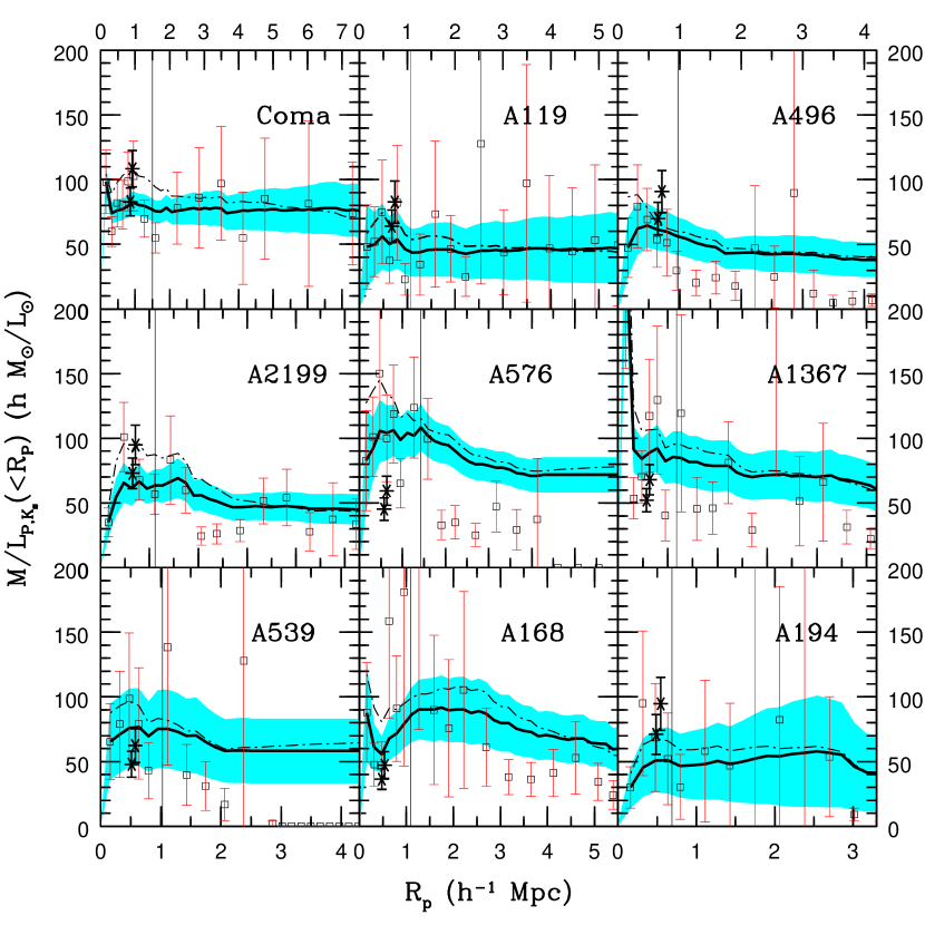
Figure 20: Mass-to-light ratio in $K_{s}$ band as a function of radius for the CAIRNS clusters. The solid lines show the caustic mass profile $M(<r)$ divided by the projected luminosity profile $L_{K_{s}}(<R_{p})$ and the shaded regions indicate the associated 1-$\sigma$ uncertainties. The open squares show the mass-to-light ratio $M(r,r+dr)/L_{K_{s}}(R_{p},R_{p}+dR_{p})$ in radial shells. The dash-dotted line shows the projected best-fit Hernquist mass profile $M_{H}(<R_{p})$ divided by $L_{K_{s}}(<R_{p})$. The stars show the mass-to-light ratio calculated using the X-ray temperature and the mass-temperature relation to estimate the mass. The lower point shows $M_{X}(<r_{500})/L_{K_{s}}(<R_{500})$ and the upper point shows $M_{X}(<R_{500})/L_{K_{s}}(<R_{500})$ assuming $M_{X}(<R_{500})=1.3M_{X}(<r_{500})$ as is true for an NFW mass profile with $c$=5.

We next compute $M(<r)/L_{K_{s}}(<R)$ as a function of radius (in units of $M_{\odot}/L_{\odot}$) using the caustic mass profiles and the luminosity profiles from the previous section (solid lines in Figure 20 with uncertainties shown in shading). The luminosity profiles $L_{K_{s}}(<R)$ are projected in two dimensions; the mass profiles $M(<r)$ are radial profiles. Thus, these mass-to-light profiles are the mass in spheres divided by the light in cylinders. Table 8 summarizes the mass-to-light ratios inside and outside $r_{200}$ calculated by dividing the caustic masses (in spheres) by the light profiles (in cylinders). Without correcting for this geometric effect, the mean mass-to-light ratio inside $r_{200}$ ($70\pm 7h$) is a factor of $1.8\pm 0.3$ larger than the mean mass-to-light ratio outside $r_{200}$ ($38\pm 6h$). The mean mass-to-light ratio inside the maximum radius probed, $r_{max}$, is $53\pm 5h$.

One notable feature of Figure 20 is the variety in the shapes of the mass-to-light profiles in individual clusters. Some clusters have flat profiles while others have strongly peaked profiles. There is no obvious cause of these differences (e.g., presence of a bright cD galaxy, presence of a major merger). Indeed, significant variation in the shapes of mass-to-light profiles obtained with the caustic technique is expected from projection effects along different lines of sight (D99).

Obviously, it is preferable to compute both the mass and the light in either spheres or cylinders but not one of each. Because mass and light are never negative, $L_{K_{s}}(<r)\leq L_{K_{s}}(<R_{p})$ and $M(<r)\leq M(<R_{p})$. Thus, this geometric effect should artificially decrease the “observed” mass-to-light ratios in the centers of the clusters. To correct for this geometric effect, one must make assumptions about the shapes of the profiles and their symmetries. We prefer to present the data with few manipulations. We thus project the mass profiles into cylinders rather than attempting to deproject the noisy luminosity profiles. In particular, we assume that the mass distribution is well-described by one of the simple mass models. Because the Hernquist profile has a finite total mass, the best-fit Hernquist profiles have smaller densities than the best-fit NFW profiles at large radii. Thus, the projected Hernquist profile is more centrally concentrated than the NFW profile. These projection effects will thus be larger if the true profile is a Hernquist profile. We show these projected $M_{H}(<R_{p})/L_{K_{s}}(<R)$ mass-to-light profiles as dash-dotted lines in Figure 20. As expected, these profiles have larger mass-to-light ratios at small radii than the spheres-by-cylinders profiles. If the decreasing shapes of these profiles are correct, the deprojected mass-to-light profiles $M(<r)/L(<r)$ should decrease slightly faster than in projection.

We quantify the size of this effect for NFW mass profiles. For NFW profiles with concentrations $c=5-20$ (in Paper I we measured $c=5-17$ for the CAIRNS clusters), the projected mass within a cylinder of radius $R_{200}$ is a factor of 1.15-1.25 larger than the mass in a sphere of radius $r_{200}$ (the factor increases with decreasing concentration). Projection effects are less dramatic for cylindrical shells compared to spherical shells at large radii because some light/mass outside the spherical shell is projected into the cylindrical shell; some light/mass within the spherical shell is projected into cylindrical shells at smaller radii. For NFW halos with concentrations $c=5-20$, the projected mass in the cylindrical shell bounded by $R_{200}$ and $R_{max}$ is 1–5% greater than the mass in the spherical shell bounded by $r_{200}$ and $r_{max}$. Thus, if the CAIRNS clusters are well-described by NFW profiles with $c\approx$5, the mass-to-light ratio inside the cylinder $R_{200}$ is larger by a factor of 1.15-1.25 than the measured quantity $M(<r_{200})/L(<R_{200})$. Similarly, the mass-to-light ratio in the cylindrical shell bounded by $R_{200}$ and $R_{max}$ is larger by a factor of 1.01-1.05 than the measured quantity $[M(<r_{max})-M(<r_{200})]/[L(<R_{max})-L(<R_{200})]$. The difference in mass-to-light ratios inside and outside $R_{200}$ is therefore larger than calculated above;

$$\frac{(M/L)(<R_{200})}{(M/L)(>R_{200})}\approx 1.2\frac{M(<r_{200})/L(<R_{200})}{M(>r_{200})/L(>R_{200})}\approx 2.2\pm 0.4.$$ (6)

The projection effects therefore aggravate the difference in mass-to-light ratios between cluster virial regions and their outskirts.

The preceding calculation used the nonparametric mass profiles from Paper I. We repeat the calculations of Table 8 using the best-fit (parametric) NFW mass profiles from Paper I projected into cylinders. The mean mass-to-light ratio inside $r_{200}$ is $M_{NFW}/L|_{r_{200}}=77\pm 7h$ and the mean mass-to-light ratio outside $r_{200}$ is $48\pm 5h$. The ratio of these is $1.6\pm 0.2$, very similar to the ratio $1.8\pm 0.3$ calculated above with no corrections for geometric projection effects. We note here that the best-fit NFW parameters do not vary significantly if the fits are restricted to $r<1.5~{}h^{-1}{\rm Mpc}$; at these radii, the mass profiles agree with X-ray and virial mass estimates (see Paper I).

We now calculate the mass-to-light profile in individual shells. The enclosed mass-to-light profiles calculated above decrease with radius. Because these profiles are dominated by the mass-to-light ratio in the core, the mass-to-light ratio in the outer shells must generally be smaller than the enclosed mass-to-light ratio at that radius. The uncertainties in individual shells are sufficiently large that we must bin several shells to obtain a significant signal. These mass-to-light ratios are the mass in spherical shells divided by the light in cylindrical shells. As noted above, for spherically symmetric NFW models, the projection effects decrease with radius and lead to underestimates of the mass-to-light ratio inside $r_{200}$. Open squares (Figure 20) show the mass-to-light ratios of these shells. Indeed, there is a general trend for lower mass-to-light ratios in shells at larger radii, but the uncertainties are quite large. Note that the enclosed mass-to-light profiles $M(<r)/L(<R_{p})$ are weighted by mass and light and therefore differ from the (unweighted) profiles of mass-to-light ratios in individual shells. For some clusters (e.g., Coma and A119), the mass-to-light ratios of shells at large radii agree well with the enclosed mass-to-light profile, while for others (e.g., A496 and A576) the mass-to-light ratios in shells at large radii are significantly lower than the enclosed mass-to-light profile. This variety is likely due to projection effects, namely the large variety in the appearance of the caustic pattern for an individual cluster viewed from different lines of sight (D99). This variety suggests that the shapes of individual mass-to-light profiles should not be taken too seriously; however, the average mass-to-light profile should be unbiased (D99).

X-ray mass estimates provide an independent check of our mass-to-light ratios within $r_{500}$. As shown in Paper I, the caustic mass profiles evaluated at $r_{500}$ agree quite well with X-ray mass estimates from the mass-temperature relation. Thus, it is no surprise that the mass-to-light ratios calculated from the X-ray mass $M_{500}$ and the luminosity evaluated at $L_{500}$ yield similar values. Note that, again, the luminosity estimates include all galaxies projected within $R_{500}$. An NFW profile with concentration $c$=5 appropriate for clusters (Navarro et al., 1997) would have a deprojected mass-to-light ratio $(M/L)(<r_{500})\approx 1.3M_{500}/L(<R_{500})$ (a higher concentration of $c$=20) reduces this factor from 1.3 to 1.2). We show both the projected and deprojected estimates as stars in Figure 20. Note that $(M/L)(<r_{500})\approx(M/L)(<R_{500})$; these points may be compared with the profiles of mass in cylinders divided by light in cylinders. The mean deprojected mass-to-light ratio is $(M/L)(<r_{500})=78\pm 7\mbox{(statistical)}hM_{\odot}/L_{\odot}$. This result agrees with the deprojected mass-to-light ratio $(M/L)(<r_{200})=88\pm 9h$ (statistical) at $r_{200}$ taken from the caustic mass profiles assuming a correction of 1.25 appropriate for a $c$=5 NFW halo. The agreement between the mass-to-light ratios within $r_{500}$ and within $r_{200}$ suggests that mass-to-light ratios are reasonably constant throughout the virial region of a cluster (see also $\S 6.2$). That is, the observed decrease in mass-to-light ratios with radius is not monotonic but may begin only at roughly $r_{200}$.

Our results are in excellent agreement with Lin et al. (2003, hereafter L03), who find a mass-to-light ratio $M/L_{K_{s}}=76\pm 4h$ (statistical) at $r_{500}$ for hot ($T_{X}\geq 3.7$keV) clusters using X-ray masses and 2MASS photometry from a larger cluster sample. We include only galaxies within the caustics in our luminosity estimates; L03 use statistical background subtraction to correct their luminosity estimates. The close agreement shows that the methods L03 use to subtract background galaxies do not introduce a bias in the luminosity estimates.

Previously, we have used the caustic technique to calculate mass-to-light profiles in R band for A576 (Rines et al., 2000) and in $K_{s}$ band for Coma (Rines et al., 2001a). In A576, we found a steeply decreasing mass-to-light profile in $R$ band. In Coma, we found a flat profile but noted that the systematic effects allowed for a decreasing profile. The results we derive here for these clusters are consistent with these earlier determinations.

Other investigators have applied Jeans analysis to ensemble clusters to test for variations in the mass-to-light ratio. This effort is complicated by the fact that one needs to assume an orbital distribution to measure variations in $M/L$. Carlberg et al. (1997) and van der Marel et al. (2000) find that light traces mass in the CNOC1 ensemble cluster (composed of massive clusters at $z=0.2-0.5$) to a radius of $2r_{200}$. Biviano & Girardi (2003) construct an ensemble cluster from poor clusters in the 2dFGRS. They find that the ratio of the mass density to the galaxy number density decreases with radius to $2r_{200}$, similar to our result for the CAIRNS clusters. When they exclude late-type galaxies from the galaxy number density, the ratio is roughly constant. Katgert et al. (2004) construct an ensemble cluster from the ESO (European Southern Observatory) Nearby Abell Cluster Survey and find that the mass-to-light ratio decreases with radius in the range $0.2-1.5r_{200}$, although the mass-to-light ratio is roughly constant when late-type galaxies are excluded.

Weak lensing provides an independent estimate of mass-to-light ratios on large scales that does not depend on the dynamical state of the system. Kaiser et al. (2004) and Gray et al. (2002) estimate the mass-to-light ratios of superclusters with weak lensing. Kaiser et al. (2004) find $M/L_{B}=280\pm 40h$ for light in early-type galaxies. Assuming a typical early-type color of $B-K_{s}=3.7$ (Jarrett, 2000), this value corresponds to $M/L_{K_{s}}\approx 64\pm 9h$. Including late-type galaxies would decrease this ratio. Wilson et al. (2001) find similar results from weak lensing in blank fields. Gray et al. (2002) find $M/L_{B}\sim 200h$ (early-type light only) for individual clusters; when they cross-correlate mass and light they find $M/L_{B}=130h$ (early-type light only), but they caution that there are many systematic uncertainties in this estimate. Recently, Kneib et al. (2003) used weak lensing to estimate the mass profile of CL0024+1654 to a radius of 3.25$h^{-1}{\rm Mpc}$. Kneib et al. (2003) conclude that the $K$ band mass-to-light ratio is roughly constant on these scales. Assuming passive evolution, their mass-to-light ratio corresponds to $65\pm 9h$ ($74\pm 10h$ for red sequence galaxies only) at $z=0$, intermediate between our estimates of the mass-to-light ratio inside and outside $r_{200}$.

Bahcall et al. (2000) use simulations to show that cluster mass-to-light ratios in B band exceed the global value due to the older, less luminous stellar populations found in clusters. Cluster mass-to-light ratios measured in $K_{s}$ band should then be much closer to the global value because $K_{s}$ band light has a much weaker dependence on stellar population ages (e.g., Bell & de Jong, 2001). If stellar populations are the primary cause of the decreasing mass-to-light profiles in the simulations of Bahcall et al. (2000), the CAIRNS clusters should have roughly flat $K_{s}$ band mass-to-light profiles. Thus, the similarity of the decreasing $K_{s}$ band mass-to-light profiles of the CAIRNS clusters to the simulations of Bahcall et al. (2000) shows that the decreasing profiles in their simulations may not result primarily from differences in the stellar populations but from differences in the relative distribution of dark matter and galaxies.

The CAIRNS sample is unique in both the completeness of the individual cluster catalogs and in the near-infrared digital photometry used to avoid stellar population effects. The mass-to-light ratios of the CAIRNS clusters decrease with radius and the mass-to-light ratios inside the virial regions agree with other estimates at optical and near-infrared wavelengths (see also Rines et al., 2000, 2001a). The decreasing mass-to-light profiles are consistent with results from other cluster studies. We discuss these results in more detail in $\S 7$.

6 Properties of the Virial Regions

6.1 The Halo Occupation Distribution

The halo occupation distribution (see the review by Cooray & Sheth, 2002) is an important input for converting the results of numerical simulations into observables (e.g., Peacock & Smith, 2000; Berlind & Weinberg, 2002; Berlind et al., 2003, and references therein). The simplest prediction is that the number of galaxies formed is directly proportional to the available baryonic mass. Thus, the number of galaxies $N$ (brighter than some minimum mass or luminosity) contained in a halo of mass $M$ is given by $N\propto M$ (i.e., the efficiency of galaxy formation is a universal constant for sufficiently massive haloes). If galaxy formation is more efficient in the most massive haloes, then the relation might be $N\propto M^{\mu}$ with $\mu>1$. Conversely, if galaxy formation is less efficient in massive haloes (e.g., if the gas is heated by the halo potential and is unable to collapse into galaxies) or galaxy disruption is more efficient (e.g., dynamical friction and tidal stripping), then the relation might be $N\propto M^{\mu}$ with $\mu<1$. Models of the halo occupation distribution suggest that, for cluster mass halos, the relation is close to a power law with slope $\mu<1$. Semi-analytic models predict $\mu\sim 0.8-0.9$ (Sheth & Diaferio, 2001; Berlind et al., 2003). A smoothed particle hydrodynamics simulation of a $\Lambda$CDM cosmological model predicts halo occupation distributions with $\mu\sim 0.56-0.74$ for cluster mass halos, similar to the values for a different set of semi-analytic models (Berlind et al., 2003). Springel & Hernquist (2003) show that numerical simulations predict suppression of galaxy formation in the most massive halos because gas cannot cool and collapse into galaxies.

One of the few previous determinations of the relation between virial masses and galaxy numbers is that of Marinoni & Hudson (2002), who compute masses and (blue) luminosities of virialized objects in the Nearby Optical Catalog. Marinoni & Hudson (2002) find $N\propto M^{0.55\pm 0.03}$, similar to the semi-analytic models. Kochanek et al. (2003) use a constrained numerical simulation of 2MASS to develop a matched filter algorithm to study cluster properties in the 2MASS catalog and heterogeneous auxiliary observations from the literature (e.g., redshifts and X-ray properties). Their best-fit relation between cluster mass and number of members is $N\propto M^{1.10\pm 0.09}$. Pisani et al. (2003) find $N\propto M^{0.70\pm 0.04}$ in a sample of groups, although mass estimates of groups are very uncertain. Recently, Lin et al. (2004) analyzed the halo occupation distribution for clusters with 2MASS photometry and X-ray mass estimates. They find $N\propto M^{0.84\pm 0.04}$, steeper than Marinoni & Hudson (2002) but still in reasonable agreement with models.

We can constrain the halo occupation distribution with the CAIRNS clusters, which cover roughly an order of magnitude in mass and have both accurate photometry and complete spectroscopy. Our results have the advantages of uniform sky coverage, greater redshift completeness, and galaxy selection at near-infrared wavelengths, which is a better tracer of stellar mass and suffers less dust extinction than blue light. Conveniently, the magnitude limit we adopt ($M_{K_{s}}\leq M_{K_{s}}^{*}+1$) is very similar to the luminosity threshold used in Berlind & Weinberg (2002) and one of the thresholds used in Berlind et al. (2003), $L\gtrsim 0.5L_{*}$. Figure 21 shows the number of galaxies $N_{200}$ projected within $R_{200}$ versus $M_{200}$, the mass of the halo. We do not attempt to deproject the number density profiles to obtain a deprojected estimate of $N_{200}$ because the number density profiles are too noisy. If all haloes have similar concentrations, then the fraction of interlopers should be constant with mass. If the halo concentration decreases with mass (as expected for NFW models), then the fraction of interlopers should increase with mass. In this case, the fit to $\mu$ would be an overestimate. The bisector of the two ordinary least-squares fits (Feigelson & Babu, 1992) yields $N_{200}\propto M_{200}^{0.70\pm 0.09}$, 3.3$\sigma$ shallower than a linear relation (shown by a dashed line in Figure 21). This result is not driven by A194, the least massive cluster; excluding this cluster yields a least squares fit $N_{200}\propto M_{200}^{0.74\pm 0.15}$. This result agrees well with previous determinations as well as with expectations from semi-analytic models for galaxy formation (e.g., Kauffmann et al., 1999a; Sheth & Diaferio, 2001; Marinoni & Hudson, 2002; Berlind et al., 2003; Pisani et al., 2003; Lin et al., 2004). We speculate that the significant difference from Kochanek et al. (2003) is due to the systematic uncertainties from the process of matching their simulation to the observations. Kochanek et al. (2003) use a matched filter algorithm which is finely tuned to reproduce the expected properties of clusters based on simulations (where galaxies trace the dark matter distribution). Systematic effects can arise both from mismatches in the assumed and true cosmology and recipes for galaxy formation as well as unknown systematics in the heterogeneous auxiliary observations.

The comparison with Lin et al. (2004) is especially interesting because both datasets use 2MASS photometry. Lin et al. (2004) use a much larger sample of clusters but they use only statistical background subtraction whereas we study fewer clusters but use complete spectroscopic information to assign cluster membership. A detailed comparison of these two methods would be instructive but it lies beyond the scope of this paper. In particular, there are few clusters in both samples, so cluster-to-cluster variations could significantly affect the comparisons. We refer the reader to Lin et al. (2004) for an excellent discussion of the physical significance of a non-linear HOF as well as the observational implications for clusters.

6.2 Mass Dependence of Mass-to-Light Ratios

Figure 22 shows the mass-to-light ratio within $r_{200}$ versus $M_{200}$ for the CAIRNS clusters. The scatter is large, but the CAIRNS clusters show an increase in M/L (evaluated at $r_{200}$) with increasing mass. Lin et al. (2003, hereafter L03) found a similar correlation between X-ray mass and near-infrared mass-to-light ratios; more massive clusters have larger mass-to-light ratios with a best-fit relation

$$(M/L_{K_{s}})(<r_{500})=(67\pm 4)h(\frac{M_{500}}{2.1\times 10^{14}h^{-1}M_{\odot}})^{0.31\pm 0.09}.$$ (7)

Figure 22 shows this relation assuming that the mass-to-light ratios within $r_{500}$ and $r_{200}$ are identical, $M_{200}\approx 3M_{500}$, and multiplying by 0.8 to convert to the spheres-by-cylinders measured here. The CAIRNS clusters follow this relation quite closely, showing that the mass estimator used (X-ray versus virial/caustic mass) does not affect the correlation of mass-to-light ratio with cluster mass. The close agreement also demonstrates that cluster mass-to-light ratios do not change dramatically between $r_{500}$ and $r_{200}$ (see also $\S$ 5).

A compilation of virial masses and luminosities by Girardi et al. (2000) yields $(M/L_{B_{j}})\propto M^{0.17-0.23}$ Similarly, Bahcall & Comerford (2002) use a heterogeneous catalog to derive a dependence of (optical) M/L on X-ray temperature which they attribute to differences in the ages of stellar populations. One can convert their relation into a $M/L-M$ relation with the X-ray mass-temperature relation (Finoguenov et al., 2001). Specifically, $(M/L)\propto T_{X}^{0.30\pm 0.08}$ and $M\propto T_{X}^{1.64\pm 0.04}$ yield $(M/L)|r_{200}\propto M_{200}^{0.18\pm 0.05}$, slightly shallower than but in agreement with the L03 relation and the CAIRNS clusters (Figure 22). Note, however, that the CAIRNS relation has little dependence on the ages of the stellar populations, counter to the conclusion of Bahcall & Comerford (2002). If differences in stellar populations produce the $M/L-M$ relation, the slope of the relation should be steeper for $M/L_{B}$ than for $M/L_{K_{s}}$.

In contrast, Kochanek et al. (2003) find that mass-to-light ratios are smaller in more massive clusters; they find a best-fit relation of $(M/L_{K_{s}})(<r_{200})=116\pm 46(M_{200}/10^{15}h^{-1}M_{\odot})^{-0.10\pm 0.09}$. We multiply this relation by 0.8 to convert to the spheres-by-cylinders measured here (Figure 22). The CAIRNS clusters follow the relation found by L03, Girardi et al. (2000), and Bahcall et al. (2000), and exclude the relation of Kochanek et al. (2003). The disagreement with Kochanek et al. (2003) is perhaps not surprising given the disagreement between their halo occupation function and that of the CAIRNS clusters found in the previous section.

Figure 23 shows the relation between $L_{200}$, and $N_{200}$, the number of bright galaxies ($M_{K_{s}}<-22.77+5\mbox{log}h$) projected within $R_{200}$. The bisector of the ordinary least-squares fits is $N_{200}\propto L_{200}^{0.93\pm 0.07}$, consistent with a slope of unity. This result underscores the result of $\S 3.1$; the cluster-to-cluster variations in the LF are small. Galaxy formation is suppressed (and/or that the efficiency of galaxy disruption is enhanced) in massive clusters, with greater suppression for more massive clusters. The correlation of mass-to-light ratio with mass is then a natural byproduct of the correlation of $M_{200}/N_{200}$ with mass and a universal LF.

These results are consistent with the decreasing mass-to-light profiles found in $\S 5$. These decreasing profiles imply that cluster infall regions, which contain galaxies formed in environments with smaller virial temperatures than galaxies in the virial regions, have smaller mass-to-light ratios. The presence of X-ray groups in cluster infall regions (Rines et al., 2001b, 2002) demonstrates the overlap between cluster infall regions and low-mass clusters. In $\S 6.1$, we show that the number of galaxies within $R_{200}$ increases more slowly than the cluster mass. These results all suggest that the efficiency of galaxy formation is suppressed (see the numerical simulations by Springel & Hernquist, 2003) and/or that the efficiency of galaxy disruption is enhanced (see the numerical simulations by Kravtsov & Klypin, 1999; Colín et al., 1999) in environments with larger virial temperatures. In the latter case, the contribution of intracluster stars to the cluster light budget can be substantial (5-50%, see $\S 7.4$). Neglecting this contribution (the normal procedure and the one adopted here) may result in a severe underestimate of the total light in the cluster.

7 Discussion

7.1 Predicting Mass Profiles From the Galaxy Distributions

Because the caustic technique is relatively new, we test the consistency of our results with velocity dispersion profiles (VDPs), a more traditional tool of galactic dynamics. Here we predict the mass profiles based on the observed distribution of galaxies assuming that they trace the mass. If the radial variations in the mass-to-light ratio ($\S 5$) are real, then the mass profiles calculated from the galaxy distributions (either number density or luminosity density) assuming a constant mass-to-light ratio should differ demonstrably from those in Paper I. We reproduce the VDPs from Paper I in Figure 24 (dash-dotted lines).

In $\S 4.1$ above, we fit the surface number density profiles of the bright galaxy distribution. The scale and normalization of the profiles predict the shape of the velocity dispersion profiles (VDPs) of the clusters under the assumption of isotropic orbits and a (globally) constant ratio $M/N$ of mass to number of bright galaxies ($M_{K_{s}}<-22.77+5\mbox{log}h$). We calculate the value of this ratio within $r_{200}$ and find $(M/N)|_{r200}=(7.8\pm 0.8)\times 10^{12}h^{-1}M_{\odot}\mbox{galaxy}^{-1}$. Figure 24 displays these predicted VDPs (solid lines) along with the observed VDPs and the VDPs of the best-fit Hernquist mass profiles from Paper I (dash-dotted lines). As noted in Paper I, the VDPs predicted by the caustic mass profiles agree well with the observed VDPs. The VDPs predicted from the surface density profiles, however, do not agree with the observed VDPs, especially in Coma and A576, where the predicted VDPs lie substantially below the observations.

This disagreement may result from anisotropic orbits or from cluster-to-cluster variations in $M/N$ (we find such variations in $\S 6.1$). Anisotropic orbits would affect both the shapes and normalizations of the predicted VDPs, but variations in $M/N$ only affect the normalizations (assuming that $M/N$ is constant with radius in each cluster). Figure 23 shows that $(M/N)|_{r200}$ increases with $M_{200}$. Correcting for this trend reconciles some of the differences in Figure 24, i.e., the most discrepant clusters are those with the highest masses. Substituting a higher $(M/N)|_{r200}$ increases the amplitude of the predicted VDPs and brings the predicted and observed VDPs into better agreement. Outside $r_{200}$, galaxies are not relaxed. At these radii, VDPs do not necessarily contain information about the orbital distribution. Thus, the VDPs outside $r_{200}$ should not be considered strong constraints on the mass and orbital distributions.

The most straightforward predictions of VDPs based on the assumption that light traces mass disagree with the observed VDPs. In contrast, the VDPs predicted by the caustic mass profiles agree well with the observed VDPs. Thus, the decrease in the efficiency of galaxy formation (and/or the increase in the efficiency of galaxy disruption) for haloes with larger virial temperatures is not an artifact of the caustic technique. Velocity dispersion profiles, a more traditional tool of galactic dynamics, also indicate a discrepancy between the distribution of galaxies and mass (although subject to possible biases from the orbital distribution and/or the dynamical state of galaxies outside $r_{200}$). It is interesting that Katgert et al. (2004) also find a decreasing mass-to-light profile for an ensemble cluster using Jeans analysis to compute the mass profile. Their results strengthen our conclusion that the decreasing mass-to-light profiles are physical effects.

7.2 Morphological Gradients

Because of the well-known correlation between morphology and density, we expect larger fractions of late-type galaxies with increasing clustrocentric radius (decreasing density). If the LFs of early-type and late-type galaxies differ significantly, the total LF should vary with clustrocentric radius. That is, the LF in cluster centers should closely resemble the early-type LF, whereas at larger radii it should resemble the late-type LF. K01 separate the LF into early-type and late-type LFs and find that fits to Schechter functions yield a brighter $M_{K_{s}}^{*}$ for the early-type LF; the faint-end slope is slightly shallower for the late-type LF (but see Bell et al., 2003, who find that 2MASS misses many blue low surface brightness galaxies present in SDSS).

Because our spectroscopic surveys extend to fixed absolute magnitudes, the correction for light in galaxies fainter than our limiting magnitudes changes with radius. Adopting the type-dependent LFs of K01, the correction becomes larger with radius provided the limiting magnitude is $M_{K_{s}}\lesssim-10$ (note that the type-dependent LFs are only constrained for $M_{K_{s},iso}\leq-20.5$). That is, a magnitude-limited survey misses more light at large clustrocentric radii. If the fraction of early-type galaxies changes from 1 to 0 (a huge overestimate), the correction changes by $\sim$20% ($\sim$10%) for a magnitude limit of $M_{K_{s},iso}$=-22.5 (-21.5), approximately the magnitude limits for the CAIRNS clusters. Correcting for this effect in $\S 5$ would add even more light to the cluster outskirts and lead to more steeply decreasing profiles. Thus, the decreasing mass-to-light profiles in $\S 5$ cannot be explained by the morphology-density relation.

7.3 Stellar Populations and Correcting for Faint Galaxies

Profiles of the ratio of dark matter to stellar mass can be used both to estimate $\Omega_{m}$ and to constrain prescriptions for galaxy formation. If $K_{s}$-band light traces stellar mass exactly, the results of $\S 5$ indicate that the efficiency of star formation is reduced in dense cluster environments. However, the properties of galaxies change rapidly with increasing distance from cluster centers (Balogh et al., 2004, and references therein). In particular, the stellar mass-to-light ratio is smaller in late-type galaxies than in early-type galaxies by up to a factor of two. Late-type galaxies are much more common in the field than in clusters. Thus, the mean stellar mass-to-light ratio should decrease with radius.

Because stellar populations are younger at larger clustrocentric radii, mass-to-optical-light profiles might decrease with radius (Bahcall et al., 2000) even if the ratio of gravitational mass to stellar mass is constant. Thus, the total-to-stellar mass profiles of the CAIRNS clusters may decrease less steeply than the mass-to-light profiles. Here, we test for radial gradients in the stellar mass-to-light ratio in A576 and estimate the magnitude of this effect in $K_{s}$ band.

7.3.1 A Test in A576 and the Importance of Faint Galaxies

We showed above ($\S 3.3$) that there are no obvious gradients in the $R-K_{s}$ colors of galaxies in A576. We test for gradients in the stellar mass-to-light ratio directly by comparing the mass-to-light profiles in an optical band (R) and near-infrared bands. If there were a significant gradient in stellar mass-to-light ratios, the near-infrared profile would be flatter than at optical wavelengths.

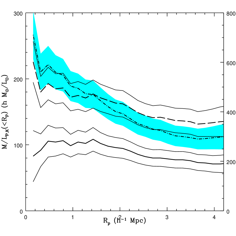
Figure 25: Comparison of $K_{s}$ band and $R$ band mass-to-light profiles for A576. The vertical scale on the right is for $R$ band. The $K_{s}$ band mass-to-light profile is the lower set of solid lines with 1-$\sigma$ uncertainties. The dash-dotted line and shaded region show the $R$ band mass-to-light profile and 1-$\sigma$ uncertainties from Rines et al. (2000). The dashed line shows the $R$ band mass-to-light profile and surrounding solid lines show the 1-$\sigma$ uncertainties calculated from bright galaxies assuming a constant fraction of light in fainter galaxies.

Indeed, the ${K_{s}}$ band mass-to-light profile (thick solid line in Figure 25) decreases more slowly than the R band profile (dash-dotted line). The cumulative mass-to-light ratio decreases by a factor of $\sim$2 in R band and by a factor of $\sim$1.4 in $K_{s}$ band. This result suggests that the effect of star formation gradients on mass-to-light profiles is significant in the R band as well as in the B band (e.g., Bahcall et al., 2000). However, there is no obvious change in the average $R-{K_{s}}$ color with radius in A576 ($\S 3.3$). Thus, the steeper decrease in the cumulative mass-to-light profile in the $R$ band is not readily explained by a simple color gradient.

Another explanation for the difference in $R$ and $K_{s}$ band $M/L$ profiles is the corrections for faint galaxies without redshifts. The R band catalog has complete spectroscopy to R=16.5 and complete photometry to R=18.0. Rines et al. (2000) used several techniques to estimate the (assumed constant) flux surface density contributed by background galaxies. Here, by contrast, we correct for faint galaxies by assuming a universal luminosity function in all environments. Under this assumption, the total luminosity in all galaxies is simply a constant factor multiplied by the luminosity contained in bright galaxies.

Because 2MASS is a shallow survey, it is difficult to estimate magnitudes (and hence number counts) of galaxies fainter than our spectroscopic completeness limit (these number counts are necessary to make a background correction similar to Rines et al., 2000). However, it is interesting that the 2MASS galaxy counts indicate a steeply rising LF in the outskirts of A576 fainter than the spectroscopic completeness limit (Figure 4). The number counts therefore suggest that applying a constant background subtraction to the 2MASS data would lead to better agreement between the two mass-to-light profiles. The presence of a background group or cluster behind A576 (Rines et al., 2000) shows that the true background is non-uniform.

Fortunately, it is straightforward to apply the assumption of a universal luminosity function to the mass-to-light profile in the R band. Under this assumption, the two mass-to-light profiles are in quantitative agreement; the decrease in the mass-to-light ratio between the inner $1~{}h^{-1}{\rm Mpc}$ and the outskirts is a factor of $\sim$1.4 at both wavelengths. Figure 25 shows that the shapes of the mass-to-light profiles (thick solid and dashed lines) agree well under this assumption (except at $R_{p}\lesssim 0.5~{}h^{-1}{\rm Mpc}$ where the photometry of two bright galaxies is uncertain; see $\S 2.2$). Thus, the apparent disagreement between the R-band and $K_{s}$-band shapes of the cumulative mass-to-light profiles in A576 is not due to radial gradients in the stellar mass-to-light ratio but is simply a result of using different methods to account for the luminosity contributed by faint galaxies. Using consistent methods produces both qualitative and quantitative agreement in the mass-to-light profiles calculated at optical and near-infrared wavelengths. Because the same caustic mass profile is used for both wavelengths, this comparison tests the relative shapes of the light profiles calculated at different wavelengths. The agreement between the two profiles should therefore generalize to all clusters with similar galaxy populations; the fact that A576 has one of the most strongly peaked mass-to-light profiles (Figure 22) should not affect this generalization. This result demonstrates the importance of using consistent corrections for faint galaxies when comparing mass-to-light ratios or profiles at different wavelengths and/or for different clusters. This result also suggests that a complete census of cluster light requires deep, complete spectroscopy.

7.3.2 Estimating the Total-to-Stellar Mass Profiles

Although we showed above ($\S 3$) that there is no obvious evidence from near-infrared photometry or $R-K_{s}$ colors for dramatic changes in the stellar populations with clustrocentric radius, the degeneracy between age and metallicity and the weak dependence of near-infrared colors on these properties might obscure a real gradient. Here we estimate the potential size of this effect.

Because the galaxies we sample are relatively bright, the color-magnitude relation implies that these galaxies should have red colors. We estimate the fraction of light in early-type galaxies at large radii using the type-dependent LFs of K01. Using their estimates of the type-dependent LFs, early-type galaxies contribute roughly half of the total light in bright galaxies ($M_{K_{s}}\leq-22.77+5\mbox{log}h$) averaged over all environments. The $K_{s}$ band mass-to-light ratio is a factor of $1.8\pm 0.3$ times larger in virial regions than in infall regions ($\S 5$). Thus, the ratio of total matter to stellar matter (in galaxies) could be roughly constant on scales up to $\sim 10~{}h^{-1}{\rm Mpc}$ if the $K_{s}$ band stellar mass-to-light ratio in early-type galaxies is $\sim$2.6 times larger than in late-type galaxies. Bell & de Jong (2001) and Bell et al. (2003) find that the stellar mass-to-light ratio measured in $K_{s}$ band varies by no more than a factor of 2 over a wide range of star formation histories. Such a large difference would probably produce significant $R-K_{s}$ color gradients, contradicting Figure 13. The age-metallicity degeneracy and/or complicated star formation histories could conceivably mask these gradients, but these effects are generally small at $K_{s}$ band.

A second method of quantifying the changes in stellar mass-to-light ratios is to use the relation between stellar mass-to-light ratio and galaxy color (Bell & de Jong, 2001; Bell et al., 2003). The range of galaxy colors in the SDSS is $0.4\lesssim g-r\lesssim 1.0$, although little stellar mass is contained in the bluest galaxies (e.g., Kauffmann et al., 2003). If the average galaxy $g-r$ color changed from 0.9 in cluster centers to 0.4 in the outskirts (an extreme assumption), the corresponding change in stellar mass-to-light ratio is only a factor of 1.3. A more realistic estimate is that early-type red galaxies comprise roughly half the light in bright galaxies. Then, the average $K_{s}$ band stellar mass-to-light ratio in cluster outskirts is at most 20% smaller than in cluster centers. Thus, gradients in stellar populations do not account for the radially decreasing mass-to-light ratios of the CAIRNS clusters.

7.4 Intracluster Light

Another explanation for the decreasing mass-to-light profiles is that we do not account for light outside of galaxies. The existence of intracluster red giant branch stars (Durrell et al., 2002), planetary nebulae (Ciardullo et al., 1998; Feldmeier et al., 1998; Durrell et al., 2002; Arnaboldi et al., 2003; Feldmeier et al., 2003), globular clusters (West et al., 1995; Jordán et al., 2003), diffuse light (Zwicky, 1951; Melnick et al., 1977; Uson et al., 1991; Bernstein et al., 1995; Gregg & West, 1998; Trentham & Mobasher, 1998; Gonzalez et al., 2000; Feldmeier et al., 2002), and supernovae (Smith, 1981; Gal-Yam et al., 2003) not associated with individual galaxies all suggest that stars are stripped from cluster galaxies and form diffuse intracluster light (Moore et al., 1999; Gnedin, 2003). Numerical simulations of clusters in $\Lambda$CDM cosmologies show that processes such as tidal stripping and dynamical friction disrupt cluster galaxies (Kravtsov & Klypin, 1999; Colín et al., 1999).

Surveys of the above tracers of intracluster stars indicate that intracluster light constitutes $\sim$5-50% of the total light in the virial regions. The decreasing mass-to-light profiles found here may be flat if intracluster light is taken into account. Thus, the most secure conclusion we can draw is that the number of galaxies per unit mass is smaller in cluster virial regions than in infall regions. The star formation efficiency could be constant in all environments with the observed dependence resulting from more efficient galaxy disruption in environments with larger virial temperatures. A prediction of this scenario is that the fraction of intracluster light should increase with cluster mass. A similar trend has recently been noted in simulated clusters (Murante et al., 2004).

7.5 Uncertainties in the Caustic Mass Profiles

D99 used numerical simulations to investigate the systematic uncertainties in the caustic technique. D99 found that the uncertainties in individual cluster profiles are large ($\sim 50\%$) but unbiased. We extend this work to observations in Paper I. Surprisingly, the contrast between the caustic envelope and the background is larger in the CAIRNS clusters than in the simulations of D99. This difference may indicate a mismatch between the cosmological model used in D99 (standard $\Lambda$CDM) and the true model and/or deficiencies in the recipe for star formation and galaxy formation used in the simulations.

D99 anaylze only Coma-size clusters. It is possible that the caustic technique is less accurate and/or biased for less massive halos. Further high-resolution simulations with different cosmological models and/or different recipes for star and galaxy formation may clarify this issue.

The masses obtained with the caustic technique agree very well with virial masses and X-ray estimates at small radii (Paper I). Thus, the mass-to-light ratios at these radii are reasonably secure (if corrected for projection effects). The caustic mass profiles in Paper I agree very well with both NFW and Hernquist models, with each model providing a slightly better fit on roughly half of the clusters. The NFW profile predicts more mass at large radii than the Hernquist profile, and it produces better fits to halos in CDM simulations (Navarro et al., 1997). The extrapolation of the NFW profile beyond the virial radius provides a reasonable description of clusters in simulations (Tasitsiomi et al., 2004). We therefore calculate the mass-to-light ratios assuming that the NFW profiles inside $r_{200}$ extend to $r_{t}$ and that the caustic diagrams indicate cluster/infall region membership. This calculation yields results similar to those found using the caustic mass profiles.

Caustics are a good but not perfect indicator of cluster/infall region membership. Galaxies outside the caustics are outside the infall region, but there may be interlopers in the caustic diagram. In cluster cores, only $\sim$1% of galaxies are interlopers (van der Marel et al., 2000). The number of interlopers should increase at roughly the same rate as the area sampled. Indeed, detailed numerical simulations of clusters indicate that the fraction of interlopers increases with radius (Cen, 1997). To estimate this effect in Coma, we estimate the contribution of interlopers to be the background luminosity density times the volume within the caustics, which scales roughly with the area on the sky. The luminosity contained in possible interlopers in each radial bin is less than 10% of the luminosity in that bin. Thus, although the luminosity of interlopers could lead to an overestimate of the luminosity of infall region members at large radii, the overestimate is likely $\lesssim$10%.

Finally, $\S 7.1$ shows that the observed VDPs (a better established tool of galactic dynamics) differ from those predicted by the galaxy distributions under the assumption of isotropic orbits. The above discussion indicates that the decreasing mass-to-light profiles are probably not caused by (currently unknown) systematic effects in the caustic technique.

7.6 Cosmological Implications

Two groups have used the Second Incremental Data Release (2IDR) of 2MASS to measure the near-infrared galaxy luminosity function (K01,C01). Both groups find acceptable fits with the functional form proposed by Schechter (1976). Further, their estimates of the near-infrared luminosity density and the best-fit parameters of the LF agree within the uncertainties. Assuming that the cluster luminosity function is identical to the field luminosity function of C01 (calculated using 2MASS $K_{s}$ extrapolated magnitudes, the same magnitude definition used here), the average mass-to-light ratio within the turnaround radius $(M/L_{K_{s}})_{tot}$ implies $\Omega_{m}=0.18\pm 0.04$ (statistical). If the global value of $M/L_{K_{s}}$ is closer to the value in cluster infall regions than the value in cluster virial regions, the best estimate of $\Omega_{m}$ is from $(M/L_{K_{s}})_{inf}$ (the average mass-to-light ratio between $r_{200}$ and $r_{t}$), which yields $\Omega_{m}=0.13\pm 0.03$ (statistical). Note that these estimates become $\sim$20% smaller if we adopt the C01 2IDR Kron magnitude LF with a -0.20 magnitude adjustment for converting 2IDR Kron magnitudes to 2MASS extrapolated magnitudes (the best-fit LF parameters for the Kron LF have a fainter $M_{K_{s}}^{*}$ and a shallower faint-end slope).

We explicitly use the luminosity function of C01 (for extrapolated magnitudes) to estimate the completeness corrections for faint galaxies. This constraint means that our results are independent of the faint-end slope of the luminosity function in clusters. Provided the luminosity functions are similar at the bright end (as shown in $\S 3.1$), the estimate of $\Omega_{m}$ is independent of the properties of dwarf galaxies. Similarly, any unusual systematic effects in the measured photometric properties of the galaxies are present in both our sample and that of C01. Thus, any such effects should cancel out in the estimate of $\Omega_{m}$. In particular, 2MASS misses faint, low surface brightness (LSB) galaxies (Andreon, 2002a; Bell et al., 2003). Because these galaxies are missing in both the CAIRNS catalogs and in the estimates of the field LF, the omission of these galaxies leads to an overestimate of $M/L_{K_{s}}$ but does not affect the estimate of $\Omega_{m}$. If these LSB galaxies were substantially more numerous in low-density environments than in cluster environments, a bias could result, but Andreon (2002a) shows that these LSB galaxies are present in clusters. Furthermore, most of these LSB galaxies are fainter than the portion of the LF sampled in the CAIRNS 2MASS catalogs ($M_{K_{s}}\lesssim-22$).

Some investigators suggest that the local universe is substantially underdense with respect to the global average density (e.g., Busswell et al., 2003; Frith et al., 2003, and references therein). In particular, galaxy number counts indicate that the region surveyed by the 2dFGRS is significantly underdense (Frith et al., 2003). The presence of such an underdensity obviously has important implications for estimating $\Omega_{m}$ using the mass-to-light ratio.

Wright (2001) suggests that the near-infrared luminosity density estimated by C01 is a factor of 2.3 smaller than the value obtained by extrapolating the $z$ band Sloan Digital Sky Survey LF using typical spiral galaxy colors. However, Blanton et al. (2003) recently released a corrected version of the SDSS LF (including evolutionary K-corrections) which yields different LF parameters and a $z$ band luminosity density smaller by a factor of 1.29. From a comparison of galaxies in both SDSS and 2MASS, Blanton et al. (2003) find that the mean difference between the ${}^{0.1}i$ SDSS band (the notation means that the bandpass is the rest-frame bandpass of a galaxy at $z=0.1$ as observed in the SDSS $i$ band, i.e., ${}^{0.1}i$ is slightly blueward of ${}^{0.0}i$, the observed bandpass) and the 2MASS $K_{s}$ band is ${}^{0.1}i-K_{s}\approx 2.52$. The ${}^{0.1}i$ band luminosity density can then be extrapolated to $K_{s}$ band (using $M_{\odot,^{0.1}i}=4.58$ and $M_{\odot,K_{s}}=3.39$) to obtain $j(K_{s})\approx 7.22\times 10^{8}hL_{\odot}\mbox{Mpc}^{-3}$. We thus obtain $\Omega_{m}\approx 0.14\pm 0.05$ using the total (virial plus infall region) mass-to-light ratio $(M/L_{K_{s}})_{tot}$, and $\Omega_{m}\approx 0.10\pm 0.03$ using the mass-to-light ratio $(M/L_{K_{s}})_{inf}$ in the infall region only.

Huang et al. (2003), using a smaller but deeper survey, suggests that the infrared luminosity density is significantly larger (but see Bell et al., 2003, who note that this estimate ignores evolutionary corrections). Using his luminosity density yields $\Omega_{m}=0.23\pm 0.04$ from $M/L_{K_{s}}(<r_{t})$ and $\Omega_{m}=0.16\pm 0.03$ from $M/L_{K_{s}}(r_{200}\rightarrow r_{t})$. Including evolution corrections reduces the estimate of $\Omega_{m}$ by $\sim$20% (Bell et al., 2003), yielding estimates similar to those for SDSS and 2dFGRS. Clearly, the normalization of the infrared luminosity density is a significant source of uncertainty in using the cluster mass-to-light ratio to determine the matter density.

Table 9 list several recent estimates of $\Omega_{m}$ from a variety of techniques. The estimates in Table 9 typically assume a flat universe dominated by dark energy. A detailed discussion of the systematic uncertainties and potential biases in the various techniques lies outside the scope of this paper. In general, estimates of $\Omega_{m}$ from cluster abundances and dynamics and weak lensing yield low values; estimates from supernovae and from the combination of microwave background with large-scale structure yield higher values of $\Omega_{m}$. Our estimates are smaller than the currently popular value of $\Omega_{m}\approx 0.27$, but within the range of estimates from other techniques. It is curious that our estimates agree with other estimates based on mass-to-light ratios both inside and outside of clusters.

However, we find a significantly smaller value than estimates based on the cluster baryon fraction. In particular, L03 (see also Mohr et al., 1999) calculate the baryon fraction within $r_{500}$ and estimate $\Omega_{m}=0.28\pm 0.03$ (statistical). Comparing this estimate with the mass-to-light ratios of hot clusters in their sample, they conclude that the mass-to-light ratio in hot clusters ($kT_{X}\geq 3.7\mbox{keV}$) is a factor of $0.68\pm 0.10$ smaller than the global value. This conclusion disagrees with our result that the mass-to-light inside $r_{200}$ is a factor of $1.8\pm 0.3$ larger than the mass-to-light ratio outside $r_{200}$ (which should better approximate the global value). Note that departures from hydrostatic equilibrium of intracluster gas due to nonthermal pressure would aggravate this problem by decreasing the true cluster baryon fraction (e.g., Sadat & Blanchard, 2001). At least two explanations may account for the discrepancy between L03 and the decreasing mass-to-light profiles. First, if baryons in hot gas avoid cluster centers due to, e.g., shock heating, the baryon fraction within $r_{500}$ may be smaller than the global value (see the comparison of many simulations by Frenk et al., 1999). Detailed observations with ROSAT and ASCA showed that the gas mass fraction increases with radius in some nearby clusters (David et al., 1995; Markevitch & Vikhlinin, 1997; Ettori & Fabian, 1999), but little data exist beyond $r_{500}$. Even with Chandra and XMM-Newton, warm/hot gas is presently not observable at large radii because its temperature and density are too low. If the baryon fraction continues to increase outside $r_{500}$, the baryon fraction within $r_{500}$ leads to an overestimate of $\Omega_{m}$. Thus, it may be possibile to reconcile these results, but at present, the baryon fraction outside $r_{500}$ remains unconstrained by observations. Second, cluster infall regions and low-mass clusters (which L03 and $\S 6.2$ show have smaller mass-to-light ratios than more massive clusters) may provide a uniquely favorable environment for star formation where the baryon density is high enough to encourage gravitational collapse but not so high that virial temperatures prevent collapse. Under this scenario, the mass-to-light profile of a cluster would peak in the center, decrease in the infall region, then rise again to the global value.

The latter explanation is intriguing, and might lead to consistency with Turner (2002), who notes that $\Omega_{m}=0.33$ is signicantly larger than previous determinations based on the mass-to-light ratios in clusters and concludes that the difference results from variations in the mass-to-light ratio with environment. The mass-to-light profiles presented here disagree with this conclusion both qualitatively and quantitatively to densities as small as $\approx 3\rho_{c}$. The mass-to-light ratio decreases with radius, and there are no obvious systematic effects in the caustic technique that can reconcile these results. Thus, the scale dependence of the mass-to-light ratio on scales $\lesssim 10~{}h^{-1}{\rm Mpc}$ cannot be the resolution of this profound problem.

Some recent simulations suggest that galaxies form preferentially in overdense regions of the universe (Blanton et al., 1999; Ostriker et al., 2003). These simulations imply that the estimates of $\Omega_{m}$ from the mass-to-light ratio in cluster virial regions may underestimate the true value by a factor of $\sim$1.25. We find instead that the mass-to-light ratio decreases in cluster infall regions. It is possible, however, that the global mass-to-light ratio is significantly higher than in cluster infall regions and low-mass clusters. Although somewhat arbitrary, such a scenario is consistent with all the constraints found in this paper and other investigations. Future studies of bulk flows are the most likely candidate to test this scenario.

8 Conclusions

We discuss some of the first estimates of radial variations in mass-to-light ratios on scales of 1-10$h^{-1}{\rm Mpc}$ using near-infrared photometry from 2MASS and mass profiles from the kinematics of infalling galaxies. Because cluster infall regions contain the transition from cluster galaxies to field galaxies (Ellingson et al., 2001; Lewis et al., 2002; Gómez et al., 2003; Treu et al., 2003; Balogh et al., 2004, and references therein), mass-to-light ratios in infall regions should closely resemble the global value.

To summarize our results:

• Infall regions contain more bright galaxies (to a fixed absolute magnitude limit) than cluster virial regions.

• The near-infrared luminosity functions for bright galaxies ($M_{K_{s}}\lesssim-22+5\mbox{log}h$) in the CAIRNS cluster virial regions and infall regions do not differ significantly from the field galaxy luminosity function. Clusters contain an excess of extremely bright galaxies above the predictions of a Schechter function.

• Optical-near-infrared colors in A576 show no radial dependence. This lack of a color gradient shows that the stellar populations do not change dramatically with radius. It is likely that the mild gradients found in the photometric study of Goto et al. (2004) may be enhanced in optically selected samples as compared to near-infrared selected samples such as CAIRNS.

• Galaxies in cluster virial regions and infall regions exhibit a near-infrared color-magnitude relation with a shallower slope than at optical wavelengths. These galaxies also exhibit little scatter in $J-K_{s}$ colors, indicating that the stellar populations are fairly homogeneous and that internal dust extinction and/or emission is important for only a few galaxies.

• Both the surface number density profiles and surface luminosity density profiles of CAIRNS members indicate that galaxies and stellar light are more extended than mass.

• Near-infrared mass-to-light ratios generally decrease with radius by a factor of $1.8\pm 0.3$ in the infall regions of the CAIRNS clusters. This result agrees with previous results based on individual clusters and optical photometry. The presence of decreasing mass-to-light profiles even at $K_{s}$ band suggests that the decrease is not due to changes in stellar populations.

• Near-infrared mass-to-light ratios calculated at $r_{200}$ using caustic mass estimates agree quite well with mass-to-light ratios calculated at $r_{500}$ from X-ray mass estimates. This agreement suggests that the decreasing mass-to-light profiles are not monotonic; the mass-to-light ratio is roughly constant inside $r_{200}$.

• We derive some of the first constraints on the halo occupation function using cluster masses and near-infrared selected galaxy samples. The number of bright galaxies $N_{200}$ projected within $R_{200}$ increases as $N_{200}\propto M_{200}^{0.70\pm 0.09}$, significantly shallower than $N_{200}\propto M_{200}$. Earlier studies of the halo occupation distribution suggest that a halo occupation distribution shallower than $N_{200}\propto M_{200}$ is necessary to reproduce the observed clustering properties of galaxies (e.g., Berlind & Weinberg, 2002; Berlind et al., 2003).

• No such non-linear relation is evident between $N_{200}$ and $L_{200}$, the $K_{s}$ band luminosity inside $R_{200}$. This result shows that the non-linearity of the halo occupation function is not driven by variations in the luminosity function.

• More massive virialized halos have larger mass-to-light ratios. This result follows logically from the two prior points. Our $M/L-M$ relation agrees with previous determinations (Bahcall & Comerford, 2002, L03). These results signify that the efficiency of galaxy formation decreases (and/or that the efficiency of galaxy disruption increases) with increasing halo mass and/or virial temperature.

• We investigate possible systematic effects and conclude that dark matter is more concentrated than stellar mass contained in galaxies. This result could arise either from different clustering properties of dark matter and baryonic matter or from variations in the efficiency of converting baryonic matter into galaxies. The cluster environment seems to be either less efficient at converting baryons into galaxies or more efficient at disrupting galaxies than less dense environments. Such a difference is predicted by simulations of $\Lambda$CDM cosmologies where processes such as tidal stripping and dynamical friction disrupt galaxies in clusters (Kravtsov & Klypin, 1999; Colín et al., 1999) and supported by observations of significant numbers of intergalactic stars in clusters. Alternatively, the heating of the intracluster medium may cut off the supply of cold material needed to form stars (e.g., Blanton et al., 1999; Balogh et al., 2000, and references therein), thus lowering the star formation efficiency in cluster galaxies.

• Assuming the mass-to-light ratios at large radii are similar to the global value, we estimate $\Omega_{m}=0.10\pm 0.03$ (1-$\sigma$ statistical uncertainty) using the SDSS luminosity density with appropriate color corrections or $\Omega_{m}=0.13\pm 0.03$ (1-$\sigma$ statistical uncertainty) from the 2dFGRS. We suggest that the 2dFGRS and the CfA/SSRS2 surveys sample local underdensities. Uncertainties in the luminosity density, especially at infrared wavelengths, contribute a significant amount of the systematic uncertainty in estimating $\Omega_{m}$. These estimates of $\Omega_{m}$ are small compared with other recent estimates from the microwave background, the galaxy power spectrum, and supernovae. However, they agree well with other estimates based on cluster mass-to-light ratios (Carlberg et al., 1996, 1997; Bahcall et al., 2000; Girardi et al., 2000; Bahcall & Comerford, 2002), cluster abundances (Reiprich & Böhringer, 2002; Bahcall et al., 2003, but see Schuecker et al. 2003) and weak lensing (Kaiser et al., 2004; Wilson et al., 2001; Hoekstra et al., 2001; Gray et al., 2002). We discuss possible systematic effects that could cause our result to be anomalously low. Reconciling these estimates of $\Omega_{m}$ by invoking bias requires that the typical value of $M/L_{K}$ at the smallest densities we probe $\approx 3\rho_{c}$ is a factor of 2-3 smaller than the global value. For instance, if galaxy formation occurs nearly exclusively above a density threshold $\delta\sim 10$, the mass-to-light ratios in cluster outskirts may underestimate the global value.

One promising future direction is to study clusters at moderate redshifts where weak lensing provides an independent mass estimate (Kneib et al., 2003). Comparing lensing mass profiles to caustic mass profiles will constrain unknown systematics in both techniques. For instance, a sheet of mass of uniform density produces no lensing signal (the mass-sheet degeneracy), but this mass should be evident in the galaxy kinematics. Conversely, foreground and background structures may produce a weak lensing signal but would not affect the kinematics of the infall region.

Infall regions are interesting environments for studying the evolution of galaxy populations. We show here that infall regions are important in constraining models of galaxy bias or antibias and $\Omega_{m}$. If other methods yield a precise measurement of $\Omega_{m}$, the changes in mass-to-light ratios with environment provide important clues to the formation and evolution of galaxies.

Table 4: CAIRNS Near-Infrared Spectroscopic Completeness

Cluster	$r_{200}$	$r_{t}$	$r_{max}$	$K_{lim}$	$f_{noz}$	$A_{K_{s}}$	$KE_{K_{s}}(z)$	$M_{K_{s},lim}$	$f_{L}\tablenotemark{1}$
	$h^{-1}{\rm Mpc}$	$h^{-1}{\rm Mpc}$	$h^{-1}{\rm Mpc}$	mag		mag	mag	mag
A119	1.07	5.4	5.4	12.9	0.096	0.014	-0.125	-22.70	0.616
A168	1.09	5.5	5.5	13.1	0.092	0.013	-0.127	-22.50	0.664
A496	0.98	4.2	4.0	12.6	0.042	0.050	-0.094	-22.38	0.690
A539	1.03	4.3	2.5	12.4	0.086	0.062	-0.083	-22.31	0.704
A576	1.42	6.0	4.3	12.9	0.036	0.028	-0.110	-22.38	0.690
A1367	1.18	5.2	5.2	12.3	0.033	0.008	-0.062	-21.75	0.801
Coma	1.50	7.4	7.4	12.7	0.028	0.003	-0.068	-21.61	0.820
A2199	1.12	5.3	4.1	13.0	0.027	0.004	-0.087	-21.78	0.800
A194	0.69	3.3	3.3	12.2	0.044	0.015	-0.052	-21.42	0.844

Table 5: Luminosity Function Parameters

LF	Filter	$M^{*}$	$\alpha$
CAIRNS Virial	$K_{s}$	$-24.24^{+0.21}_{-0.26}$	$-1.35^{+0.15}_{-0.16}$
CAIRNS Infall	$K_{s}$	$-23.86^{+0.20}_{-0.21}$	$-1.23^{+0.17}_{-0.15}$
CAIRNS Total	$K_{s}$	$-23.97^{+0.13}_{-0.16}$	$-1.26^{+0.09}_{-0.12}$
2dF/2MASS Extrap	$K_{s}$	$-23.77\pm 0.03$	$-1.14\pm 0.05$
2dF/2MASS Kron	$K_{s}$	$-23.64\pm 0.03$	$-0.96\pm 0.05$
CfA/2MASS	$K_{s}$	$-23.63\pm 0.05$	$-1.09\pm 0.06$
CAIRNS Virial	$J$	$-23.25^{+0.19}_{-0.23}$	$-1.26^{+0.15}_{-0.14}$
CAIRNS Infall	$J$	$-22.79^{+0.17}_{-0.18}$	$-1.12^{+0.16}_{-0.14}$
CAIRNS Total	$J$	$-23.00^{+0.13}_{-0.13}$	$-1.20^{+0.11}_{-0.09}$
2dF/2MASS Extrap	$J$	$-22.70\pm 0.02$	$-1.07\pm 0.03$
2dF/2MASS Kron	$J$	$-22.56\pm 0.02$	$-0.93\pm 0.04$

Table 6: CAIRNS Richness

Cluster	$r_{200}$	$r_{max}$	$L_{200}\tablenotemark{1}$	$L_{tot}\tablenotemark{1}$	$N_{200}\tablenotemark{2}$	$N_{inf}\tablenotemark{2}$
	$h^{-1}{\rm Mpc}$	$h^{-1}{\rm Mpc}$	$10^{12}h^{-2}L_{\odot}$	$10^{12}h^{-2}L_{\odot}$
A119	1.07	5.4	6.66	13.75	47	69
A168	1.09	5.5	3.61	11.69	35	83
A496	0.98	4.0	3.94	7.86	38	40
A539	1.03	2.5	3.32	5.43	31	21
A576	1.42	4.3	6.39	12.35	58	59
A1367	1.18	5.2	4.44	9.75	44	51
Coma	1.50	7.4	10.40	21.96	89	107
A2199	1.12	4.1	5.15	17.43	52	112
A194	0.69	3.3	1.72	4.02	16	20

Table 7: CAIRNS Scale Radii

Cluster	$r_{200}$	$r_{max}$	$a_{M}$	$a_{N}$	$a_{L}$	$a_{M}$	$a_{N}$	$a_{L}$
	$h^{-1}{\rm Mpc}$	$h^{-1}{\rm Mpc}$	NFW	NFW	NFW	Hern	Hern	Hern
A119	1.07	5.4	0.17	0.33	0.19	0.58	1.24	1.00
A168	1.09	5.5	0.21	0.63	0.75	0.65	2.17	2.50
A496	0.98	4.0	0.07	0.22	0.13	0.31	0.81	0.75
A539	1.03	2.5	0.07	0.08	0.07	0.25	0.49	0.45
A576	1.42	4.3	0.13	0.35	0.25	0.43	1.22	1.12
A1367	1.18	5.2	0.07	0.27	0.33	0.29	1.18	1.30
Coma	1.50	7.4	0.15	0.35	0.28	0.50	1.40	1.32
A2199	1.12	4.1	0.15	0.75	0.90	0.47	2.13	2.58
A194	0.69	3.3	0.11	0.20	0.27	0.35	0.93	1.14

Table 8: CAIRNS Mass-to-Light Ratios

Cluster	$r_{200}$	$r_{max}$	$L_{200}$	$L_{tot}$	($M/L_{K_{s}}$)tot	($M/L_{K_{s}}$)200	($M/L_{K_{s}}$)inf
	$h^{-1}{\rm Mpc}$	$h^{-1}{\rm Mpc}$	$10^{12}h^{-2}L_{\odot}$	$10^{12}h^{-2}L_{\odot}$	$hM_{\odot}/L_{\odot}$	$hM_{\odot}/L_{\odot}$	$hM_{\odot}/L_{\odot}$
A119	1.07	5.4	6.66	13.75	46$\pm 27$	43$\pm 18$	49$\pm 21$
A168	1.09	5.5	3.61	11.69	56$\pm 16$	83$\pm 21$	44$\pm 10$
A496	0.98	4.0	3.94	7.86	38$\pm 14$	56$\pm 15$	21$\pm 6$
A539	1.03	2.5	3.32 5.43	59$\pm 25$	76$\pm 31$	31$\pm 9$
A576	1.42	4.3	6.39	12.35	71$\pm 14$	104$\pm 19$	36$\pm 7$
A1367	1.18	5.2	4.44	9.75	57$\pm 18$	86$\pm 24$	34$\pm 8$
Coma	1.50	7.4	10.40	21.96	75$\pm 21$	75$\pm 12$	75$\pm 20$
A2199	1.12	4.1	5.15	17.43	33$\pm 11$	63$\pm 17$	21$\pm 5$
A194	0.69	3.3	1.72	4.02	37$\pm 28$	44$\pm 24$	32$\pm 19$

Table 9: Estimates of $\Omega_{m}$

Technique	$\Omega_{m}$	Reference
CAIRNS Total M/L + 2dF	$0.18\pm 0.04$	–
CAIRNS Virial M/L + 2dF	$0.24\pm 0.05$	–
CAIRNS Infall M/L + 2dF	$0.13\pm 0.03$	–
CAIRNS Total M/L + SDSS	$0.14\pm 0.05$	–
CAIRNS Virial M/L + SDSS	$0.18\pm 0.06$	–
CAIRNS Infall M/L + SDSS	$0.10\pm 0.03$	–
WMAP + 2dF	$0.27\pm 0.04$	1
WMAP + SDSS	$0.30\pm 0.04$	2
WMAP + Other CMB	$0.1-0.5$ (95%)	3
Type Ia SNe	$0.28\pm 0.05$	4
Type Ia SNe	$0.25^{+0.07}_{-0.06}\mbox{(stat)}\pm 0.04\mbox{(sys)}$	5
Cluster Abundance	$0.12^{+0.07}_{-0.06}$	6
Cluster Abundance	$0.17\pm 0.05$	7,8
Clus. Abun. +Clustering	$0.34\pm 0.03\mbox{(stat)}\pm 0.09\mbox{(sys)}$	9
Weak Lensing (Groups)	$0.13\pm 0.07$	10
Weak Lensing (Superclusters)	$\lesssim 0.1$	11,12
Weak Lensing (Blank)	$\approx 0.1$	13
Gas Mass Fraction	$0.28\pm 0.03$	14,15
CMB + Power Spectrum + BBN + $f_{g}$	$0.33\pm 0.04$	16

Figure 1: Completeness of the CAIRNS spectroscopic catalogs versus absolute magnitude $M_{K_{s}}$ (falling thick solid lines and scales on left). Vertical bars indicate the spectroscopic completeness limits. The scales on the right show the number of galaxies per 0.2 magnitude bin (rising thin solid lines). The dashed lines show the number of galaxies with redshifts and the dash-dot lines show the number of cluster galaxies with the upper and lower lines indicating the maximum and minimum number of members. The scales are identical in all panels. Clusters are ordered left to right, top to bottom, in decreasing X-ray temperature.

Figure 2: Galaxy luminosity functions for all galaxies within the infall regions of the CAIRNS clusters in $K_{s}$ band. The solid line is the field LF for comparison with arbitrary absolute normalization but relative normalization scaled by $N_{tot}$, the number of galaxies brighter than $M_{K_{s}}=-22.77$ within the limiting radius of the caustics.

Figure 3: Same as Figure 2 for galaxies within $R_{200}$. Relative normalizations are made using $N_{200}$, the number of bright galaxies projected within $R_{200}$.

Figure 4: Same as Figure 2 for galaxies outside $R_{200}$. Relative normalizations are made using $N_{inf}$, the number of bright galaxies projected outside $R_{200}$.

Figure 5: Combined $K_{s}$-band luminosity functions for the CAIRNS clusters. Open circles show the total LF, squares show the LF inside $R_{200}$, and triangles show the LF outside $R_{200}$. Solid lines show the shape of the 2dF/2MASS $K_{s}$-band LF with arbitrary normalization. The LFs inside and outside $R_{200}$ are offset for clarity. The vertical line indicates $M_{K_{s}}^{*}+1$, the completeness limit of the survey.

Figure 6: Ratio of the combined CAIRNS $K_{s}$-band luminosity function of galaxies projected outside $R_{200}$ to that of galaxies projected inside $R_{200}$. Upper limits show the ratio if one galaxy were present outside $R_{200}$. The vertical solid line shows the approximate limit of the survey $M_{K_{s}}=-22.77$, one magnitude fainter than $M_{K_{s}}^{*}$ for field galaxies. The horizontal line shows the ratio of all galaxies ($M_{K_{s}}\leq-22.77$) projected outside $R_{200}$ to all galaxies ($M_{K_{s}}\leq-22.77$) inside $R_{200}$. Errorbars indicate 1-$\sigma$ Poissonian uncertainties.

Figure 7: Galaxy luminosity functions for all galaxies within the infall regions of the CAIRNS clusters in $J$ band. The solid line is the field LF for comparison with arbitrary absolute normalization but relative normalization scaled by $N_{tot}$, the number of galaxies brighter than $M_{J}=-21.70$ within the limiting radius of the caustics.

Figure 8: Same as Figure 7 for galaxies within $R_{200}$.

Figure 9: Same as Figure 7 for galaxies outside $R_{200}$.

Figure 10: Combined $J$-band luminosity functions for the CAIRNS clusters. Open circles show the total LF, squares show the LF inside $R_{200}$, and triangles show the LF outside $R_{200}$. Solid lines show the shape of the 2dF/2MASS J-band LF with arbitrary normalization. The LFs inside and outside $R_{200}$ are offset for clarity. The vertical line indicates $M_{J}^{*}+1$, the approximate completeness limit of the survey.

Figure 11: Ratio of the combined CAIRNS $J$-band luminosity function of galaxies projected outside $R_{200}$ to that of galaxies projected inside $R_{200}$. Upper limits show the ratio if one galaxy were present outside $R_{200}$. The vertical solid line shows the approximate limit of the survey $M_{J}=-21.7$, one magnitude fainter than $M_{J}^{*}$ for field galaxies. The horizontal line shows the ratio of all galaxies ($M_{J}\leq-21.7$) projected outside $R_{200}$ to all galaxies ($M_{J}\leq-21.7$) inside $R_{200}$. Errorbars indicate 1-$\sigma$ Poissonian uncertainties.

Figure 12: Absolute magnitude versus (projected) clustercentric distance in units of $r_{200}$. Dotted lines indicate $M_{K_{s}}^{*}$ for field galaxies and solid lines indicate the spectroscopic completeness limits.

Figure 13: A576 $R-K_{s}$ color versus projected distance from the cluster. The symbols show galaxies of different luminosities. Large filled squares, small filled squares, hexagons, and stars represent galaxies in the magnitude bins $M_{K_{s}}\leq-23.77$, $-23.77<M_{K_{s}}\leq-22.77$, $-22.77<M_{K_{s}}\leq-21.77$, and $-21.77<M_{K_{s}}\leq-20.77$ respectively. Note that the latter two bins are not complete.

Figure 14: A576 $R-K_{s}$ color (in a circular aperture of radius $15^{\prime\prime}$) versus absolute $K_{s}$ band magnitude within this aperture. Squares are galaxies inside $R_{200}$ and crosses are galaxies outside $R_{200}$. The vertical line shows the magnitude limit of the 2MASS spectroscopic catalog while the slanted line shows the limit of the $R$ band spectroscopic catalog.

Figure 15: Near-infrared $J-K_{s}$ color versus projected distance from the cluster. Circles and crosses represent galaxies in the magnitude bins $M_{K_{s}}\leq-23.77$ and $-23.77<M_{K_{s}}\leq-22.77$ respectively.

Figure 16: Normalized histograms of near-infrared $J-K_{s}$ colors inside (solid lines) and outside (dash-dotted lines) $R_{200}$.

Figure 17: The near-infrared color-magnitude relation for the CAIRNS clusters. Crosses are galaxies projected inside $R_{200}$ and triangles are those projected outside $R_{200}$. The solid and dotted vertical lines indicate the spectroscopic completeness limits and $M_{K_{s}}^{*}$. We overplot a fiducial color-magnitude relation with slope $-0.01\mbox{mag}~{}\mbox{mag}^{-1}$.

Figure 18: Surface number density profile of cluster members brighter than $M_{K_{s}}=-22.77+5\mbox{log}h$, equivalent to $M_{K_{s}}^{*}+1$ for field galaxies. The dashed line shows a singular isothermal sphere. The solid and dash-dotted lines show the best-fit NFW and Hernquist profiles.

Figure 19: Surface luminosity density profiles for cluster members brighter than $M_{K_{s}}=-22.77+5\mbox{log}h$, equivalent to $M_{K_{s}}^{*}+1$ for field galaxies. The dashed line shows a singular isothermal sphere. The solid and dash-dotted lines show the best-fit NFW and Hernquist profiles.

Figure 21: Number of bright galaxies $N_{200,P}$ projected within $R_{200}$ versus $M_{200}$ for the CAIRNS clusters. The solid line shows the bisector of the two ordinary least-squares fits to the data. The dashed line shows $N_{200}\propto M_{200}$.

Figure 22: Mass to light ratio versus $M_{200}$ for the CAIRNS clusters. The solid curve shows the relation for X-ray clusters in L03 (converted to $M_{200}$), the dotted line the relation for 2MASS clusters with the model of Kochanek et al. (2003), and the dash-dotted line shows the $M/L-T_{X}$ relation of Bahcall & Comerford (2002) converted to $M/L-M$ using the mass-temperature relation of Finoguenov et al. (2001).

Figure 23: Luminosity within $R_{200}$ versus number of bright galaxies within $R_{200}$. The solid line shows the bisector of the two ordinary least-squares fits and the dashed line shows $N_{200}\propto L_{200}$.

Figure 24: Velocity dispersion profiles for the CAIRNS clusters taken from Paper I. The bars on the abscissa indicate $r_{200}$ and $r_{t}$. The dash-dotted lines are the VDPs of the Hernquist mass profiles that best fit the caustic mass profiles assuming isotropic orbits. The solid lines show the Hernquist VDP predicted from the surface number density profiles assuming isotropic orbits and a constant ratio of mass to number density.

References

- Abell et al. (1989) Abell, G. O., Corwin, H. G., & Olowin, R. P. 1989, ApJS, 70, 1
- Adami et al. (1998) Adami, C., Biviano, A., & Mazure, A. 1998, A&A, 331, 439
- Andreon (2002a) Andreon, S. 2002a, A&A, 382, 495
- Andreon (2002b) —. 2002b, A&A, 382, 821
- Andreon (2004) —. 2004, A&A, 416, 865
- Andreon & Pelló (2000) Andreon, S. & Pelló, R. 2000, A&A, 353, 479
- Arnaboldi et al. (2003) Arnaboldi, M. et al. 2003, AJ, 125, 514
- Bahcall & Bode (2003) Bahcall, N. A. & Bode, P. 2003, ApJ, 588, L1
- Bahcall et al. (2000) Bahcall, N. A., Cen, R., Davé, R., Ostriker, J. P., & Yu, Q. 2000, ApJ, 541, 1
- Bahcall & Comerford (2002) Bahcall, N. A. & Comerford, J. M. 2002, ApJ, 565, L5
- Bahcall et al. (1995) Bahcall, N. A., Lubin, L. M., & Dorman, V. 1995, ApJ, 447, L81
- Bahcall et al. (2003) Bahcall, N. A. et al. 2003, ApJ, 585, 182
- Balogh et al. (2004) Balogh, M. et al. 2004, MNRAS, 348, 1355
- Balogh et al. (2001) Balogh, M. L., Christlein, D., Zabludoff, A. I., & Zaritsky, D. 2001, ApJ, 557, 117
- Balogh et al. (2000) Balogh, M. L., Navarro, J. F., & Morris, S. L. 2000, ApJ, 540, 113
- Barton Gillespie et al. (2003) Barton Gillespie, E., Geller, M. J., & Kenyon, S. J. 2003, ApJ, 582, 668
- Beijersbergen et al. (2002) Beijersbergen, M., Hoekstra, H., van Dokkum, P. G., & van der Hulst, T. 2002, MNRAS, 329, 385
- Bell & de Jong (2001) Bell, E. F. & de Jong, R. S. 2001, ApJ, 550, 212
- Bell et al. (2003) Bell, E. F., McIntosh, D. H., Katz, N., & Weinberg, M. 2003, ApJS, 149, 289
- Benson et al. (2000) Benson, A. J., Cole, S., Frenk, C. S., Baugh, C. M., & Lacey, C. G. 2000, MNRAS, 311, 793
- Berlind & Weinberg (2002) Berlind, A. A. & Weinberg, D. H. 2002, ApJ, 575, 587
- Berlind et al. (2003) Berlind, A. A. et al. 2003, ApJ, 593, 1
- Bernstein et al. (1995) Bernstein, G. M., Nichol, R. C., Tyson, J. A., Ulmer, M. P., & Wittman, D. 1995, AJ, 110, 1507
- Bertin & Arnouts (1996) Bertin, E. & Arnouts, S. 1996, A&AS, 117, 393
- Biviano & Girardi (2003) Biviano, A. & Girardi, M. 2003, ApJ, 585, 205
- Blanton et al. (1999) Blanton, M., Cen, R., Ostriker, J. P., & Strauss, M. A. 1999, ApJ, 522, 590
- Blanton et al. (2003) Blanton, M. R. et al. 2003, ApJ, 592, 819
- Bridle et al. (2003) Bridle, S. L., Lahav, O., Ostriker, J. P., & Steinhardt, P. J. 2003, Science, 299, 1532
- Bruzual & Charlot (2003) Bruzual, G. & Charlot, S. 2003, MNRAS, 344, 1000
- Busswell et al. (2003) Busswell, G. S., Shanks, T., Outram, P. J., Frith, W. J., Metcalfe, N., & Fong, R. 2003, ArXiv Astrophysics e-prints astro-ph/0302330
- Carlberg et al. (1997) Carlberg, R. G., Yee, H. K. C., & Ellingson, E. 1997, ApJ, 478, 462
- Carlberg et al. (1996) Carlberg, R. G., Yee, H. K. C., Ellingson, E., Abraham, R., Gravel, P., Morris, S., & Pritchet, C. J. 1996, ApJ, 462, 32
- Cen (1997) Cen, R. 1997, ApJ, 485, 39
- Chabrier (2003) Chabrier, G. 2003, PASP, 115, 763
- Christlein & Zabludoff (2003) Christlein, D. & Zabludoff, A. I. 2003, ApJ, 591, 764
- Ciardullo et al. (1998) Ciardullo, R., Jacoby, G. H., Feldmeier, J. J., & Bartlett, R. E. 1998, ApJ, 492, 62
- Colín et al. (1999) Colín, P., Klypin, A. A., Kravtsov, A. V., & Khokhlov, A. M. 1999, ApJ, 523, 32
- Cole et al. (2001) Cole, S. et al. 2001, MNRAS, 326, 255
- Colless et al. (2001) Colless, M. et al. 2001, MNRAS, 328, 1039
- Concannon et al. (2000) Concannon, K. D., Rose, J. A., & Caldwell, N. 2000, ApJ, 536, L19
- Conselice et al. (2002) Conselice, C. J., Gallagher, J. S., & Wyse, R. F. G. 2002, AJ, 123, 2246
- Cooray & Sheth (2002) Cooray, A. & Sheth, R. 2002, Phys. Rep., 372, 1
- David et al. (1995) David, L. P., Jones, C., & Forman, W. 1995, ApJ, 445, 578
- de Lapparent et al. (1986) de Lapparent, V., Geller, M. J., & Huchra, J. P. 1986, ApJ, 302, L1
- de Propris et al. (1998) de Propris, R., Eisenhardt, P. R., Stanford, S. A., & Dickinson, M. 1998, ApJ, 503, L45
- De Propris et al. (2003) De Propris, R. et al. 2003, MNRAS, 342, 725
- Diaferio (1999) Diaferio, A. 1999, MNRAS, 309, 610
- Diaferio & Geller (1997) Diaferio, A. & Geller, M. J. 1997, ApJ, 481, 633
- Drinkwater et al. (2001) Drinkwater, M. J., Gregg, M. D., & Colless, M. 2001, ApJ, 548, L139
- Durrell et al. (2002) Durrell, P. R., Ciardullo, R., Feldmeier, J. J., Jacoby, G. H., & Sigurdsson, S. 2002, ApJ, 570, 119
- Ebeling et al. (1996) Ebeling, H., Voges, W., Bohringer, H., Edge, A. C., Huchra, J. P., & Briel, U. G. 1996, MNRAS, 281, 799
- Eisenstein et al. (1997) Eisenstein, D. J., Loeb, A., & Turner, E. L. 1997, ApJ, 475, 421
- Ellingson et al. (2001) Ellingson, E., Lin, H., Yee, H. K. C., & Carlberg, R. G. 2001, ApJ, 547, 609
- Ettori & Fabian (1999) Ettori, S. & Fabian, A. C. 1999, MNRAS, 305, 834
- Fabricant et al. (1998) Fabricant, D., Cheimets, P., Caldwell, N., & Geary, J. 1998, PASP, 110, 79
- Feigelson & Babu (1992) Feigelson, E. D. & Babu, G. J. 1992, ApJ, 397, 55
- Feldmeier et al. (1998) Feldmeier, J. J., Ciardullo, R., & Jacoby, G. H. 1998, ApJ, 503, 109
- Feldmeier et al. (2003) Feldmeier, J. J., Ciardullo, R., Jacoby, G. H., & Durrell, P. R. 2003, ApJS, 145, 65
- Feldmeier et al. (2002) Feldmeier, J. J., Mihos, J. C., Morrison, H. L., Rodney, S. A., & Harding, P. 2002, ApJ, 575, 779
- Finoguenov et al. (2001) Finoguenov, A., Reiprich, T. H., & Böhringer, H. 2001, A&A, 368, 749
- Frenk et al. (1999) Frenk, C. S. et al. 1999, ApJ, 525, 554
- Frith et al. (2003) Frith, W. J., Busswell, G. S., Fong, R., Metcalfe, N., & Shanks, T. 2003, MNRAS, 345, 1049
- Fukazawa et al. (1998) Fukazawa, Y., Makishima, K., Tamura, T., Ezawa, H., Xu, H., Ikebe, Y., Kikuchi, K., & Ohashi, T. 1998, PASJ, 50, 187
- Gómez et al. (2003) Gómez, P. L. et al. 2003, ApJ, 584, 210
- Gal-Yam et al. (2003) Gal-Yam, A., Maoz, D., Guhathakurta, P., & Filippenko, A. V. 2003, AJ, 125, 1087
- Gavazzi et al. (1996) Gavazzi, G., Pierini, D., & Boselli, A. 1996, A&A, 312, 397
- Geller et al. (1999) Geller, M. J., Diaferio, A., & Kurtz, M. J. 1999, ApJ, 517, L23
- Girardi et al. (2000) Girardi, M., Borgani, S., Giuricin, G., Mardirossian, F., & Mezzetti, M. 2000, ApJ, 530, 62
- Gnedin (2003) Gnedin, O. Y. 2003, ApJ, 589, 752
- Gonzalez et al. (2000) Gonzalez, A. H., Zabludoff, A. I., Zaritsky, D., & Dalcanton, J. J. 2000, ApJ, 536, 561
- Goto et al. (2004) Goto, T., Yagi, M., Tanaka, M., & Okamura, S. 2004, MNRAS, 348, 515
- Gray et al. (2002) Gray, M. E., Taylor, A. N., Meisenheimer, K., Dye, S., Wolf, C., & Thommes, E. 2002, ApJ, 568, 141
- Gregg & West (1998) Gregg, M. D. & West, M. J. 1998, Nature, 396, 549
- Gunn & Gott (1972) Gunn, J. E. & Gott, J. R. I. 1972, ApJ, 176, 1
- Hernquist (1990) Hernquist, L. 1990, ApJ, 356, 359
- Hoekstra et al. (2001) Hoekstra, H. et al. 2001, ApJ, 548, L5
- Huang et al. (2003) Huang, J.-S., Glazebrook, K., Cowie, L. L., & Tinney, C. 2003, ApJ, 584, 203
- Hunt et al. (2002) Hunt, L. K., Giovanardi, C., & Helou, G. 2002, A&A, 394, 873
- Jarrett (2000) Jarrett, T. H. 2000, PASP, 112, 1008
- Jarrett et al. (2000) Jarrett, T. H., Chester, T., Cutri, R., Schneider, S., Skrutskie, M., & Huchra, J. P. 2000, AJ, 119, 2498
- Jarrett et al. (2003) Jarrett, T. H., Chester, T., Cutri, R., Schneider, S. E., & Huchra, J. P. 2003, AJ, 125, 525
- Jordán et al. (2003) Jordán, A., West, M. J., Côté, P., & Marzke, R. O. 2003, AJ, 125, 1642
- Kaiser (1987) Kaiser, N. 1987, MNRAS, 227, 1
- Kaiser et al. (2004) Kaiser, N., Wilson, G., Luppino, G., Kofman, L., Gioia, I., Metzger, M., & Dahle, H. 2004, ApJ, submitted (astro-ph/9809268)
- Katgert et al. (2004) Katgert, P., Biviano, A., & Mazure, A. 2004, ApJ, 600, 657
- Kauffmann et al. (1999a) Kauffmann, G., Colberg, J. M., Diaferio, A., & White, S. D. M. 1999a, MNRAS, 303, 188
- Kauffmann et al. (1999b) —. 1999b, MNRAS, 307, 529
- Kauffmann et al. (2003) Kauffmann, G. et al. 2003, MNRAS, 341, 33
- Kent & Gunn (1982) Kent, S. M. & Gunn, J. E. 1982, AJ, 87, 945
- Kneib et al. (2003) Kneib, J.-P. et al. 2003, ApJ, 598, 804
- Knop et al. (2003) Knop, R. et al. 2003, ApJ, 598, 102
- Kochanek et al. (2003) Kochanek, C. S., White, M., Huchra, J., Macri, L., Jarrett, T. H., Schneider, S. E., & Mader, J. 2003, ApJ, 585, 161
- Kochanek et al. (2001) Kochanek, C. S. et al. 2001, ApJ, 560, 566
- Koranyi & Geller (2000) Koranyi, D. M. & Geller, M. J. 2000, AJ, 119, 44
- Kravtsov & Klypin (1999) Kravtsov, A. V. & Klypin, A. A. 1999, ApJ, 520, 437
- Kurtz & Mink (1998) Kurtz, M. J. & Mink, D. J. 1998, PASP, 110, 934
- Lewis et al. (2002) Lewis, I. et al. 2002, MNRAS, 334, 673
- Lin et al. (2003) Lin, Y., Mohr, J. J., & Stanford, S. A. 2003, ApJ, 591, 749
- Lin et al. (2004) —. 2004, ApJ, in press (astro-ph/0402308)
- Loveday (2000) Loveday, J. 2000, MNRAS, 312, 557
- Mahdavi et al. (1999) Mahdavi, A., Geller, M. J., Böhringer, H., Kurtz, M. J., & Ramella, M. 1999, ApJ, 518, 69
- Marinoni & Hudson (2002) Marinoni, C. & Hudson, M. J. 2002, ApJ, 569, 101
- Markevitch & Vikhlinin (1997) Markevitch, M. & Vikhlinin, A. 1997, ApJ, 491, 467
- Melnick et al. (1977) Melnick, J., Hoessel, J., & White, S. D. M. 1977, MNRAS, 180, 207
- Mobasher & Trentham (1998) Mobasher, B. & Trentham, N. 1998, MNRAS, 293, 315
- Mobasher et al. (2003) Mobasher, B. et al. 2003, ApJ, 587, 605
- Mohr et al. (1999) Mohr, J. J., Mathiesen, B., & Evrard, A. E. 1999, ApJ, 517, 627
- Moore et al. (1999) Moore, B., Lake, G., Quinn, T., & Stadel, J. 1999, MNRAS, 304, 465
- Murante et al. (2004) Murante, G. et al. 2004, ApJ, 607, L83
- Navarro et al. (1997) Navarro, J. F., Frenk, C. S., & White, S. D. M. 1997, ApJ, 490, 493
- Nikolaev et al. (2000) Nikolaev, S., Weinberg, M. D., Skrutskie, M. F., Cutri, R. M., Wheelock, S. L., Gizis, J. E., & Howard, E. M. 2000, AJ, 120, 3340
- Oort (1958) Oort, J. 1958, in La Structure et L’Évolution de L’Univers, Onzie‘ me Conseil de Physique, ed. R. Stoops (Brussels : Solvay Institute), 163
- Ostriker et al. (1988) Ostriker, E. C., Huchra, J. P., Geller, M. J., & Kurtz, M. J. 1988, AJ, 96, 1775
- Ostriker et al. (2003) Ostriker, J. P., Nagamine, K., Cen, R., & Fukugita, M. 2003, ApJ, 597, 1
- Peacock & Smith (2000) Peacock, J. A. & Smith, R. E. 2000, MNRAS, 318, 1144
- Pisani et al. (2003) Pisani, A., Ramella, M., & Geller, M. J. 2003, AJ, 126, 1677
- Poggianti (1997) Poggianti, B. M. 1997, A&AS, 122, 399
- Regös & Geller (1989) Regös, E. & Geller, M. J. 1989, AJ, 98, 755
- Reiprich & Böhringer (2002) Reiprich, T. H. & Böhringer, H. 2002, ApJ, 567, 716
- Reipurth et al. (1997) Reipurth, B., Bally, J., & Devine, D. 1997, AJ, 114, 2708
- Reisenegger et al. (2000) Reisenegger, A., Quintana, H., Carrasco, E. R., & Maze, J. 2000, AJ, 120, 523
- Rines et al. (2002) Rines, K., Geller, M. J., Diaferio, A., Mahdavi, A., Mohr, J. J., & Wegner, G. 2002, AJ, 124, 1266
- Rines et al. (2000) Rines, K., Geller, M. J., Diaferio, A., Mohr, J. J., & Wegner, G. A. 2000, AJ, 120, 2338
- Rines et al. (2003) Rines, K., Geller, M. J., Kurtz, M. J., & Diaferio, A. 2003, AJ, 126, 2152
- Rines et al. (2001a) Rines, K., Geller, M. J., Kurtz, M. J., Diaferio, A., Jarrett, T. H., & Huchra, J. P. 2001a, ApJ, 561, L41
- Rines et al. (2001b) Rines, K., Mahdavi, A., Geller, M. J., Diaferio, A., Mohr, J. J., & Wegner, G. 2001b, ApJ, 555, 558
- Sabatini et al. (2003) Sabatini, S., Davies, J., Scaramella, R., Smith, R., Baes, M., Linder, S. M., Roberts, S., & Testa, V. 2003, MNRAS, 341, 981
- Sadat & Blanchard (2001) Sadat, R. & Blanchard, A. 2001, A&A, 371, 19
- Schechter (1976) Schechter, P. 1976, ApJ, 203, 297
- Schombert (1988) Schombert, J. M. 1988, ApJ, 328, 475
- Schuecker et al. (2003) Schuecker, P., Böhringer, H., Collins, C. A., & Guzzo, L. 2003, A&A, 398, 867
- Shectman (1982) Shectman, S. A. 1982, ApJ, 262, 9
- Sheth & Diaferio (2001) Sheth, R. K. & Diaferio, A. 2001, MNRAS, 322, 901
- Skrutskie et al. (1997) Skrutskie, M. F. et al. 1997, in ASSL Vol. 210: The Impact of Large Scale Near-IR Sky Surveys, 25
- Small et al. (1998) Small, T. A., Ma, C., Sargent, W. L. W., & Hamilton, D. 1998, ApJ, 492, 45
- Smith (1981) Smith, H. A. 1981, AJ, 86, 998
- Spergel et al. (2003) Spergel, D. et al. 2003, ApJS, 148, 175
- Springel & Hernquist (2003) Springel, V. & Hernquist, L. 2003, MNRAS, 339, 312
- Stoughton et al. (2002) Stoughton, C. et al. 2002, AJ, 123, 485
- Tasitsiomi et al. (2004) Tasitsiomi, A., Kravtsov, A. V., Gottloeber, S., & Klypin, A. A. 2004, ApJ, 607, 125
- Tegmark et al. (2003) Tegmark, M. et al. 2003, Phys. Rev. D, (astro-ph/0310723)
- Terlevich et al. (2001) Terlevich, A. I., Caldwell, N., & Bower, R. G. 2001, MNRAS, 326, 1547
- Tonry (1987) Tonry, J. L. 1987, in IAU Symp. 127: Structure and Dynamics of Elliptical Galaxies, 89–96
- Tonry et al. (2003) Tonry, J. L. et al. 2003, ApJ, 594, 1
- Trentham (1998a) Trentham, N. 1998a, MNRAS, 293, 71
- Trentham (1998b) —. 1998b, MNRAS, 294, 193
- Trentham & Mobasher (1998) Trentham, N. & Mobasher, B. 1998, MNRAS, 293, 53
- Treu et al. (2003) Treu, T., Ellis, R. S., Kneib, J., Dressler, A., Smail, I., Czoske, O., Oemler, A., & Natarajan, P. 2003, ApJ, 591, 53
- Turner (2002) Turner, M. S. 2002, ApJ, 576, L101
- Tustin et al. (2001) Tustin, A. W., Geller, M. J., Kenyon, S. J., & Diaferio, A. 2001, AJ, 122, 1289
- Uson et al. (1991) Uson, J. M., Boughn, S. P., & Kuhn, J. R. 1991, ApJ, 369, 46
- van der Marel et al. (2000) van der Marel, R. P., Magorrian, J., Carlberg, R. G., Yee, H. K. C., & Ellingson, E. 2000, AJ, 119, 2038
- Vedel & Hartwick (1998) Vedel, H. & Hartwick, F. D. A. 1998, ApJ, 501, 509
- West et al. (1995) West, M. J., Cote, P., Jones, C., Forman, W., & Marzke, R. O. 1995, ApJ, 453, L77
- Wilson et al. (2001) Wilson, G., Kaiser, N., & Luppino, G. A. 2001, ApJ, 556, 601
- Worthey (1994) Worthey, G. 1994, ApJS, 95, 107
- Wright (2001) Wright, E. L. 2001, ApJ, 556, L17
- Zibetti et al. (2002) Zibetti, S., Gavazzi, G., Scodeggio, M., Franzetti, P., & Boselli, A. 2002, ApJ, 579, 261
- Zwicky (1933) Zwicky, F. 1933, Helv. Phys. Acta, 6, 110
- Zwicky (1951) —. 1951, PASP, 63, 61