On the estimation of gravity-induced non-Gaussianities from weak lensing surveys

Abstract

We study various measures of weak lensing distortions in future surveys, taking into account the noise arising from the finite survey size and the intrinsic ellipticity of galaxies. We also consider a realistic redshift distribution of the sources, as expected for the SNAP mission. We focus on the low order moments and the full distribution function (pdf) of the aperture-mass $M_{\rm ap}$ and of the smoothed shear component $\gamma_{i{\rm s}}$. We also propose new unbiased estimators for low-order cumulants which have less scatter than the usual estimators of non-Gaussianity based on the moments themselves. Then, using an analytical model which has already been seen to provide a good description of weak gravitational lensing through comparison against numerical simulations, we study the statistical measures which can be extracted from future surveys like the SNAP experiment. We recover the fact that at small angular scales ($1^{\prime}<\theta_{s}<10^{\prime}$) the variance can be extracted with a few percent level accuracy. Non-Gaussianity can also be measured from the skewness of the aperture-mass (at a $10\%$ level) while the shear kurtosis is more noisy and cannot be easily measured beyond $6^{\prime}$. On the other hand, we find that the pdf of the estimator associated with the aperture-mass can be distinguished both from the Gaussian and the Edgeworth expansion and could provide useful constraints, while this appears to be difficult to realize with the shear component. Finally, we investigate various survey strategies and the possibility to perform a redshift binning of the sample.

1 Introduction

Weak lensing surveys have already started playing a major role in cosmology (e.g., Bacon, Refregier & Ellis, 2000, Hoekstra et al., 2002, Van Waerbeke et al., 2001, and Van Waerbeke et al., 2002) not only in constraining the background dynamics of the universe but in probing the nature of dark matter as well. In order to extract useful information from observations one needs to compare the data with theoretical predictions associated with specific cosmological scenarios. To do so, one often uses numerical simulations which typically employ ray-tracing techniques as well as line of sight integration of cosmic shear (e.g., Schneider & Weiss, 1988, Jaroszynski et al., 1990, Wambsganss, Cen & Ostriker, 1998, Van Waerbeke, Bernardeau & Mellier, 1999, and Jain, Seljak & White, 2000, Couchman, Barber & Thomas (1999)). On the other hand, several analytical techniques have also been developed over the past several years to predict statistics of weak lensing shear and associated quantities. On large angular scales perturbative techniques are generally employed as non-linearities can be treated by a series expansion (e.g., Villumsen, 1996, Bernardeau et al., 1997, Jain & Seljak, 1997, Kaiser, 1998, Van Waerbeke, Bernardeau & Mellier, 1999, and Schneider et al., 1998). However, on small angular scales, especially relevant to current observational surveys with small sky coverage, perturbative calculations are no longer valid and models to represent the gravitational clustering in the non-linear regime have had to be devised. One class of such models is based on the hierarchical ansatz (e.g., Fry 1984, Schaeffer 1984, Bernardeau & Schaeffer 1992, and Szapudi & Szalay 1993, 1997, Munshi, Melott & Coles 1999) for the evolution of high-order correlation functions, joined with Peacock & Dodds (1996)’s prescription (see Peacock & Smith (2000) for more recent fit) to model the evolution of the power spectrum or equivalently the two-point correlation function. Applications of such hierarchical models have shown to be quite accurate in predicting various statistics related to weak lensing shear and convergence at small angular scales (Valageas 2000a & b; Munshi & Jain 2000 & 2001; Munshi 2000; Bernardeau & Valageas 2000; Valageas, Barber & Munshi 2004; Barber, Munshi & Valageas 2004; Munshi, Valageas & Barber 2004). A second class of theoretical descriptions of the density field is based on the halo models (see Cooray & Seth 2002 for a review) which can also reproduce lower order moments (e.g. Takada & Jain 2002, Takada & Jain 2003a,b).

In order to make contact with observations, in addition to a good description of the underlying matter density field, which gives rise to these weak lensing effects, one clearly needs to include various sources of noise such as the contributions from the intrinsic ellipticity distribution of galaxies, shot-noise due to the discreet nature of the source galaxies and finite volume effects due to finite survey size. Following Schneider et al. (1998) a detailed analysis of these effects was presented in Munshi & Coles (2003). We extend these results in some respects by incorporating a realistic redshift distribution of sources and generalizing the estimators used to directly handle the components of shear. We also propose a new family of estimators for low order moments which have less scatter than usual ones. We study in details the influence of the source redshift distribution and of the intrinsic galaxy ellipticities on the measures, as well as the sensitivity to various cosmological or survey parameters. Extending our analysis to complete probability distribution functions we investigate to what extent various noise contributions make it difficult to distinguish the signatures of the underlying non-linear dynamics hidden in the tails of the pdf or its shape near its maximum. In most cases we use for numerical display the parameters associated with the SNAP experiment.

This paper is organized as follows: in section 2, we describe weak lensing observables in general and various filters used to smooth the data, as well as the estimation of the observational scatter. In section 3, we introduce specific survey geometries based on SNAP class experiments and we compute the noisy cumulants and the associated probability distribution functions for estimators of the shear components as well as the aperture mass. Finally, in section 4 we discuss our results.

2 Statistics of weak-lensing observable

In a series of papers (Valageas et al. 2004, Barber et al. 2004, Munshi et al. 2004) we have described how to obtain the distribution function of any weak-lensing observables and we have shown that our predictions match results from numerical simulations for the specific cases of the convergence $\kappa$, the shear $\gamma$ and the aperture-mass $M_{\rm ap}$. However, in those studies we did not include the noise associated with the intrinsic ellipticity of galaxies and we assumed that all sources were located at the same redshift $z_{s}$. Here, we show that our formalism can be extended in a straightforward manner in order to handle these two effects.

2.1 Redshift distribution of sources

Let us first recall our notations. Weak-lensing effects can be expressed in terms of the convergence along the line-of-sight towards the direction ${\vec{\vartheta}}$ on the sky up to the redshift $z_{s}$ of the source, $\kappa({\vec{\vartheta}},z_{s})$, given by (e.g., Bernardeau et al. 1997; Kaiser 1998):

$$\kappa({\vec{\vartheta}},z_{s})=\frac{3\Omega_{\rm m}}{2}\int_{0}^{\chi_{s}}{\rm d}\chi\;w(\chi,\chi_{s})\;\delta(\chi,{\cal D}{\vec{\vartheta}}),$$ (1)

with:

$$w(\chi,\chi_{s})=\frac{H_{0}^{2}}{c^{2}}\;\frac{{\cal D}(\chi){\cal D}(\chi_{s}-\chi)}{{\cal D}(\chi_{s})}\;(1+z),$$ (2)

where $z$ corresponds to the radial distance $\chi$ and ${\cal D}$ is the angular distance. Here and in the following we use the Born approximation which is well-suited to weak-lensing studies: the fluctuations of the gravitational potential are computed along the unperturbed trajectory of the photon (Kaiser 1992). Thus the convergence $\kappa({\vec{\vartheta}},z_{s})$ is merely the projection of the local density contrast $\delta$ along the line-of-sight. Therefore, weak lensing observations allow us to measure the projected density field $\kappa$ on the sky (note that by looking at sources located at different redshifts one may also probe the radial direction). In practice the sources have a broad redshift distribution which needs to be taken into account. Thus, the quantity of interest is actually:

$$\kappa({\vec{\vartheta}})=\int_{0}^{\infty}{\rm d}z_{s}\;n(z_{s})\kappa({\vec{\vartheta}},z_{s}),\;\;\;\mbox{with}\;\int{\rm d}z_{s}\;n(z_{s})=1,$$ (3)

where $n(z_{s})$ is the mean redshift distribution of the sources (e.g. galaxies) normalized to unity. From eq.(1), the convergence $\kappa$ associated with a specific survey also reads:

$$\kappa({\vec{\vartheta}})=\frac{3\Omega_{\rm m}}{2}\int_{0}^{\chi_{\rm max}}{\rm d}\chi\;\tilde{w}(\chi)\;\delta(\chi,{\cal D}{\vec{\vartheta}}),$$ (4)

with:

$$\tilde{w}(\chi)=\int_{z}^{z_{\rm max}}{\rm d}z_{s}\;n(z_{s})\;w(\chi,\chi_{s}),$$ (5)

where $z_{\rm max}$ is the depth of the survey (i.e. $n(z_{s})=0$ for $z_{s}>z_{\rm max}$). By working with eq.(4) we neglect the discrete effects due to the finite number of galaxies. They can be obtained by taking into account the discrete nature of the distribution $n(z_{s})$. This gives corrections of order $1/N$ to higher-order moments of weak-lensing observables, where $N$ is the number of galaxies within the circular field of interest. In practice $N$ is much larger than unity (for a circular window of radius 1 arcmin we expect $N\ga 100$ for the SNAP mission) therefore in this paper we shall work with eq.(4).

Thus, in order to take into account the redshift distribution of sources we simply need to replace $w(\chi,\chi_{s})$ in eq.(1) by $\tilde{w}(\chi)$. Therefore, all the results of Munshi et al. (2004) remain valid. Then, usual weak-lensing observables can be written as the angular average of $\kappa({\vec{\vartheta}})$ with some filter $U$:

$$X=\int{\rm d}{\vec{\vartheta}}\;U_{X}({\vec{\vartheta}})\;\kappa({\vec{\vartheta}}).$$ (6)

For instance, the filters associated with the smoothed convergence $\kappa_{s}$, the smoothed shear $\gamma_{s}$ and the aperture-mass $M_{\rm ap}$ are (Munshi et al. 2004):

$$U_{\kappa_{s}}=\frac{\Theta(\vartheta<\theta_{s})}{\pi\theta_{s}^{2}},\;\;\;U_{\gamma_{s}}=-\frac{\Theta(\vartheta>\theta_{s})}{\pi\vartheta^{2}}\;e^{i2\alpha}$$ (7)

and

$$U_{M_{\rm ap}}=\frac{\Theta(\vartheta<\theta_{s})}{\pi\theta_{s}^{2}}\;9\left(1-\frac{\vartheta^{2}}{\theta_{s}^{2}}\right)\left(\frac{1}{3}-\frac{\vartheta^{2}}{\theta_{s}^{2}}\right),$$ (8)

where $\Theta$ are Heaviside functions with obvious notations and $\alpha$ is the polar angle of the vector ${\vec{\vartheta}}$. The angular radius $\theta_{s}$ gives the angular scale probed by these smoothed observables. Note that the smoothed shear $\gamma_{s}$ depends on the matter located outside of the cone of radius $\theta_{s}$. However, in practice one directly measures the shear $\gamma({\vec{\vartheta}})$ on the direction ${\vec{\vartheta}}$ (from the ellipticity of a galaxy) and $\gamma_{s}$ is simply the mean shear within the radius $\theta_{s}$. For $M_{\rm ap}$ we shall use in this paper the filter (8), as in Schneider (1996), but one could also use any compensated filter with radial symmetry. As in Valageas (2000a), it is convenient to define the minimum convergence $\kappa_{\rm min}$ associated with an empty beam ($\delta=-1$):

$$\kappa_{\rm min}=-\frac{3\Omega_{\rm m}}{2}\int_{0}^{\chi_{\rm max}}{\rm d}\chi\;\tilde{w}(\chi),$$ (9)

and to normalize all observables with respect to $\kappa_{\rm min}$:

$$\hat{X}=\frac{X}{|\kappa_{\rm min}|}=\int_{0}^{\chi_{\rm max}}{\rm d}\chi\;\hat{w}\int{\rm d}{\vec{\vartheta}}\;U_{X}({\vec{\vartheta}})\;\delta(\chi,{\cal D}{\vec{\vartheta}}),$$ (10)

with:

$$\hat{w}=\frac{\tilde{w}(\chi)}{\int_{0}^{\chi_{\rm max}}{\rm d}\chi\;\tilde{w}(\chi)}.$$ (11)

Then, as described in Munshi et al. (2004), the cumulants of $\hat{X}$ can be written as:

$$\langle\hat{X}^{p}\rangle_{c} = \int_{0}^{\chi_{\rm max}}{\rm d}\chi\;\hat{w}^{p}\int_{-\infty}^{\infty}\prod_{i=2}^{p}{\rm d}\chi_{i}\int\prod_{i=1}^{p}{\rm d}{\vec{\vartheta}}_{i}\;U_{X}({\vec{\vartheta}}_{i})$$ (18)

$$\times\;\xi_{p}\left(\begin{array}[]{l}0\\ {\cal D}{\vec{\vartheta}}_{1}\end{array},\begin{array}[]{l}\chi_{2}\\ {\cal D}{\vec{\vartheta}}_{2}\end{array},\dots,\begin{array}[]{l}\chi_{p}\\ {\cal D}{\vec{\vartheta}}_{p}\end{array};z\right),$$

or:

$$\langle\hat{X}^{p}\rangle_{c} = \int_{0}^{\chi_{\rm max}}\frac{{\rm d}\chi}{2\pi}(2\pi\hat{w})^{p}\int\prod_{j=1}^{p}{\rm d}{\bf k}_{\perp j}\;W_{X}({\bf k}_{\perp j}{\cal D}\theta_{s})$$ (19)

$$\times\;\langle\delta({\bf k}_{\perp 1})\dots\delta({\bf k}_{\perp p})\rangle_{c}.$$

We note $\langle\dots\rangle$ the average over different realizations of the density field, $\xi_{p}$ is the real-space $p-$point correlation function of the density field $\xi_{p}({\bf x}_{1},\dots,{\bf x}_{p})=\langle\delta({\bf x}_{1})\dots\delta({\bf x}_{p})\rangle_{c}$, $k_{\parallel}$ is the component of ${\bf k}$ parallel to the line-of-sight and ${\bf k}_{\perp}$ is the two-dimensional vector formed by the components of ${\bf k}$ perpendicular to the line-of-sight. In eq.(19) we factorized the Dirac term $\delta_{D}(k_{\parallel 1}+\dots+k_{\parallel p})$ out of the connected correlation $\langle\delta({\bf k}_{\perp 1})\dots\delta({\bf k}_{\perp p})\rangle_{c}$. We note $W_{X}({\bf k}_{\perp}{\cal D}\theta_{s})$ the Fourier transform of the window $U_{X}$:

$$W_{X}({\bf k}_{\perp}{\cal D}\theta_{s})=\int{\rm d}{\vec{\vartheta}}\;U_{X}({\vec{\vartheta}})\;e^{i{\bf k}_{\perp}.{\cal D}{\vec{\vartheta}}}.$$ (20)

In particular, for the smoothed convergence $\kappa_{s}$, the smoothed shear $\gamma_{s}$ and the aperture-mass $M_{\rm ap}$ we have (Munshi et al. 2004):

$$W_{\kappa_{s}}({\bf k}_{\perp}{\cal D}\theta_{s})=\frac{2J_{1}(k_{\perp}{\cal D}\theta_{s})}{k_{\perp}{\cal D}\theta_{s}},$$ (21)

$$W_{\gamma_{s}}({\bf k}_{\perp}{\cal D}\theta_{s})=\frac{2J_{1}(k_{\perp}{\cal D}\theta_{s})}{k_{\perp}{\cal D}\theta_{s}}\;e^{i2\phi},$$ (22)

and using eq.(8):

$$W_{M_{\rm ap}}({\bf k}_{\perp}{\cal D}\theta_{s})=\frac{24J_{4}(k_{\perp}{\cal D}\theta_{s})}{(k_{\perp}{\cal D}\theta_{s})^{2}},$$ (23)

where $\phi$ is the polar angle of ${\bf k}_{\perp}$ and $J_{\nu}$ are Bessel functions of the first kind. The real-space expression (18) is well-suited to models which give an analytic expression for the correlations $\xi_{p}$, like the minimal tree-model (Valageas 2000b; Bernardeau & Valageas 2000; Barber et al. 2004) while the Fourier-space expression (19) is convenient for models which give a simple expression for the correlations $\langle\delta({\bf k}_{1})..\delta({\bf k}_{p})\rangle_{c}$, like the stellar model (Valageas et al. 2004; Barber et al. 2004). In these two cases one can resum the cumulants $\langle\hat{X}^{p}\rangle_{c}$ which yields the pdf ${\cal P}(\hat{X})$ as (e.g., Munshi et al. 2004):

$${\cal P}(\hat{X})=\int_{-i\infty}^{+i\infty}\frac{{\rm d}y}{2\pi i\langle\hat{X}^{2}\rangle_{c}}\;e^{[\hat{X}y-\varphi_{\hat{X}}(y)]/\langle\hat{X}^{2}\rangle},$$ (24)

where we introduced:

$$\varphi_{\hat{X}}(y)=\sum_{p=2}^{\infty}\frac{(-1)^{p-1}}{p!}\;S_{p}^{\hat{X}}y^{p}\;\;\;\mbox{with}\;\;\;S_{p}^{\hat{X}}=\frac{\langle\hat{X}^{p}\rangle_{c}}{\langle\hat{X}^{2}\rangle^{p-1}}.$$ (25)

The generating function $\varphi_{\hat{X}}(y)$ is closely related to the characteristic function $\varphi(y)$ of the density field. Thus, for the stellar model $\varphi_{\hat{X}}(y)$ is merely a suitable average along the line-of-sight of $\varphi(y)$, while for the minimal tree-model the relationship is slightly more intricate but explicitly known. For the smoothed convergence, one actually has $\varphi_{\hat{\kappa}_{\rm s}}(y)\simeq\varphi(y)$ (Valageas 2000a,b; Barber et al. 2004).

2.2 Intrinsic ellipticity of galaxies, pdf of weak-lensing observables

2.2.1 Aperture-mass $M_{\rm ap}$

Th expressions obtained in the previous section assumed that the observations were perfect. However, in practice the data exhibits some noise. A specific source of noise is merely due to the intrinsic ellipticity of galaxies, which cannot be avoided. Thus, in order to measure the aperture-mass $M_{\rm ap}$ within a single circular field of angular radius $\theta_{s}$, in which $N$ galaxies are observed at positions ${\vec{\vartheta}}_{j}$ with tangential ellipticity $\epsilon_{{\rm t},j}$, we can use the estimator $M$ defined by:

$$M=\frac{\pi\theta_{s}^{2}}{N}\sum_{j=1}^{N}Q_{M_{\rm ap},j}\;\epsilon_{{\rm t},j}.$$ (26)

Here we used the fact that the aperture-mass defined from the convergence $\kappa$ by the compensated filter $U_{M_{\rm ap}}$ given in eq.(8) can also be written as a function of the tangential shear $\gamma_{\rm t}$ as (Kaiser et al. 1994; Schneider 1996):

$$M_{\rm ap}=\int{\rm d}{\vec{\vartheta}}\;Q_{M_{\rm ap}}({\vec{\vartheta}})\;\gamma_{\rm t}({\vec{\vartheta}}),$$ (27)

with:

$$Q_{M_{\rm ap}}({\vec{\vartheta}})=\frac{\Theta(\vartheta<\theta_{s})}{\pi\theta_{s}^{2}}\;6\;\left(\frac{\vartheta}{\theta_{s}}\right)^{2}\left(1-\frac{\vartheta^{2}}{\theta_{s}^{2}}\right).$$ (28)

In eq.(26) we wrote $Q_{M_{\rm ap},j}=Q_{M_{\rm ap}}({\vec{\vartheta}}_{j})$. In the case of weak lensing, $\kappa\ll 1$, the observed complex ellipticity $\epsilon$ is related to the shear $\gamma$ by: $\epsilon=\gamma+\epsilon_{*}$, where $\epsilon_{*}$ is the intrinsic ellipticity of the galaxy. Assuming that the intrinsic ellipticities of different galaxies are uncorrelated random Gaussian variables, the cumulant of order $p$ of $M$ is:

$$\langle M^{p}\rangle_{c}=\langle M_{\rm ap}^{p}\rangle_{c}\left(1+\frac{\delta_{p,2}}{\rho}\right)\;\;\;\mbox{with}\;\;\;\rho=\frac{2N\langle M_{\rm ap}^{2}\rangle}{\sigma_{*}^{2}G_{M_{\rm ap}}},$$ (29)

where $\delta_{p,2}$ is the Kronecker symbol, $\sigma_{*}^{2}=\langle\epsilon_{*}^{2}\rangle$ is the dispersion of the intrinsic ellipticity of galaxies and we introduced:

$$G_{M_{\rm ap}}=\pi\theta_{s}^{2}\int{\rm d}{\vec{\vartheta}}\;Q_{M_{\rm ap}}({\vec{\vartheta}})^{2}.$$ (30)

For the filter (28) we have $G_{M_{\rm ap}}=6/5$. In order to obtain eq.(29) we have averaged i) over the intrinsic ellipticity distribution, ii) over the galaxy positions and iii) over the matter density field, assuming these three averaging procedures are uncorrelated. The second step can be written for any quantity $X$ as:

$$\langle X\rangle_{{\rm galaxy}\;{\rm positions}}=\prod_{j=1}^{N}\int{\rm d}z_{j}\;n(z_{j})\int\frac{{\rm d}{\vec{\vartheta}}_{j}}{\pi\theta_{s}^{2}}\;X.$$ (31)

Thus, since the intrinsic ellipticities are Gaussian and we neglected any cross-correlation with the density field they only contribute to the variance of the estimator $M$. Note that $M^{2}$ is a biased estimator of $\langle M_{\rm ap}^{2}\rangle$ because of this additional term. The quantity $\rho$ measures the relative importance of the galaxy intrinsic ellipticities in the signal. They can be neglected if $\rho\gg 1$. Note that any Gaussian white noise associated with the detector can be incorporated into the expression (29) by adding a relevant correction to $\sigma_{*}^{2}$. Finally, from eq.(29) and eq.(25) we obtain for the generating function $\varphi_{\hat{M}}$ of the normalized quantity $\hat{M}=M/|\kappa_{\rm min}|$:

$$\varphi_{\hat{M}}(y)=\frac{1+\rho}{\rho}\;\varphi_{\hat{M_{\rm ap}}}\left(\frac{\rho}{1+\rho}y\right)-\frac{1}{1+\rho}\frac{y^{2}}{2}.$$ (32)

Of course, for small $\rho$ we recover the Gaussian (i.e. $\varphi_{\hat{M}}(y)=-y^{2}/2$) while for large $\rho$ we recover $\varphi_{\hat{M_{\rm ap}}}(y)$.

Thus, each circular field of angular radius $\theta_{s}$ yields a particular value for the quantity $M$ defined in eq.(26). If the survey contains $N_{c}$ such cells on the sky, we can estimate the pdf ${\cal P}(M)$ through the estimator:

$$P_{k}=\frac{1}{N_{c}\Delta}\sum_{n=1}^{N_{c}}{\bf 1}_{k}(n),$$ (33)

where ${\bf 1}_{k}(n)$ is the characteristic function of the interval $I_{k}$ of width $\Delta$, applied to the value $M(n)$ of $M$ measured in the cell $n$:

$${\bf 1}_{k}(n)=1\;\;\mbox{if}\;\;M(n)\in I_{k},\;\;\;{\bf 1}_{k}(n)=0\;\;\mbox{otherwise},$$ (34)

with:

$$I_{k}=\left[M_{k}-\frac{\Delta}{2},M_{k}+\frac{\Delta}{2}\right[,\;\;\;M_{k}=k\Delta.$$ (35)

For simplicity, we chose all intervals $I_{k}$ to have the same width $\Delta$, but this could easily be modified. Note that different intervals do not overlap and the integer index $k$ runs from $-\infty$ to $+\infty$. Then, from the set $\{P_{k}\}$ we obtain an histogram which provides an approximation to ${\cal P}(M)$. Indeed, we have:

$$\langle P_{k}\rangle=\overline{P}_{k}\;\;\;\mbox{with}\;\;\;\overline{P}_{k}=\int_{M_{k}-\Delta/2}^{M_{k}+\Delta/2}\frac{{\rm d}M}{\Delta}\;{\cal P}(M).$$ (36)

Then, for small enough $\Delta$ we have $\overline{P}_{k}\simeq{\cal P}(M_{k})$. Next, assuming that different cells are uncorrelated, the dispersion of the estimator $P_{k}$ is:

$$\sigma(P_{k})^{2}=\langle P_{k}^{2}\rangle-\langle P_{k}\rangle^{2}=\frac{\overline{P}_{k}^{2}}{N_{c}}\left(\frac{1}{\overline{P}_{k}\Delta}-1\right).$$ (37)

Of course, we recover the scaling $\sigma(P_{k})\propto 1/\sqrt{N_{c}}$ where $N_{c}$ is the number of cells. On the other hand, since different intervals $I_{k}$ do not overlap their covariance is:

$$k\neq k^{\prime}:\;\;\sigma(P_{k},P_{k^{\prime}})^{2}=\langle P_{k}P_{k^{\prime}}\rangle-\overline{P}_{k}\overline{P}_{k^{\prime}}=\frac{-1}{N_{c}}\overline{P}_{k}\overline{P}_{k^{\prime}}.$$ (38)

2.2.2 Smoothed shear component $\gamma_{i{\rm s}}$

In a similar fashion to the aperture-mass, we can measure the shear-component $\gamma_{i}$ (with $i=1,2$) from the estimator $\Gamma_{i}$ which we define by:

$$\Gamma_{i}=\frac{\pi\theta_{s}^{2}}{N}\sum_{j}Q_{\gamma_{i},j}\;\epsilon_{i,j}.$$ (39)

Here $\epsilon_{i,j}$ is the component $i$ of the ellipticity of the galaxy $j$ and for the smoothed shear component $\gamma_{i{\rm s}}$ we have $Q_{\gamma_{i}}({\vec{\vartheta}})=1/(\pi\theta_{s}^{2})$ which is independent of ${\vec{\vartheta}}$. Thus we now get $G_{\gamma_{i{\rm s}}}=1$ and we recover eq.(32) relating $\varphi_{\hat{\Gamma_{i}}}(y)$ to $\varphi_{\hat{\gamma_{i{\rm s}}}}(y)$, where we now use $G_{\gamma_{i{\rm s}}}=1$ for $\rho$ (not to introduce too many notations, we use the same letter $\rho$ for both the aperture-mass and the shear).

Next, we can estimate the pdf ${\cal P}(\Gamma_{i})$ as in eq.(33). However, we can take advantage of the fact that the pdf ${\cal P}(\Gamma_{i})$ is even. Therefore, we can group the intervals $I_{-k}$ and $I_{k}$ to evaluate ${\cal P}(\Gamma_{i,k})$. In other words, we now write:

$$P_{k}=\frac{1}{N_{c}2\Delta}\sum_{n=1}^{N_{c}}{\bf 1}_{k}(n),\;\;\;\mbox{with}\;\;\;k=0,1,2,..,\infty,$$ (40)

and:

$$I_{k}=\left[\Gamma_{i,-k}-\frac{\Delta}{2},\Gamma_{i,-k}+\frac{\Delta}{2}\right[\cup\left[\Gamma_{i,k}-\frac{\Delta}{2},\Gamma_{i,k}+\frac{\Delta}{2}\right[$$ (41)

where:

$$\Gamma_{i,k}=\left(k+\frac{1}{2}\right)\Delta.$$ (42)

This yields:

$$\langle P_{k}\rangle=\overline{P}_{k}\;\;\;\mbox{and}\;\;\;\sigma(P_{k})^{2}=\frac{\overline{P}_{k}^{2}}{N_{c}}\left(\frac{1}{\overline{P}_{k}2\Delta}-1\right),$$ (43)

where $\overline{P}_{k}$ is defined as in eq.(36). Thus, since ${\cal P}(\Gamma_{i})$ is even we have gained a factor $2$ in the expression (43) of the dispersion $\sigma(P_{k})^{2}$. On the other hand, for $k\neq k^{\prime}$, the covariance is again given by eq.(38).

Finally, let us note that we kept the term associated with the galaxy intrinsic ellipticities, which scales as $1/N$, while we neglected the terms associated with the fluctuations of the redshift and angular distribution of sources, which also scale as $1/N$. The reason for doing so is that the correction due to the galaxy intrinsic ellipticities involves the multiplicative factor $\sigma_{*}^{2}/\langle M_{\rm ap}^{2}\rangle$ which can be large so that $1/\rho$ can be large even though we have $N\gg 1$.

2.3 Low-order moments

2.3.1 Aperture-mass $M_{\rm ap}$

The quantities $M$ and $\gamma_{i}$ introduced in the previous section provide biased estimators for the moments of weak-lensing observables. In practice it is desirable to build unbiased estimators in order to measure low-order moments. Thus, as in Schneider et al. (1998) or Munshi & Coles (2003), in order to study the aperture-mass we can define the estimators $M_{p}$ as:

$$M_{p}=\frac{(\pi\theta_{s}^{2})^{p}}{N(N-1)..(N-p+1)}\sum_{j_{1},..,j_{p}}Q_{j_{1}}\epsilon_{{\rm t},j_{1}}...Q_{j_{p}}\epsilon_{{\rm t},j_{p}},$$ (44)

The sum runs over all combinations $\{j_{1},..,j_{p}\}$ with no identical indices. For simplicity, we wrote $Q$ for $Q_{M_{\rm ap}}$. If we are interested in the smoothed shear component $\gamma_{i{\rm s}}$ we simply need to use $Q_{\gamma_{i},j}$ and $\epsilon_{i,j}$ in eq.(44). Then, a straightforward calculation gives the expectation values of the estimators $M_{p}$ as well as their dispersion $\sigma(M_{p})^{2}$:

$$\langle M_{p}\rangle=\langle M_{\rm ap}^{p}\rangle,\;\;\;\sigma(M_{p})^{2}=\langle M_{p}^{2}\rangle-\langle M_{p}\rangle^{2},$$ (45)

with:

$$\sigma(M_{1})^{2}=\langle M_{\rm ap}^{2}\rangle\left(1+\frac{1}{\rho}\right),$$ (46)

$$\sigma(M_{2})^{2}=\langle M_{\rm ap}^{4}\rangle_{c}+2\langle M_{\rm ap}^{2}\rangle^{2}\left(1+\frac{1}{\rho}\right)^{2},$$ (47)

$$\sigma(M_{3})^{2} = \langle M_{\rm ap}^{6}\rangle_{c}+\langle M_{\rm ap}^{4}\rangle_{c}\langle M_{\rm ap}^{2}\rangle\left(15+\frac{9}{\rho}\right)+9\langle M_{\rm ap}^{3}\rangle_{c}^{2}$$ (48)

$$+\langle M_{\rm ap}^{2}\rangle^{3}\left(15+\frac{27}{\rho}+\frac{18}{\rho^{2}}+\frac{6}{\rho^{3}}\right),$$

where $\rho$, which was defined in eq.(29), measures the contribution of the “cosmic variance” to the noise, relative to the galaxy intrinsic ellipticities (and detector white noise). Of course, the dispersion of $M_{p}$ involves the cumulants of $M_{\rm ap}$ up to order $2p$. In eqs.(46)-(48) we assumed $N\gg 1$ and we neglected relative corrections of order $1/N$. The estimators $M_{p}$ correspond to a single circular field of angular radius $\theta_{s}$ which contains $N$ galaxies. In practice, the size of the survey is much larger than $\theta_{s}$ and we can average over $N_{c}$ cells on the sky. Thus, we define the estimators ${\cal M}_{p}$ as:

$${\cal M}_{p}=\frac{1}{N_{c}}\sum_{n=1}^{N_{c}}M_{p,n},$$ (49)

where $M_{p,n}$ is the estimator $M_{p}$ for the cell $n$. Assuming that these cells are sufficiently well separated so as to be statistically independent, we have:

$$\langle{\cal M}_{p}\rangle=\langle M_{p}\rangle=\langle M_{\rm ap}^{p}\rangle,\;\;\;\sigma({\cal M}_{p})=\frac{\sigma(M_{p})}{\sqrt{N_{c}}}.$$ (50)

Here we assumed for simplicity that all cells have the same number $N$ of galaxies. The skewness of the aperture-mass $M_{\rm ap}$ is the coefficient $S_{3}^{M_{\rm ap}}$ defined as in eq.(25): $S_{3}^{M_{\rm ap}}=\langle M_{\rm ap}^{3}\rangle_{c}/\langle M_{\rm ap}^{2}\rangle^{2}$. Therefore, it can be estimated from the ratio ${\cal S}_{3}$:

$${\cal S}_{3}=\frac{{\cal M}_{3}}{{\cal M}_{2}^{2}},\;\;\;\langle{\cal S}_{3}\rangle\simeq S_{3}^{M_{\rm ap}},\;\;\;\sigma({\cal S}_{3})\simeq\frac{\sigma({\cal M}_{3})}{\langle M_{\rm ap}^{2}\rangle^{2}}.$$ (51)

In eq.(51) we neglected the dispersion of ${\cal M}_{2}$ in order to obtain the mean and the dispersion of ${\cal S}_{3}$. This is not a serious shortcoming because the error bars increase very fast with the order of the moments so that the dispersion of ${\cal S}_{3}$ is dominated by the dispersion of ${\cal M}_{3}$. To avoid this approximation one may simply study the cumulants $\langle M_{\rm ap}^{p}\rangle_{c}$ themselves rather than the ratios $S_{p}^{M_{\rm ap}}$.

2.3.2 Smoothed shear component $\gamma_{i{\rm s}}$

For the smoothed shear component $\gamma_{i{\rm s}}$ we obtain in a similar fashion:

$$\langle{\cal M}_{p}\rangle=\langle M_{p}\rangle=\langle\gamma_{i{\rm s}}^{p}\rangle,\;\;\;\sigma({\cal M}_{p})=\frac{\sigma(M_{p})}{\sqrt{N_{c}}},$$ (52)

with:

$$\sigma(M_{2})^{2}=\langle\gamma_{i{\rm s}}^{4}\rangle_{c}+2\langle\gamma_{i{\rm s}}^{2}\rangle^{2}\left(1+\frac{1}{\rho}\right)^{2},$$ (53)

$$\sigma(M_{4})^{2} = \langle\gamma_{i{\rm s}}^{8}\rangle_{c}+\langle\gamma_{i{\rm s}}^{6}\rangle_{c}\langle\gamma_{i{\rm s}}^{2}\rangle\left(28+\frac{16}{\rho}\right)+34\langle\gamma_{i{\rm s}}^{4}\rangle_{c}^{2}$$ (54)

$$+\langle\gamma_{i{\rm s}}^{4}\rangle_{c}\langle\gamma_{i{\rm s}}^{2}\rangle^{2}\left(204+\frac{240}{\rho}+\frac{72}{\rho^{2}}\right)$$

$$+\langle\gamma_{i{\rm s}}^{2}\rangle^{4}\left(96+\frac{240}{\rho}+\frac{216}{\rho^{2}}+\frac{96}{\rho^{3}}+\frac{24}{\rho^{4}}\right).$$

Since the shear component $\gamma_{i}$ is an even quantity (its sign can be changed by a simple change of coordinates) all odd moments vanish. The kurtosis of the shear $S_{4}^{\gamma_{i{\rm s}}}$ is defined as in eq.(25):

$$S_{4}^{\gamma_{i{\rm s}}}=\frac{\langle\gamma_{i{\rm s}}^{4}\rangle_{c}}{\langle\gamma_{i{\rm s}}^{2}\rangle^{3}}=\frac{\langle\gamma_{i{\rm s}}^{4}\rangle-3\langle\gamma_{i{\rm s}}^{2}\rangle^{2}}{\langle\gamma_{i{\rm s}}^{2}\rangle^{3}}.$$ (55)

Therefore, it may be estimated from the ratio ${\cal S}_{4}$:

$${\cal S}_{4}=\frac{{\cal M}_{4}-3{\cal M}_{2}^{2}}{{\cal M}_{2}^{3}},\;\;\;\langle{\cal S}_{4}\rangle\simeq S_{4}^{\gamma_{i{\rm s}}},\;\;\;\sigma({\cal S}_{4})\simeq\frac{\sigma({\cal M}_{4})}{\langle\gamma_{i{\rm s}}^{2}\rangle^{3}}.$$ (56)

Here we again neglected the dispersion of ${\cal M}_{2}$. We must point out that while the correlation between different cells on the sky becomes quickly negligible as soon as they do not overlap if we consider the aperture-mass (Schneider et al. 1998) this is not the case for the shear itself. This is due to the fact that $M_{\rm ap}$ involves a compensated filter which damps the contribution from long wavelengths ($W_{M_{\rm ap}}({\bf k}_{\perp}{\cal D}\theta_{s})\sim(k_{\perp}{\cal D}\theta_{s})^{2}$ for $k_{\perp}{\cal D}\theta_{s}\ll 1$ in eq.(23)), while the shear is sensitive to low $k$ ($|W_{\gamma_{\rm s}}({\bf k}_{\perp}{\cal D}\theta_{s})|\rightarrow 1$ for $k\rightarrow 0$ in eq.(22)). In this article we shall not investigate this point and we shall assume that the $N_{c}$ cells are sufficiently far apart so as to exhibit a negligible correlation.

2.4 Improving low-order estimators

The interest of the cumulant $\langle M_{\rm ap}^{3}\rangle_{c}$ is that it provides a measure of the deviations from Gaussianity. Moreover, it can be used to break the degeneracy between the cosmological parameter $\Omega_{\rm m}$ and the normalization $\sigma_{8}$ of the matter power-spectrum (Bernardeau et al. 1997). However, we can note that the estimator $M_{3}$ may not be the best way to measure the skewness. Indeed, in order to make the most of the departure of the pdf ${\cal P}(M_{\rm ap})$ from the Gaussian, we would like to weight the pdf by a factor which changes sign with the difference ${\cal P}(M_{\rm ap})-{\cal P}_{G}(M_{\rm ap})$, where ${\cal P}_{G}$ is the Gaussian with the same variance as ${\cal P}$. A detailed study of ${\cal P}(M_{\rm ap})$ was presented in Munshi et al. (2004), see also section 3.1.3 below. It shows that ${\cal P}(M_{\rm ap})-{\cal P}_{G}(M_{\rm ap})$ does not change sign with $M_{\rm ap}$ (like $M_{\rm ap}^{3}$). On the other hand, for small deviations from Gaussianity the pdf of a quantity $X$ can be expanded as (e.g., Bernardeau & Kofman 1995):

$${\cal P}(X) = \frac{1}{\sqrt{2\pi\sigma_{X}^{2}}}\;e^{-\nu^{2}/2}\;\Bigg{\{}1+\sigma_{X}\frac{S_{3}^{X}}{6}H_{3}(\nu)$$ (57)

$$+\sigma_{X}^{2}\left[\frac{S_{4}^{X}}{24}H_{4}(\nu)+\frac{(S_{3}^{X})^{2}}{72}H_{6}(\nu)\right]+..\Bigg{\}}$$

with:

$$\sigma_{X}=\langle X^{2}\rangle^{1/2}\hskip 8.5359pt\mbox{and}\hskip 8.5359pt\nu=\frac{X}{\sigma_{X}}.$$ (58)

Here we introduced the Hermite polynomials $H_{n}(\nu)$. In particular we have:

$$H_{3}(\nu)=\nu^{3}-3\nu\hskip 8.5359pt\mbox{and}\hskip 8.5359ptH_{4}(\nu)=\nu^{4}-6\nu^{2}+3.$$ (59)

The Edgeworth expansion (57) is only useful for moderate deviations from the Gaussian, that is when the first correcting term is smaller than unity (typically $|\nu|\la 1$ and $|\sigma_{X}S_{3}^{X}|\la 1$). As seen in Munshi et al. (2004), the Edgeworth expansion (57) is actually not very useful to describe the pdf of the aperture-mass or the shear, since it only fares well when the pdf is very close to Gaussian. However, as we have seen in section 2.2, the noise due to the intrinsic ellipticity of galaxies makes the pdf of actual observables closer to Gaussian. Moreover, even if the pdf obtained from eq.(57) is not very accurate it gives a reasonable prediction for the sign of the difference ${\cal P}(M_{\rm ap})-{\cal P}_{G}(M_{\rm ap})$. This leads us to consider for the case of the aperture-mass the estimators $H_{3}$ and ${\cal H}_{3}$ defined by:

$$H_{3}=M_{3}-3{\cal M}_{2}M_{1},\;\;\;{\cal H}_{3}=\frac{1}{N_{c}}\sum_{n=1}^{N_{c}}H_{3,n},$$ (60)

where $M_{p}$ and ${\cal M}_{p}$ are the estimators introduced in section 2.3. Thus, $H_{3}$ involves the estimators $M_{3}$ and $M_{1}$ associated with the same cell, as well as the mean ${\cal M}_{2}$ over all cells. Of course, $H_{3}$ is built from the Hermite polynomial $H_{3}(\nu)$ given in eq.(59). We see from eq.(60) that it is actually an estimator for the cumulant $\langle M_{\rm ap}^{3}\rangle_{c}$ rather than for the moment $\langle M_{\rm ap}^{3}\rangle$ like $M_{3}$ (but in the case of the aperture-mass it happens that $\langle M_{\rm ap}^{3}\rangle_{c}=\langle M_{\rm ap}^{3}\rangle$). At lowest order over $1/N_{c}$ we obtain:

$$\langle{\cal H}_{3}\rangle=\langle H_{3}\rangle=\langle M_{\rm ap}^{3}\rangle_{c},\;\;\;\sigma({\cal H}_{3})=\frac{\sigma(H_{3})}{\sqrt{N_{c}}},$$ (61)

with:

$$\sigma(H_{3})^{2}=\sigma(M_{3})^{2}-6\langle M_{\rm ap}^{4}\rangle_{c}\langle M_{\rm ap}^{2}\rangle-9\langle M_{\rm ap}^{2}\rangle^{3}\left(1+\frac{1}{\rho}\right).$$ (62)

Therefore, we see that the dispersion of ${\cal H}_{3}$ is always smaller than for ${\cal M}_{3}$. Note that although $H_{3}$ as written in eq.(60) is biased by a term of order $1/N_{c}$, which should not be a problem, this term can be removed in a straightforward way by replacing ${\cal M}_{2}$ in eq.(60) by $(N_{c}{\cal M}_{2}-M_{2,n})/(N_{c}-1)$ (i.e. the mean ${\cal M}_{2}$ is computed from all other $(N_{c}-1)$ cells). Then, the skewness $S_{3}^{M_{\rm ap}}$ can be estimated from

$${\cal S}_{3}^{H}=\frac{{\cal H}_{3}}{{\cal M}_{2}^{2}},\;\;\;\langle{\cal S}_{3}^{H}\rangle\simeq S_{3}^{M_{\rm ap}},\;\;\;\sigma({\cal S}_{3}^{H})\simeq\frac{\sigma({\cal H}_{3})}{\langle M_{\rm ap}^{2}\rangle^{2}}.$$ (63)

In eq.(63) we again neglected the dispersion of ${\cal M}_{2}$.

For the shear, we introduce in a similar fashion the estimators $H_{4}$ and ${\cal H}_{4}$ built from the Hermite polynomial of order four:

$$H_{4}=M_{4}-6{\cal M}_{2}M_{2}+3{\cal M}_{2}^{2},\;\;\;{\cal H}_{4}=\frac{1}{N_{c}}\sum_{n=1}^{N_{c}}H_{4,n}.$$ (64)

This again provides an estimator for the cumulant $\langle\gamma_{i{\rm s}}^{4}\rangle_{c}$ rather than the moment $\langle\gamma_{i{\rm s}}^{4}\rangle=\langle\gamma_{i{\rm s}}^{4}\rangle_{c}+3\langle\gamma_{i{\rm s}}^{2}\rangle^{2}$ which was estimated by $M_{4}$. Then we obtain at lowest order over $1/N_{c}$:

$$\langle{\cal H}_{4}\rangle=\langle H_{4}\rangle=\langle\gamma_{i{\rm s}}^{4}\rangle_{c},\;\;\;\sigma({\cal H}_{4})=\frac{\sigma(H_{4})}{\sqrt{N_{c}}},$$ (65)

with:

$$\sigma(H_{4})^{2}=\sigma(M_{4})^{2}-12\langle\gamma_{i{\rm s}}^{6}\rangle_{c}\langle\gamma_{i{\rm s}}^{2}\rangle$$ (66)

$$-12\langle\gamma_{i{\rm s}}^{4}\rangle_{c}\langle\gamma_{i{\rm s}}^{2}\rangle^{2}\left(11+\frac{8}{\rho}\right)-72\langle\gamma_{i{\rm s}}^{2}\rangle^{4}\left(1+\frac{1}{\rho}\right)^{2}.$$

Thus, we note that the dispersion of ${\cal H}_{4}$ is again always smaller than for ${\cal M}_{4}$. Next, the kurtosis $S_{4}^{\gamma_{i{\rm s}}}$ may be estimated from:

$${\cal S}_{4}^{H}=\frac{{\cal H}_{4}}{{\cal M}_{2}^{2}},\;\;\;\langle{\cal S}_{4}^{H}\rangle\simeq S_{4}^{\gamma_{i{\rm s}}},\;\;\;\sigma({\cal S}_{4}^{H})\simeq\frac{\sigma({\cal H}_{4})}{\langle\gamma_{i{\rm s}}^{2}\rangle^{2}},$$ (67)

where we again neglected the dispersion of ${\cal M}_{2}$.

Thus, since the estimators $H_{3}$ and $H_{4}$ are no more difficult to use than $M_{3}$ and $M_{4}$ and exhibit a smaller dispersion, they are better suited to the measure of low-order cumulants. In fact, it can be shown that $H_{3}$ and $H_{4}$ are optimal estimators among their class for a Gaussian distribution. Thus, if we generalize $H_{3}$ and $H_{4}$ to the unbiased estimators $L_{3}$ and $L_{4}$ defined as:

$$L_{3}=M_{3}-\alpha_{3}{\cal M}_{2}M_{1},\;L_{4}=M_{4}-\alpha_{4}{\cal M}_{2}M_{2}+(\alpha_{4}-3){\cal M}_{2}^{2},$$ (68)

where $\alpha_{3}$ and $\alpha_{4}$ are free parameters, one can easily see that $\langle L_{3}\rangle=\langle M_{\rm ap}^{3}\rangle_{c}$ and $\langle L_{4}\rangle=\langle\gamma_{i{\rm s}}^{4}\rangle_{c}$ and that the variance of these estimators is minimum for :

$$\alpha_{3}=3+\frac{\langle M_{\rm ap}^{4}\rangle_{c}}{\langle M_{\rm ap}^{2}\rangle^{2}(1+1/\rho)},$$ (69)

and:

$$\!\!\alpha_{4}=\frac{12\langle\gamma_{i{\rm s}}^{2}\rangle^{4}(1+1/\rho)^{2}+\langle\gamma_{i{\rm s}}^{4}\rangle_{c}\langle\gamma_{i{\rm s}}^{2}\rangle^{2}(14+8/\rho)+\langle\gamma_{i{\rm s}}^{6}\rangle_{c}\langle\gamma_{i{\rm s}}^{2}\rangle}{2\langle\gamma_{i{\rm s}}^{2}\rangle^{4}(1+1/\rho)^{2}+\langle\gamma_{i{\rm s}}^{4}\rangle_{c}\langle\gamma_{i{\rm s}}^{2}\rangle^{2}}$$

(70)

Therefore, for a Gaussian distribution the estimators $L_{3}$ and $L_{4}$ show the lowest scatter for $\alpha_{3}=3$ and $\alpha_{4}=6$, that is when they are identical to the estimators $H_{3}$ and $H_{4}$. Since weak lensing observables are not exactly Gaussian, using $L_{p}$ instead of $H_{p}$ could further lower the dispersion of the measures. However, since the cumulants are not known a priori (these are the quantities to be measured !) it is probably better to use the simple estimators $H_{p}$. Moreover, as seen above the estimators $H_{p}$ have the nice property to be always more efficient than $M_{p}$ whatever the actual statistics of weak lensing observables. Another issue connected to the efficiency of weak lensing estimators is to select the optimal shape for the filter $U_{M_{\rm ap}}(\vartheta)$ which defines the aperture mass. Such a study is performed in Zhang et al. (2003). We shall not investigate this point further in this paper.

3 Numerical results

Cosmological model

We now compute the statistics of weak lensing observables as they could be measured from the SNAP mission. We focus on the low-order cumulants of the aperture-mass and the shear as well as their pdf. We also consider the dispersion of the measures due to the intrinsic ellipticities of galaxies and to the finite number of cells on the sky provided by the survey.

We consider a fiducial LCDM model with $\Omega_{\rm m}=0.3$, $\Omega_{\Lambda}=0.7$, $H_{0}=70$ km/s/Mpc and $\sigma_{8}=0.88$, in agreement with recent observations. We shall also study in section 3.1 the effect of small variations of these parameters onto weak-lensing observables.

The many-body correlations of the matter density field are obtained from the minimal tree-model for the aperture-mass (Bernardeau & Valageas 2000; Munshi et al.2004) and the stellar model for the shear (Valageas et al.2004; Munshi et al.2004), coupled to the fit to the non-linear power-spectrum $P(k)$ of the dark matter density fluctuations given by Peacock & Dodds (1996). These models are identical for the smoothed density field and up to the third-order moment for any observable. From these density correlations one obtains all cumulants of any weak-lensing observable as well as its full pdf, as recalled in section 2.1. The predictions obtained in this manner have been compared in details with results from numerical simulations in previous works (Bernardeau & Valageas 2000; Valageas et al.2004; Barber et al.2004; Munshi et al.2004) and have been seen to provide good results.

Survey properties

Table 1: Survey parameters used for the numerical results, from the SNAP mission as given in Refregier et al. (2004).

Survey	$A$ (deg2)	$n_{g}$ (arcmin-2)	$\sigma_{*}$	$z_{0}$
Deep	15	260	0.36	1.31
Wide	300	100	0.31	1.13
Wide+	600	68	0.30	1.07
Wide-	150	150	0.33	1.20

Hereafter, we use the characteristics of the SNAP mission as given in Refregier et al.(2004), for several surveys. We recall their values in Table 1. The redshift distribution of galaxies is:

$$n(z_{s})\propto z_{s}^{2}\;e^{-(z_{s}/z_{0})^{2}}\;\;\mbox{and}\;\;z_{\rm max}=3.$$ (71)

The shear variance due to intrinsic ellipticities and measurement errors is $\sigma_{*}=\langle|\epsilon_{*}|^{2}\rangle^{1/2}$. The survey covers an area $A$ and the surface density of usable galaxies is $n_{g}$. Therefore, we take for the number $N$ of galaxies within a circular field of radius $\theta_{s}$:

$$N=n_{g}\pi\theta_{s}^{2}\simeq 314\left(\frac{n_{g}}{100\mbox{arcmin}^{-2}}\right)\left(\frac{\theta_{s}}{1\mbox{arcmin}}\right)^{2},$$ (72)

and for the number $N_{c}$ of cells of radius $\theta_{s}$:

$$N_{c}=\frac{A}{(2\theta_{s})^{2}}=2.7\times 10^{5}\left(\frac{A}{300\mbox{deg}^{2}}\right)\left(\frac{\theta_{s}}{1\mbox{arcmin}}\right)^{-2}.$$ (73)

For the shear this number somewhat overestimates $N_{c}$ because of the sensitivity of $\gamma_{i{\rm s}}$ to long wavelengths, which would require the centres of different cells to be separated by more than $2\theta_{s}$ in order to be uncorrelated.

The SNAP mission will provide two surveys: a wide survey designed for weak lensing with an area $A=300$ deg² and a deep survey with $A=15$ deg² designed for the search for Type Ia supernovae. We shall refer to them as the “Wide” and “Deep” surveys. Following Refregier et al. (2004), in order to compare different survey strategies we shall also study in section 3.2 two hypothetical surveys, labeled “Wide+” and “Wide-” in Table 1, with the same observing time as the “Wide” survey (5 months) and a survey area $A$ which is doubled or halved (implying a smaller or larger depth at fixed observing time). Finally, we also consider the two subsamples which can be obtained from the “Wide” survey by dividing galaxies into two redshift bins: $z_{s}>z_{*}$ (which we refer to as “Wide$>$”) and $z<z_{*}$ (“Wide$<$”). We choose $z_{*}=1.23$, which corresponds roughly to the separation provided by the SNAP filters and which splits the “Wide” SNAP survey into two samples with the same number of galaxies (hence $n_{g}=50$ arcmin^-2).

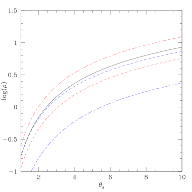
Figure 1: The ratio $\rho$ of cosmic variance over the noise due to the intrinsic ellipticity dispersion, from eq.(29), for the aperture-mass $M_{\rm ap}$. We show the results obtained for different surveys: “Wide” (solid line), “Wide+” (lower dashed line), “Wide-” (upper dot-dashed line), “Wide$>$” (upper dashed line) and “Wide$<$” (lower dot-dashed line).

We plot in Fig. 1 the ratio $\rho$ which measures the contribution to the noise from the “cosmic variance” relative to the effect associated with the intrinsic ellipticity dispersion, from eq.(29), for the aperture-mass $M_{\rm ap}$. Of course, we can check that $\rho$ increases with the radius $\theta_{s}$ of the filter (i.e. with the number $N$ of galaxies within the circular field of radius $\theta_{s}$). Thus, beyond a few arc-minutes the noise is dominated by the “cosmic variance”. For the same reason, as compared with the fiducial “Wide” survey (solid line), $\rho$ is larger for the “Wide-” survey (upper dot-dashed line), which is narrower but deeper, and smaller for the “Wide+” survey (lower dashed line). On the other hand, we can see that $\rho$ is much smaller for the low-$z$ subsample “Wide$<$” (lower dot-dashed line), which contains fewer galaxies and has a lower variance $\langle M_{\rm ap}^{2}\rangle$, while it is almost unchanged for the high-$z$ subsample “Wide$>$” (upper dashed line) which has also twice fewer galaxies but a larger variance $\langle M_{\rm ap}^{2}\rangle$. As seen in section 3.3, it will imply that although the skewness of the aperture-mass is smaller for the high-$z$ subsample (and more difficult to measure) the deviations of the pdf ${\cal P}(M)$ from the Gaussian are easier to measure. The ratio $\rho$ obtained for the shear components shows similar behaviours.

3.1 A specific case study: Wide SNAP survey

We first consider the case of the Wide SNAP survey, the properties of which are given in Table 1. We shall investigate the sensitivity to the survey parameters in next sections.

3.1.1 Variance

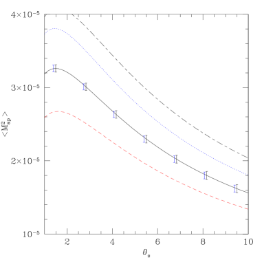
Figure 2: The variance $\langle M_{\rm ap}^{2}\rangle$ of the aperture-mass (solid curve). The largest error bars show the $1-\sigma$ dispersion $\sigma({\cal M}_{2})$ from eq.(47) and eq.(50). The smaller error bars which are slightly shifted to the left show the dispersion obtained by neglecting non-Gaussian contributions (i.e. $\langle M_{\rm ap}^{4}\rangle_{c}=0$ in eq.(47)). We also show the effect of a $10\%$ increase of $\Omega_{\rm m}$ (from $\Omega_{\rm m}=0.3$ up to $\Omega_{\rm m}=0.33$, central dotted curve), of a $10\%$ increase of the normalization $\sigma_{8}$ of the density power-spectrum (from $\sigma_{8}=0.88$ up to $\sigma_{8}=0.97$, upper dot-dashed curve), and of a $10\%$ decrease of the characteristic redshift $z_{0}$ (eq.(71)) of the survey (from $z_{0}=1.13$ down to $z_{0}=1.02$, lower dashed curve).

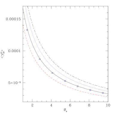
Figure 3: The variance $\langle\gamma_{i{\rm s}}^{2}\rangle$ of the smoothed shear component $\gamma_{i{\rm s}}$ (solid curve). The largest error bars show the $1-\sigma$ dispersion $\sigma({\cal M}_{2})$ from eq.(53) and eq.(52). The smaller error bars which are slightly shifted to the left show the dispersion obtained by neglecting non-Gaussian contributions (i.e. $\langle\gamma_{i{\rm s}}^{4}\rangle_{c}=0$ in eq.(53)). We also show the effect of a $10\%$ increase of $\Omega_{\rm m}$ (from $\Omega_{\rm m}=0.3$ up to $\Omega_{\rm m}=0.33$, central dotted curve), of a $10\%$ increase of the normalization $\sigma_{8}$ of the density power-spectrum (from $\sigma_{8}=0.88$ up to $\sigma_{8}=0.97$, upper dot-dashed curve), and of a $10\%$ decrease of the characteristic redshift $z_{0}$ (eq.(71)) of the survey (from $z_{0}=1.13$ down to $z_{0}=1.02$, lower dashed curve).

We show in Figs. 2-3 the variance of the aperture-mass $\langle M_{\rm ap}^{2}\rangle$ and of the smoothed shear component $\langle\gamma_{i{\rm s}}^{2}\rangle$ for the wide SNAP survey. As recalled above, this second-order moment is smaller for the aperture-mass $M_{\rm ap}$ which removes the contribution of long-wavelength density fluctuations to weak-lensing. Moreover, it bends down for small angular scales $\theta_{s}\la 1^{\prime}$ since in this regime the projected density $\kappa({\vec{\vartheta}})$ shows more power at larger scales (i.e. the non-linear density power-spectrum $P(k)$ grows more slowly than $k^{-2}$ at high $k$). We also display the $1-\sigma$ dispersion $\sigma({\cal M}_{2})$ from eq.(47) and eq.(50) (largest error bars in the figures). The smaller error bars which are slightly shifted to the left show the dispersion obtained by neglecting non-Gaussian contributions (i.e. $\langle M_{\rm ap}^{4}\rangle_{c}=0$ in eq.(47)). Thus, we can see that neglecting non-Gaussianities slightly underestimates the dispersion of the measurements but the difference with the full calculation is rather small. The relative size of the error bars is somewhat larger for the aperture-mass than for the shear because of the larger value of $\rho$. However, in both cases we can see that the wide survey of the SNAP mission should measure the variance of these weak-lensing observables up to a very good accuracy. We must point out, though, that this study does not take into account the possible systematic effects which might dominate the inaccuracy of the measures.

We also display the results obtained with a $10\%$ increase of $\Omega_{\rm m}$ (from $\Omega_{\rm m}=0.3$ up to $\Omega_{\rm m}=0.33$, central dotted curve), or a $10\%$ increase of the normalization $\sigma_{8}$ of the density power-spectrum (from $\sigma_{8}=0.88$ up to $\sigma_{8}=0.97$, upper dot-dashed curve), or a $10\%$ decrease of the characteristic redshift $z_{0}$ (eq.(71)) of the survey (from $z_{0}=1.13$ down to $z_{0}=1.02$, lower dashed curve). As is well-known and can be checked in Figs. 2-3, the amplitude of gravitational lensing distortions increases with $\Omega_{\rm m}$ and the matter density (see eq.(1)), with the amplitude $\sigma_{8}$ of the density fluctuations (see eq.(1)) and with the redshift $z_{0}$ as the line-of-sight is more extended. As seen in the figures, there is a clear degeneracy between these parameters. On the other hand, assuming other parameters are known we see that $\Omega_{\rm m}$ can be determined down to a few percents or to the relative accuracy of the redshift distribution and half the relative accuracy of $\sigma_{8}$.

Here we must note that the different points in Figs. 2-3 are not fully independent since different wavelengths of the underlying density field are somewhat correlated. In order to combine various angular scales to obtain an overall error-bar on a few cosmological parameters it is convenient to adopt a Fisher matrix approach (e.g., Hu & Tegmark 1999). However, we shall not investigate this traditional approach here, as it has already been studied in the literature.

3.1.2 Non-Gaussianities

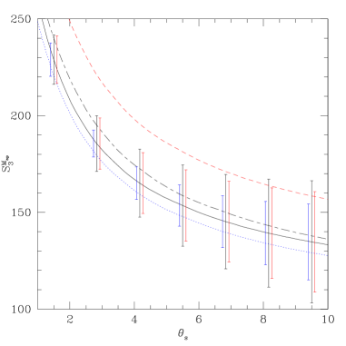
Figure 4: The skewness $S_{3}^{M_{\rm ap}}=\langle M_{\rm ap}^{3}\rangle/\langle M_{\rm ap}^{2}\rangle^{2}$ of the aperture-mass (solid curve). The central error bars show the $1-\sigma$ dispersion $\sigma({\cal S}_{3})$ from eq.(51). The smaller error bars which are slightly shifted to the left show the dispersion obtained by neglecting non-Gaussian contributions (i.e. $\langle M_{\rm ap}^{6}\rangle_{c}=\langle M_{\rm ap}^{4}\rangle_{c}=\langle M_{\rm ap}^{3}\rangle_{c}=0$ in eq.(48)). The smaller error bars which are slightly shifted to the right show the dispersion obtained from the estimator ${\cal S}_{3}^{H}$ in eq.(63). We also show the effect of a $10\%$ increase of $\Omega_{\rm m}$ (lower dotted curve), of a $10\%$ increase of $\sigma_{8}$ (central dot-dashed curve) and of a $10\%$ decrease of the redshift $z_{0}$ (upper dashed curve).

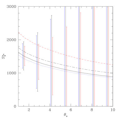
Figure 5: The kurtosis $S_{4}^{\gamma_{i{\rm s}}}=\langle\gamma_{i{\rm s}}^{4}\rangle_{c}/\langle\gamma_{i{\rm s}}^{2}\rangle^{3}$ of the smoothed shear component. The central error bars show the $1-\sigma$ dispersion $\sigma({\cal S}_{4})$ from eq.(56). The smaller error bars which are slightly shifted to the left show the dispersion obtained by neglecting non-Gaussian contributions (i.e. $\langle\gamma_{i{\rm s}}^{8}\rangle_{c}=\langle\gamma_{i{\rm s}}^{6}\rangle_{c}=\langle\gamma_{i{\rm s}}^{4}\rangle_{c}=0$ in eq.(54)). The smaller error bars which are slightly shifted to the right show the dispersion obtained from the estimator ${\cal S}_{4}^{H}$ in eq.(67). We also show the effect of a $10\%$ increase of $\Omega_{\rm m}$ (lower dotted curve), of a $10\%$ increase of $\sigma_{8}$ (central dot-dashed curve) and of a $10\%$ decrease of the redshift $z_{0}$ (upper dashed curve).

Next, we display in Figs. 4-5 the skewness $S_{3}^{M_{\rm ap}}$ of the aperture-mass and the kurtosis $S_{4}^{\gamma_{i{\rm s}}}$ of the shear component. These quantities provide a measure of the departure from Gaussianity of the underlying matter density field. They can also be used to break the degeneracy between the normalization of the density power-spectrum and the cosmological parameters (Bernardeau et al.1997). We can check that the error bars increase very fast with the order of the statistics. In particular, it is clear that the dispersion is dominated by the error bars associated with higher-order moments and we can neglect the dispersion due to the denominators $\langle M_{\rm ap}^{2}\rangle^{2}$ and $\langle\gamma_{i{\rm s}}^{2}\rangle^{3}$ which enter the definition of the skewness and kurtosis. The central error bars in the figures show the $1-\sigma$ dispersion $\sigma({\cal S}_{p})$ from eqs.(51),(56). It is much larger for the shear kurtosis, which is a higher-order statistics, than for the aperture-mass skewness. In particular, while the detection of non-Gaussianities from the aperture-mass should be clear up to $10^{\prime}$ and even somewhat beyond, it should become rather difficult from the shear component for angular scales $\theta_{s}\ga 6^{\prime}$. The smaller error bars which are slightly shifted to the left show the dispersion obtained by neglecting non-Gaussian contributions. Thus, neglecting non-Gaussianities again leads to an underestimate of the dispersion of the measures, but the effect remains small. On the other hand, the smaller error bars which are slightly shifted to the right show the dispersion obtained from the estimators ${\cal S}_{p}^{H}$ in eqs.(63),(67). As seen in section 2.4, these estimators which directly measure the cumulants always give a smaller dispersion than the estimators $M_{p}$ which measure the moments. We can see in Figs. 4-5 that the improvement is rather small for the skewness of the aperture-mass but it is already significant for the kurtosis of the shear. Therefore, these estimators should prove useful to extract quantitative informations from future weak-lensing surveys.

As for the variance, we also display the results obtained with a $10\%$ increase of $\Omega_{\rm m}$ (lower dotted curve), or a $10\%$ increase of $\sigma_{8}$ (central dot-dashed curve), or a $10\%$ decrease of the redshift $z_{0}$ (upper dashed curve). The skewness and the kurtosis show a modest dependence on the cosmological parameter (roughly of the same order: $8\%$) and they decrease for larger $\Omega_{\rm m}$. This can be understood from the factor $\Omega_{\rm m}$ which appears in eq.(1). They show a somewhat stronger dependence on $\sigma_{8}$ and they actually increase with $\sigma_{8}$ (so that $\Omega_{\rm m}$ and $\sigma_{8}$ have opposite effects on the skewness and the kurtosis while they acted in the same direction for the variance). This reflects the fact that a higher $\sigma_{8}$ implies a matter density field which is deeper in the non-linear regime and further away from the Gaussian. On the other hand, the skewness and the kurtosis show a strong variation with the redshift ($\sim 17\%$ and $\sim 40\%$) and they increase for a smaller source redshift. This can be understood from the fact that a larger source redshift means a longer line-of-sight (whence the pdf becomes closer to a Gaussian as we add the lensing contributions from successive mass sheets, following the central limit theorem) and a matter density field which is closer to Gaussian. Note that because the sensitivity onto $z_{0}$ and $\Omega_{\rm m}$ is different between the second and higher-order moments, they can be used to constrain both quantities and to remove the degeneracy between $z_{0}$ and $\Omega_{\rm m}$ which appeared in the variance. On the other hand, assuming that the redshift distribution is well known, higher order moments can also be used to break the degeneracy between the normalization $\sigma_{8}$ of the power-spectrum and the cosmological parameter $\Omega_{\rm m}$, as seen from the figures (also Bernardeau et al.1997). However, our results show that the error bar on the measure of $\Omega_{\rm m}$ cannot be smaller than twice the error bar on the redshift distribution.

3.1.3 Probability distribution functions

Aperture-mass $M_{\rm ap}$

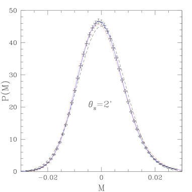
Figure 6: The pdf ${\cal P}(M)$ from eq.(32) for the estimator $M$ associated with the aperture-mass $M_{\rm ap}$ as defined in eq.(26). Note that the Gaussian noise introduced by intrinsic ellipticities makes ${\cal P}(M)$ closer to the Gaussian than the actual pdf ${\cal P}(M_{\rm ap})$ which only takes into account gravitational lensing. The solid line shows the theoretical prediction (32), the dashed line is the Gaussian and the dotted line is the Edgeworth expansion (57) up to the first non-Gaussian term (the skewness). The error bars show the $1-\sigma$ dispersion $\sigma(P_{k})$ from eq.(37).

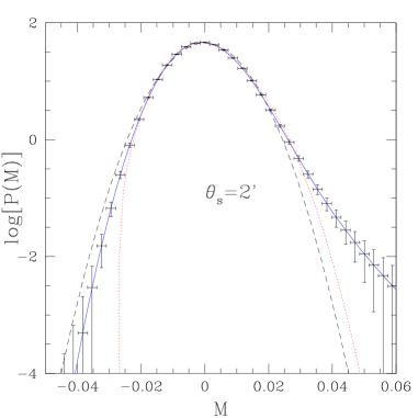
Figure 7: The logarithm $\log({\cal P}(M))$ of the pdf shown in Fig. 6. The error bars correspond to $\log({\cal P}(M)\pm\sigma)$, from eq.(37).

Finally, we show in Figs. 6-7 the pdf ${\cal P}(M)$ obtained for the estimator $M$ defined in eq.(26). As seen in section 2.2, these pdfs are actually the convolution of the pdf ${\cal P}(M_{\rm ap})$ (which measures gravitational lensing) by the Gaussian of variance $\sigma_{*}^{2}$ associated with the noise due to the galaxy intrinsic ellipticity dispersion and to the detector white noise. This convolution makes the final pdf ${\cal P}(M)$ closer to Gaussian than the actual ${\cal P}(M_{\rm ap})$. We consider the angular scale $\theta_{s}=2^{\prime}$ and we display the theoretical prediction (32) (solid line), the Gaussian (dashed line) and the Edgeworth expansion (57) up to the first non-Gaussian term (i.e. the skewness) (dotted line). We also show the $1-\sigma$ error bars obtained from eq.(37). We chose for the width $\Delta$ of the intervals the values $\Delta=\langle M^{2}\rangle^{1/2}/8$ in Fig. 6 and $\Delta=\langle M^{2}\rangle^{1/2}/3$ in Fig. 7. We can see from Fig. 6 that it should be possible to measure the departure from the Gaussian near the peak of ${\cal P}(M)$, which is slightly higher and shifted towards negative $M$. This also translates the asymmetry of ${\cal P}(M_{\rm ap})$. On the other hand, from Fig. 7 it appears that the far positive tail of ${\cal P}(M)$, for $M\simeq 0.05$, should also provide a means to detect such non-Gaussianities. One should also be able to extract some useful information from the negative tail at $M\simeq-0.03$. Note that it should be possible to distinguish ${\cal P}(M)$ from both the Gaussian and the Edgeworth expansion. This means that one has access to more information than is encoded in the variance and the skewness. Thus, it would be interesting to check in future surveys that these three domains of ${\cal P}(M)$ show the expected behaviour which characterizes the non-Gaussianities brought by non-linear gravitational clustering. From another point of view, the expected shape of ${\cal P}(M)$ due to gravitational lensing might be useful in order to discriminate this signal from possible non-Gaussianities induced by the detector (which might contaminate the measure of the skewness).

Smoothed shear component $\gamma_{i{\rm s}}$

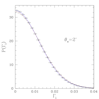
Figure 8: The pdf ${\cal P}(\Gamma_{i})$ from eq.(32) for the estimator $\Gamma_{i}$ associated with the smoothed shear component $\gamma_{i{\rm s}}$ as defined in eq.(39). Note that the Gaussian noise introduced by intrinsic ellipticities makes ${\cal P}(\Gamma_{i})$ closer to the Gaussian than the actual pdf ${\cal P}(\gamma_{i{\rm s}})$ which only takes into account gravitational lensing. The solid line shows the theoretical prediction (32), the dashed line is the Gaussian and the dotted line is the Edgeworth expansion (57) up to the first non-Gaussian term (the kurtosis). The error bars show the $1-\sigma$ dispersion $\sigma(P_{k})$ from eq.(43).

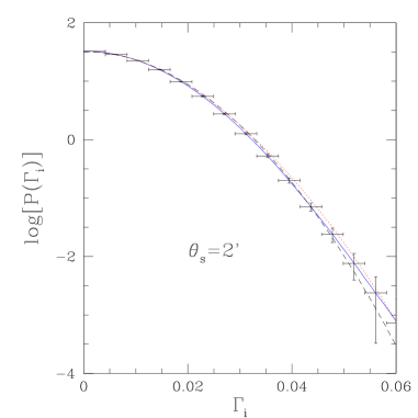
Figure 9: The logarithm $\log({\cal P}(\Gamma_{i}))$ of the pdf shown in Fig. 8. The error bars correspond to $\log({\cal P}(\Gamma_{i})\pm\sigma)$, from eq.(43).

We show in Figs. 8-9 the pdf ${\cal P}(\Gamma_{i})$ obtained for the estimator $\Gamma_{i}$ defined in eq.(39). As for the aperture-mass, this is actually the convolution of ${\cal P}(\gamma_{i{\rm s}})$ by a Gaussian of variance $\sigma_{*}^{2}$, which models the noise due to galaxy intrinsic ellipticities and detector white noise. We again display the theoretical prediction (32) (solid line), the Gaussian (dashed line) and the Edgeworth expansion (57) up to the first non-Gaussian term (i.e. the kurtosis). The $1-\sigma$ error bars are obtained from eq.(43) with $\Delta=\langle\Gamma_{i}^{2}\rangle^{1/2}/8$ in Fig. 8 and $\Delta=\langle\Gamma_{i}^{2}\rangle^{1/2}/3$ in Fig. 9. We see from Fig. 8 that it should again be possible to measure the deviations from Gaussianity near the peak of ${\cal P}(\Gamma_{i})$ ($\Gamma_{i}\simeq 0$), which is slightly higher than for a Gaussian. The non-Gaussianity might also be measured from the near tail of ${\cal P}(\Gamma_{i})$, at $\Gamma_{i}\simeq 0.02$. As for the aperture-mass, measuring the pdf ${\cal P}(\Gamma_{i})$ in two different ranges provides useful information since it can be used to check the shape of the non-Gaussianities expected from non-linear gravitational clustering, or to discriminate the signal from spurious non-Gaussianities introduced by the detector. Note indeed that one should be able to distinguish ${\cal P}(\Gamma_{i})$ from both the Gaussian and the Edgeworth expansion. On the other hand, we see from Fig. 9 that the far tail of the pdf ($\Gamma_{i}\ga 0.04$) is too noisy to give useful constraint on non-Gaussianities, contrary to the aperture-mass.

3.2 Survey strategy: Width vs. Depth

We have seen in the previous sections that the nominal Wide SNAP survey should yield useful information about the amplitude and the non-Gaussianities of the matter density fluctuations. We now study the dependence of these results on the survey properties. Thus, following Refregier et al. (2004), we compare this Wide SNAP survey with the Deep survey realized by the same mission (designed for the search for Type Ia supernovae) and with two hypothetical surveys, labeled “Wide+” and “Wide-” in Table 1, with the same observing time (5 months) and a survey area $A$ which is doubled or halved (implying a smaller or larger depth at fixed observing time).

3.2.1 Variance

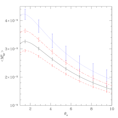
Figure 10: The variance $\langle M_{\rm ap}^{2}\rangle$ of the aperture-mass for the Wide survey (solid line), the Deep survey (dotted line), the “Wide+” survey (lower dashed line) and the “Wide-” survey (upper dot-dashed line). The error bars show the $1-\sigma$ dispersion $\sigma({\cal M}_{2})$ from eq.(47) and eq.(50).

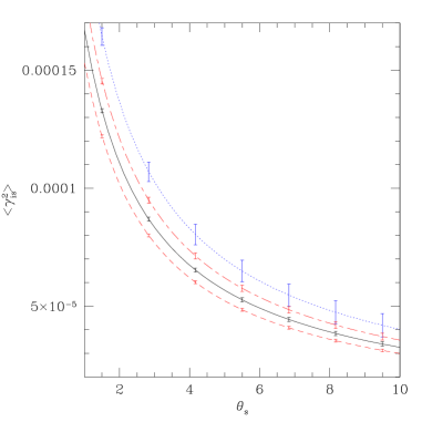
Figure 11: The variance $\langle\gamma_{i{\rm s}}^{2}\rangle$ of the smoothed shear component $\gamma_{i{\rm s}}$ for the Wide survey (solid line), the Deep survey (dotted line), the “Wide+” survey (lower dashed line) and the “Wide-” survey (upper dot-dashed line). The error bars show the $1-\sigma$ dispersion $\sigma({\cal M}_{2})$ from eq.(47) and eq.(50).

We show in Figs. 10-11 the variance of the aperture-mass $\langle M_{\rm ap}^{2}\rangle$ and of the smoothed shear component $\langle\gamma_{i{\rm s}}^{2}\rangle$ for these four surveys: “Wide” (solid line, as in section 3.1.1), “Deep” (dotted line), “Wide+” (dashed line) and “Wide-” (dot-dashed line). Of course, the variance is larger for the Deep survey since the redshift distribution is broader. However, its error bars are larger because the total survey area is much smaller. In agreement with Refregier et al. (2004), we find that the widest survey “Wide+” yields slightly smaller error bars than the nominal survey “Wide” (or the narrower survey “Wide-”). Hence a wider and shallower survey is slightly more efficient but the difference is probably too small to have any impact on observational strategies.

3.2.2 Non-Gaussianities

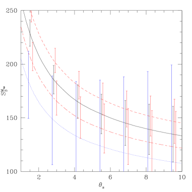
Figure 12: The skewness $S_{3}^{M_{\rm ap}}$ of the aperture-mass for the Wide survey (solid line), the Deep survey (dotted line), the “Wide+” survey (upper dashed line) and the “Wide-” survey (lower dot-dashed line). The error bars show the dispersion obtained from the estimator ${\cal S}_{3}^{H}$ in eq.(63).

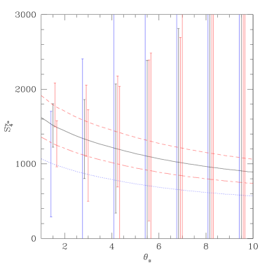
Figure 13: The kurtosis $S_{4}^{\gamma_{i{\rm s}}}$ of the smoothed shear component for the Wide survey (solid line), the Deep survey (dotted line), the “Wide+” survey (upper dashed line) and the “Wide-” survey (lower dot-dashed line). The error bars show the dispersion obtained from the estimator ${\cal S}_{4}^{H}$ in eq.(67).

Next, we display in Figs. 12-13 the skewness $S_{3}^{M_{\rm ap}}$ of the aperture-mass and the kurtosis $S_{4}^{\gamma_{i{\rm s}}}$ of the shear component for the four surveys. The error bars correspond to the estimators $H_{p}$ which show less scatter than $M_{p}$. The skewness and the kurtosis are smaller for the “Deep” and “Wide-” surveys which have a redshift distribution of sources which is more heavily weighted by high redshifts. As for the variance, the “Wide+” survey yields the best results, since it exhibits larger non-Gaussianities and smaller error bars. Thus, it enables one to detect non-Gaussianities up to slightly larger angular scales than the nominal “Wide” survey would allow.

3.3 Survey strategy: Redshift binning

In the previous sections, we have described how the quality of the information obtained from weak lensing measures depend on the survey properties. However, once a specific survey is realized one still has the possibility to analyze the data in different ways, for instance by subdividing the galaxy sample into several redshifts bins. This can be conveniently done by using photometric redshifts. To investigate this issue, we describe in this section the results which can be obtained by dividing the Wide SNAP survey, given in Table 1, into two redshifts bins: $z_{s}>z_{*}$ (which we denote by “Wide$>$”) and $z<z_{*}$ (which we refer to as “Wide$<$”). We choose $z_{*}=1.23$, which corresponds roughly to the separation provided by the SNAP filters and which splits the Wide SNAP survey into two samples with the same number of galaxies (hence $n_{g}=50$ arcmin^-2).

3.3.1 Variance

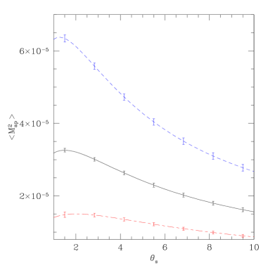
Figure 14: The variance $\langle M_{\rm ap}^{2}\rangle$ of the aperture-mass for the full Wide survey (solid line), the high-$z$ “Wide$>$” sample (upper dashed line) and the low-$z$ “Wide$<$” sample (lower dot-dashed line). The error bars show the $1-\sigma$ dispersion $\sigma({\cal M}_{2})$ from eq.(47) and eq.(50).

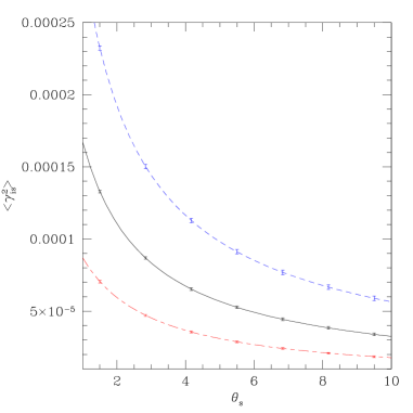
Figure 15: The variance $\langle\gamma_{i{\rm s}}^{2}\rangle$ of the smoothed shear component $\gamma_{i{\rm s}}$ for the full Wide survey (solid line), the high-$z$ “Wide$>$” sample (upper dashed line) and the low-$z$ “Wide$<$” sample (lower dot-dashed line). The error bars show the $1-\sigma$ dispersion $\sigma({\cal M}_{2})$ from eq.(47) and eq.(50).

We show in Figs. 14-15 the variance of the aperture-mass and of the smoothed shear component for the three samples: the full Wide SNAP survey (solid line), the high-$z$ “Wide$>$” sample (upper dashed line) and the low-$z$ “Wide$<$” sample (lower dot-dashed line). Of course, we find that the variance is larger for the high-$z$ sample since the amplitude of weak lensing distortions increases with the redshift of the source (and the length of the line-of-sight). Note that the error bars are quite small for all three samples therefore it is interesting to divide the survey into several redshift bins which allow one to check the evolution with time of the matter power-spectrum. This also provides stronger constraints on cosmological parameters (and possibly on the equation of state of the dark energy, which we shall not investigate here).

We must note that the different curves in Figs. 14-15 show some correlation since the lines of sight to distant sources located in different redshift bins probe the same density fluctuations at low $z$. Again it can be convenient to use a Fisher matrix approach to combine these various redshifts. We shall study the cross-correlations between different redshift subsamples in a future paper (Munshi & Valageas 2004).

3.3.2 Non-Gaussianities

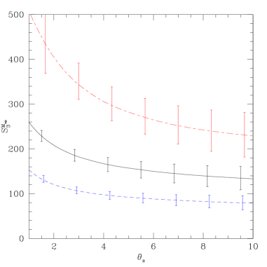
Figure 16: The skewness $S_{3}^{M_{\rm ap}}$ of the aperture-mass for the full Wide SNAP survey (solid line), the high-$z$ “Wide$>$” sample (lower dashed line) and the low-$z$ “Wide$<$” sample (upper dot-dashed line). The error bars show the dispersion obtained from the estimator ${\cal S}_{3}^{H}$ in eq.(63).

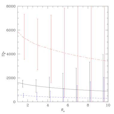
Figure 17: The kurtosis $S_{4}^{\gamma_{i{\rm s}}}$ of the smoothed shear component for the full Wide survey (solid line), the high-$z$ “Wide$>$” sample (lower dashed line) and the low-$z$ “Wide$<$” sample (upper dot-dashed line). The error bars show the dispersion obtained from the estimator ${\cal S}_{4}^{H}$ in eq.(67).

Next, we show in Figs. 16-17 the skewness $S_{3}^{M_{\rm ap}}$ of the aperture-mass and the kurtosis $S_{4}^{\gamma_{i{\rm s}}}$ of the smoothed shear component for the three samples. The parameters $S_{p}$ are smaller for the high-$z$ sample (lower dashed line) which involves the convolution of the weak lensing effects arising from many successive mass sheets (which makes the signal closer to Gaussian, following the central limit theorem) and which probes a density field which is closer to the linear Gaussian regime. In the case of the aperture-mass, all three samples allow a clear detection of non-Gaussianity and a rather precise measure of $S_{3}^{M_{\rm ap}}$. As for the variance, it will be interesting to perform such a redshift binning of the data in order to check the evolution with redshift of $S_{3}^{M_{\rm ap}}$. This should strengthen the constraints obtained from observations. Moreover, it could be useful in order to discriminate the non-Gaussianities due to the non-linear gravitational dynamics from those associated with the noise which might be non-Gaussian (whether it comes from the galaxy intrinsic ellipticities or the detector itself). In the case of the shear component the three samples enable one to detect non-Gaussianity at small angular scales $\theta_{s}\la 4^{\prime}$ while the low-$z$ sample allows one to go up to slightly larger angles, $\theta_{s}\la 7^{\prime}$, because it yields a kurtosis which is much larger. Note that in both cases, the skewness or the kurtosis shows a strong variation with the redshift binning, which should easily be detected.

3.3.3 Probability distribution functions

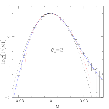
Figure 18: The logarithm $\log({\cal P}(M))$ of the pdf ${\cal P}(M)$ from eq.(32) for the high-$z$ sample “Wide$>$”, for the estimator $M$ associated with the aperture-mass $M_{\rm ap}$ as defined in eq.(26). The solid line shows the theoretical prediction (32), the dashed line is the Gaussian and the dotted line is the Edgeworth expansion (57) up to the first non-Gaussian term (the skewness). The error bars correspond to $\log({\cal P}(M)\pm\sigma)$, from eq.(37).

Finally, we display in Fig. 18 the pdf ${\cal P}(M)$ obtained for the estimator $M$ associated with the aperture-mass $M_{\rm ap}$ for the high-$z$ sample “Wide$>$”. Indeed, although the skewness $S_{3}^{M_{\rm ap}}$ is larger for the low-$z$ sample, its pdf ${\cal P}(M)$ is closer to Gaussian because the variance $\langle M_{\rm ap}^{2}\rangle$ is smaller so that the influence of the intrinsic galaxy ellipticities is larger and this turns out to be the main factor. Therefore, we find that for the low-$z$ sample the pdf ${\cal P}(M)$ cannot be easily distinguished from the Gaussian. By contrast, as seen in Fig. 18 the high-$z$ sample still allows a clear detection of non-Gaussianity. In fact, as for the full sample studied in section 3.1.3, the tails of the distribution enable one to distinguish ${\cal P}(M)$ from both the Gaussian and the Edgeworth expansion. This should again prove useful. On the other hand, the pdf ${\cal P}(\Gamma_{i})$ cannot be distinguished from the Gaussian, except near its peak for the full sample.

4 Discussion

Weak lensing surveys are already being used to constrain allowed regions of cosmological parameter space. Future surveys such as SNAP will provide a better opportunity by covering a large fraction of the sky. While there has been a tremendous progress in understanding the effect of cosmological parameters on weak lensing statistics, a complete analysis of realistic noise contribution for various survey strategies is still lacking.

In this paper we have mainly focused on realistic surveys such as SNAP to compute the estimator induced variance due to contributions from the finite catalogue size and the intrinsic ellipticity distribution of galaxies. Although Poisson effects (due to the discrete distribution of galaxies) are quite small for such surveys because of the high surface density of galaxies $n_{g}$, the other contributions can play a dominant role. We study both the aperture-mass $M_{\rm ap}$ and the smoothed shear components $\gamma_{i{\rm s}}$, which can be more easily recovered from actual surveys than the smoothed convergence $\kappa_{\rm s}$. Extending earlier works which focused on the lower order cumulants, we present a unified approach in order to handle both cumulants and the full pdfs of these objects.

In agreement with previous works (Refregier et al. 2004), we find that surveys like the SNAP mission can measure the variance of both $M_{\rm ap}$ and $\gamma_{i{\rm s}}$ up to a very good accuracy (a few percent) for the entire range of angular scales $1^{\prime}<\theta_{s}<10^{\prime}$ that we have studied. This should yield strong constraints on the cosmological parameters (e.g., a measure of $\Omega_{\rm m}$ to a few percent if all other parameters are known). However, there is a well-known degeneracy between $\Omega_{\rm m}$ and $\sigma_{8}$. In addition, we find that $\Omega_{\rm m}$ cannot be measured to better than the relative accuracy of the redshift distribution, which might be a significant limitation.

As usual, the degeneracy between several cosmological parameters can be removed by measuring higher-order moments. We find that the skewness $S_{3}^{M_{\rm ap}}$ of the aperture-mass should be easily detected and measured up to a $10\%$ accuracy over $1^{\prime}<\theta_{s}<10^{\prime}$. By contrast, the shear kurtosis $S_{4}^{\gamma_{i{\rm s}}}$ should be difficult to measure beyond $6^{\prime}$. Indeed, higher-order cumulants are increasingly difficult to measure from noisy data: their scatter grows with their order as a larger number of terms contributes to their dispersion which also involves all cumulants up to twice their order. Using a realistic model for the underlying matter density field, our computation of these error bars takes into account all these cumulants (that is we do not keep only the Gaussian terms or multiply this contribution by a fudge factor), which slightly increase the dispersion. On the other hand, we introduced a new class of estimators ${\cal H}_{p}$ designed to measure these low-order cumulants. We have shown that they yield a scatter which is always smaller than the one obtained by using the simple estimators ${\cal M}_{p}$ derived from the moments themselves (and are actually optimal among a one-parameter family of estimators for a Gaussian distribution). We find that the gain is rather small for the skewness $S_{3}^{M_{\rm ap}}$ but for the kurtosis $S_{4}^{\gamma_{i{\rm s}}}$ we get a significant reduction of the scatter. Since these estimators are no more difficult to use than the naive ${\cal M}_{p}$ estimators they should be preferred over the latter. The skewness or the kurtosis may be used to remove the degeneracy between $\Omega_{\rm m}$ and $\sigma_{8}$ so as to enable one to measure the cosmological parameters. However, we note that they are very sensitive to the redshift of the sources, so that the accuracy of $\Omega_{\rm m}$ cannot be smaller than twice the error bar on the redshift of the galaxy distribution. On the other hand, by binning the sample over redshift one might be able to discriminate the influence of the redshift.

In addition to the low-order moments we have also studied the full pdfs ${\cal P}(M)$ and ${\cal P}(\Gamma_{i})$, where $M$ (resp. $\Gamma_{i}$) is a biased estimator of the aperture-mass (resp. of the shear component). Here the intrinsic galaxy ellipticity distribution plays a key role as it makes $M$ and $\Gamma_{i}$ biased estimators and it makes the pdfs ${\cal P}(M)$ and ${\cal P}(\Gamma_{i})$ much closer to the Gaussian than the pdfs ${\cal P}(M_{\rm ap})$ and ${\cal P}(\gamma_{i{\rm s}})$. Note that the intrinsic galaxy ellipticity also contributed to the measure of the low-order cumulants but it was less of a problem because one can still build unbiased estimators of these low-order cumulants (by counting each galaxy only once, which also removes some contributions to their scatter). We find that the pdfs ${\cal P}(M)$ and ${\cal P}(\Gamma_{i})$ can be distinguished from a Gaussian through their shape near their maximum. Moreover, the negative and positive tails of the pdf ${\cal P}(M)$ associated with the aperture-mass can be discriminated from both the Gaussian and the Edgeworth expansion (using only the first non-Gaussian term defined by the skewness). This means that one can extract more information than is encoded in the first two low-order moments. Moreover, by measuring the pdf ${\cal P}(M)$ over these three domains one should be able to strengthen the constraints derived for the underlying matter density field and to discriminate possible non-Gaussianities induced by the detector. On the other hand, we find that the far tails of the symmetric pdf ${\cal P}(\Gamma_{i})$ associated with the shear component are too noisy to give useful constraints. A detailed $\chi^{2}$ analysis will be presented elsewhere for simulated observations.

Next, we have investigated whether the information obtained from observations could be improved by changing the survey strategy. Thus, we have compared the nominal wide SNAP survey with the “Deep” SNAP survey as well as with two hypothetical surveys with the same observing time as a the original survey but a different trade-off between area and depth. We focused on the first two low-order moments for the aperture-mass and the shear component. In agreement with Refregier et al. (2004) (who studied the lensing power-spectrum and the convergence skewness) we find that a wider and shallower survey is slightly more efficient.

Finally, we have studied the possibility to divide the wide SNAP survey into two redshift bins ($z<1.23$ and $z>1.23$). All three samples provide a very accurate measure of the variance of both the aperture-mass and the shear component. As noticed above, this should allow one the improve the constraints and to check the evolution with redshift of non-linear gravitational clustering. The skewness $S_{3}^{M_{\rm ap}}$ is also well measured in the three samples, while the kurtosis $S_{4}^{\gamma_{i{\rm s}}}$ is more easily obtained from the low-$z$ sample. This shows again the interest of such a redshift binning of the data. In addition, the high-$z$ sample again allows a good measure of the pdf ${\cal P}(M)$ associated with the aperture-mass, which can be distinguished from both the Gaussian and the Edgeworth expansion.

In this article we have mainly focused on errors associated with quantities derived from a specific redshift bin. We shall extend our studies to the cross correlations among various redshift bins in future works (Munshi & Valageas 2004). This can also be generalized to compute the cross correlations among various statistics derived from different surveys with non-identical scan strategies.

Throughout our studies we have ignored source clustering and the effect due to lens coupling. A detailed prediction of source clustering and lens coupling will require an accurate picture of how galaxy number densities are related to the underlying mass distribution. Some of these issues have been studied by Bernardeau (1997), Bernardeau et al. (1997) and Schneider et al. (1998) who found that such corrections are negligible at least in the quasi-linear regime. In the non-linear regime one might use numerical simulations in order to evaluate this affect, but this would again require a specific recipe for the correlation between galaxies and dark matter.

Another ingredient in our calculations has been the so called Born approximation. Its validity can only be checked numerically in the highly non-linear regime. Thus, the consistency of analytical results and numerous numerical simulations found in previous studies strongly suggests that this approximation remains accurate in the highly non-linear regime (see also Vale & White 2003).

In our studies we also assumed that the intrinsic ellipticities of different galaxies are uncorrelated (Heymans & Heavens 2003, Crittenden et al. 2001) (but of course we take into account its variance). Techniques to deal with such correlations have been studied in detail although the extent to which such correlations will affect weak lensing surveys remains somewhat uncertain. It is however generally believed that such effects will play a less important role as we increase the survey depth and we can reduce their role through acquisition of photometric redshift (Heymans & Heavens 2003).

Although almost all present studies assume these intrinsic ellipticities to be Gaussian random variables this might not be the case. Any signature of such non-Gaussianity if found by observational teams will have to be folded into analytical calculations. This can be performed in a straightforward way within our formalism. In this case, the measure of full pdfs like ${\cal P}(M)$ or ${\cal P}(\Gamma_{i})$ would be of great interest in order to disantengle the signal from the non-Gaussianities due to galaxy ellipticities (which might contaminate low-oder moments, especially if there are cross-correlations). However, if such intrinsic non-Gaussianities are too large they might dominate the signal and preclude an accurate measure of the non-Gaussianities due to the matter density field. In addition to the galaxy intrinsic ellipticities and to the finite size of the survey, another source of noise is given by the finite PSF effects (smear). It would be interesting to include this contribution in future studies.

References

- [1] Bacon D.J., Refregier A., Ellis R.S., 2000, MNRAS, 318, 625
- [2] Barber A. J., Munshi D., Valageas P., 2004, MNRAS, 347, 665
- [3] Bernardeau F., Kofman L., 1995, ApJ, 443, 479
- [4] Bernardeau F., Schaeffer R., 1992, A&A, 255, 1
- [5] Bernardeau F., Valageas P., 2000, A&A, 364, 1
- [6] Bernardeau F., Van Waerbeke L., Mellier Y., 1997, A&A, 322, 1
- [7] Couchman H. M. P., Barber A. J., Thomas P. A., 1999, MNRAS, 308, 180
- [8] Crittenden R.G., Natarajan P., Pen U., Theuns T., 2001, ApJ, 559, 552
- [9] Cooray A., Sheth R., 2002, Phys.Rept., 372 ,1
- [10] Fry J.N., 1984, ApJ, 279, 499
- [11] Heymans C., Heavens A., 2003, MNRAS, 339, 711
- [12] Hoekstra H., Yee H. K. C., Gladders M. D., 2002, ApJ, 577, 595
- [13] Hu W., Tegmark M., 1999, ApJ, 514, L65
- [14] Jain B., Seljak U., 1997, ApJ, 484, 560
- [15] Jain B., Seljak U., White S.D.M., 2000, ApJ, 530, 547
- [16] Jaroszynski M., Park C., Paczynski B., Gott J.R., 1990, ApJ, 365, 22
- [17] Kaiser N., 1992, ApJ, 388, 272
- [18] Kaiser N., Squires G., Fahlman G., Woods D., 1994, in: Durret F., Mazure A., Tran Thanh Van J. (eds.) Clusters of galaxies. Editions Frontieres
- [19] Kaiser N., 1998, ApJ, 498, 26
- [20] Munshi D., 2000, MNRAS, 318, 145
- [21] Munshi D., Jain B., 2000, MNRAS, 318, 109
- [22] Munshi D., Jain B., 2001, MNRAS, 322, 107
- [23] Munshi D., Coles P., 2003, MNRAS, 338, 846
- [24] Munshi D., Valageas P., 2004, astro-ph/0406081
- [25] Munshi D., Melott A.L., Coles P., 1999, MNRAS, 311, 149
- [26] Munshi D., Valageas P., Barber A. J., 2004, MNRAS, 350, 77
- [27] Peacock J.A., Dodds S.J., 1996, MNRAS, 280, L19
- [28] Peacock J.A., Smith R. E., 2000, MNRAS, 318, 1144
- [29] Refregier A. et al., 2004, AJ, 127, 3102
- [30] Schaeffer R., 1984, A&A, 134, L15
- [31] Schneider P., 1996, MNRAS, 283, 837
- [32] Schneider P., van Waerbeke L., Jain B., Kruse G., 1998, MNRAS, 296, 873
- [33] Schneider P., Weiss A., 1988, ApJ, 330,1
- [34] Szapudi I., Szalay A.S., 1993, ApJ, 408, 43
- [35] Szapudi I., Szalay A.S., 1997, ApJ, 481, L1
- [36] Takada M., Jain B., 2002, MNRAS, 337, 875
- [37] Takada M., Jain B., 2003a, MNRAS, 344, 857
- [38] Takada M., Jain B., 2003b, MNRAS, 346, 949
- [39] Valageas P., 2000a, A&A, 354, 767
- [40] Valageas P., 2000b, A&A, 356, 771
- [41] Valageas P., Barber A. J., Munshi D., 2004, MNRAS, 347, 652
- [42] Vale C., White M., 2003, ApJ, 592, 699
- [43] Van Waerbeke L., Bernardeau F., Mellier Y., 1999, A& A, 342, 15
- [44] Van Waerbeke L., Hamana T., Scoccimarro R., Colombi S., Bernardeau F., 2001, MNRAS, 322, 918
- [45] Van Waerbeke L., Mellier Y., Pelló R., Pen U.-L., McCracken H.J., Jain B., 2002, A&A, 393, 369
- [46] Villumsen J.V., 1996, MNRAS, 281, 369
- [47] Wambsganss J., Cen R., Ostriker J.P., 1998, ApJ, 494, 29
- [48] Zhang T.-J., Pen U.-L., Zhang P., Dubinski J., 2003, ApJ, 598, 818