Analysis of the Kamionkowski-Loeb method of reducing
cosmic variance with CMB polarizationls

Abstract

Part of the CMB polarization signal in the direction of galaxy clusters is produced by Thomson scattering of the CMB temperature quadrupole. In principle this allows measurement of the CMB power spectrum harmonic $C_{2}(z)$ with higher accuracy (at $z>0$) than the cosmic variance limit imposed by sample variance on one CMB sky. However the observed signals are statistically correlated if the comoving separation between the clusters is small enough. Thus one cannot reduce the sample variance by more than roughly the number of separate regions available which produce uncorrelated signals, as first pointed out by Kamionkowski and Loeb. In this paper we analyze in detail the procedure outlined by Kamionkowski and Loeb, computing the correlation of the polarization signals by considering the variation of the spherical harmonic expansion coefficients of the temperature anisotropy on our past light cone.

Given a hypothetical set of Stokes parameter measurements of the CMB polarization in the directions of galaxy clusters, distributed at random on a given redshift shell, we show how to construct an estimator of the angular power spectrum harmonic $C_{2}$ at that redshift. We then compare the variance of this estimator with the cosmic variance of the CMB multipole on our sky which probes the same scale. We find that in fact the cosmic variance is not reducible below the single sky CMB value using the cluster method. Thus this method is not likely to be of use for reconstruction of the primordial power spectrum. However the method does yield a measurement of $C_{2}$ as a function of redshift with increasing accuracy at higher redshift, and thus potentially a probe of the mechanism which may have suppressed the quadrupole.

We also examine to what extent the redshift dependence of $C_{2}$ can be used to probe the time changing potential anisotropy as the universe evolves into the vacuum dominated phase (the late-time integrated Sachs-Wolfe effect). We find that this effect is not observable in the time dependence of $C_{2}$ since it is swamped by cosmic variance, but there is an observable signature in the correlation functions of the Stokes parameters.

I Introduction

The CMB radiation incident on galaxy clusters has an intrinsic intensity quadrupole $Q_{2}$ created by inhomogeneity at the surface of last scattering. Thomson scattering of the CMB in a galaxy cluster with typical line of sight optical depth $\tau_{\rm C}$ generates polarization of order $Q_{2}\tau_{\rm C}$. Thus a measurement of this polarization signal would allow an estimate of the CMB quadrupole at non-zero redshift. This is of interest because it would potentially allow us to get around the restriction of cosmic variance. To elaborate, at $z=0$ we only have one CMB sky to observe, with $(2l+1)$ independent real data points for each spherical harmonic mode of the CMB on our sky, to compare with the ensemble average prediction of the variance. There is thus an intrinsic fractional sample variance of the harmonic $C_{l}$ of $2/(2l+1)$ (see section §II), which severely limits comparison with the ensemble averaged theory at low $l$. This restriction limits the accuracy of measurements of the primordial power spectrum on the largest scales. The theoretical predictions thus obtained for the CMB power spectra are fundamentally limited by this sample variance, commonly termed the cosmic variance.

Thomson scattering of the $l=2$ part of the CMB anisotropy in a cluster generates a secondary polarization anisotropy which depends on the spherical harmonic components $a_{2m}$ as seen by a (hypothetical) observer at the cluster. Since this polarization signal produced by a cluster is sensitive to the density perturbations on a last scattering surface different to our own, this in principle allows one to make more accurate comparison to the theoretical predictions for CMB angular power spectra at low $l$ than allowed by the cosmic variance limit. However the observed signals are correlated if the comoving separation between the clusters is small, and many strongly correlated signals are no more useful for reducing the sample variance than one signal. The variance in the estimated quadrupole can be reduced by roughly the number of regions available which produce uncorrelated signals.

This method of using the CMB polarization signal produced by galaxy clusters to get around cosmic variance limits was first pointed out by Kamionkowski and Loeb Kamionkowski:1997na (we usually refer to it as the “cluster method” in what follows). However Kamionkowski and Loeb did not actually compute the correlation of the cluster signals in a particular cosmological model in their paper, and did not therefore demonstrate explicitly that the cosmic variance is reduced with a given set of clusters, nor did they develop any formalism for converting measurements of the Stokes parameters of the CMB to statistical estimators which get around cosmic variance. In 2003PhRvD..67f3505C , estimators of $C_{2}(\tau)$ were constructed (taking into account the kinematic SZ contamination of the polarization signal also), but the effect of statistical variation in the polarization signal on the estimator variance was not included. This variation was considered by 2000PhRvD..62l3004S , but they computed the variation of the quadrupole as an expansion in small cluster separations, and their analysis is not applicable to a general set of clusters in arbitrary locations. In this paper we compute the correlation of the cluster signals in the case of an idealized set of measurements from clusters distributed in random directions on a given redshift shell. We describe an explicit procedure for carrying out the program outlined in Kamionkowski:1997na , and study how the correlations die off as clusters of increasingly high redshift are used. Information about the correlation of the polarization signals is contained in the generalized correlation functions of the CMB temperature anisotropy coefficients, $\langle a_{lm}(\mbox{\boldmath$x$},\tau)a^{*}_{l^{\prime}m^{\prime}}(\mbox{\boldmath$x$}^{\prime},\tau^{\prime})\rangle$, which contain all of the statistical information (assuming Gaussianity) about the variation of the $a_{lm}$ coefficients as the observation point and associated last scattering surface change. With these functions, we can derive an estimator for $C_{2}(z)$ in terms of Stokes parameters, and find its variance.

We should clarify exactly what we mean by reducing cosmic variance. It is true that the polarization signals provide an estimator $\hat{C}_{2}(\tau)$ of the remote quadrupole at a given redshift which has a smaller fractional cosmic variance than the local quadrupole. However, this is not the most useful comparison, since this estimator probes smaller physical scales than the local quadrupole. Cosmologists already have estimators of the power on these scales, namely the WMAP angular power spectrum harmonics $C_{l}$ with $l>2$. So the interesting question to ask is whether $\hat{C}_{2}(\tau)$ has smaller cosmic variance than the CMB multipole on our sky that probes the same physical scale. This determines whether or not the cluster technique is capable in principle of providing a better reconstruction of the primordial potential than the WMAP data. The results are presented in §V.

We now outline the organization of the paper. In §II we derive the two-point generalized correlation functions of the spherical harmonic coefficients, assuming a Gaussian primordial perturbation spectrum. In §III we discuss the CMB transfer functions used to compute the generalized correlation functions, and examine the time dependence of $C_{2}(\tau)$. In §IV we derive expressions for the Stokes parameters $Q,U$ (defined in an appropriate all-sky basis) of the CMB radiation scattered into the line-of-sight by the cluster gas, in terms of the local $a_{lm}$ at the cluster, for a general line-of-sight. Note that in this section we found it convenient to use the “density matrix” formalism for polarization calculations (1994PhDT……..24K, ; 2000PhRvD..62d3004C, ), which is outlined in Appendix A. Then in §V we consider the the statistical variation of these Stokes parameters with the comoving position of the cluster. We construct a simple estimator for $C_{2}(\tau)$ and compute its variance for a number of simulated sets of clusters. In §VI there is a discussion and summary. Note that we restrict the discussion to the case of a flat FRW universe throughout, for simplicity.

II Generalized correlation functions

The observed CMB sky and associated power spectrum changes with the comoving spatial position and redshift of the observer. The statistical variation with position may be characterized completely with a set of correlation functions of the temperature perturbation.

The fractional CMB temperature perturbation $\Delta(\mbox{\boldmath$x$},\mbox{\boldmath$\hat{n}$},\tau)=\Delta T/T_{\rm CMB}$ is a function of the comoving spatial position of the observer $x$, the conformal time of observation $\tau$, and the direction of the line of sight $\hat{n}$. In order to expand the CMB temperature field in spherical harmonics $a_{lm}(\mbox{\boldmath$x$},\tau)$ we must define a polar coordinate system everywhere. In flat space, it is simplest to use the convention that the polar axis is taken to be the same at each point (in a curved space, this would not be possible and more care would be needed).

When we need to specify coordinates for $\hat{n}$ we use spherical polars $(\theta,\phi)$, with the polar axis aligned with the $\mbox{\boldmath$e$}_{z}$ direction and the $\phi=0$ plane normal to the $\mbox{\boldmath$e$}_{y}$ direction. The fractional temperature perturbation is expanded as

$$\Delta(\mbox{\boldmath$x$},\mbox{\boldmath$\hat{n}$},\tau)=\sum_{l=0}^{\infty}\sum_{m=-l}^{l}a_{lm}(\mbox{\boldmath$x$},\tau)Y_{lm}(\mbox{\boldmath$\hat{n}$})\ .$$ (1)

The two point correlation function of the temperature anisotropy is

$$\langle\Delta(\mbox{\boldmath$x$},\mbox{\boldmath$\hat{n}$},\tau)\Delta(\mbox{\boldmath$x$}^{\prime},\mbox{\boldmath$\hat{n}$}^{\prime},\tau^{\prime})\rangle=\sum_{lm}\sum_{l^{\prime}m^{\prime}}C_{lml^{\prime}m^{\prime}}(\mbox{\boldmath$x$},\tau,\mbox{\boldmath$x$}^{\prime},\tau^{\prime})Y_{lm}(\mbox{\boldmath$\hat{n}$})Y^{*}_{l^{\prime}m^{\prime}}(\mbox{\boldmath$\hat{n}$}^{\prime})\ ,\quad\quad$$ (2)

where we have defined the generalized CMB correlation functions

$$C_{lml^{\prime}m^{\prime}}(\mbox{\boldmath$x$},\tau,\mbox{\boldmath$x$}^{\prime},\tau^{\prime})\equiv\langle a_{lm}(\mbox{\boldmath$x$},\tau)a^{*}_{l^{\prime}m^{\prime}}(\mbox{\boldmath$x$}^{\prime},\tau^{\prime})\rangle\ .$$ (3)

The set of functions $C_{lml^{\prime}m^{\prime}}(\mbox{\boldmath$x$},\tau,\mbox{\boldmath$x$}^{\prime},\tau^{\prime})$ form the covariance function of the Gaussian random process from which the photon distribution function, defined at all points in space and observed in all directions, is sampled.

Given a set of cosmological parameters, the generalized correlation functions may be computed using the photon transfer function which describes the physics of the propagation of CMB photons from the last scattering surface to the cluster. The generalized correlation functions manifestly obey some simple symmetry relations:

$$C_{l,-m,l^{\prime},-m^{\prime}}(\bm{x},\bm{x}^{\prime}) = (-1)^{m+m^{\prime}}C^{*}_{lml^{\prime}m^{\prime}}(\bm{x},\bm{x}^{\prime})\ ,$$

$$C_{lml^{\prime}m^{\prime}}(\bm{x}^{\prime},\bm{x}) = C^{*}_{l^{\prime}m^{\prime}lm}(\bm{x},\bm{x}^{\prime})\ .$$ (4)

We will be interested only in the case where both sets of spacetime coordinates lie on our past light cone, in order that we are computing only quantities which are directly observable. Choosing ourselves to be at the spatial origin of the comoving coordinate system, at conformal time $\tau_{0}$ (the age of the universe in conformal time), the events at $x$, $\mbox{\boldmath$x$}^{\prime}$ occurred at conformal times $\tau=\tau_{0}-|\mbox{\boldmath$x$}|$, $\tau^{\prime}=\tau_{0}-|\mbox{\boldmath$x$}^{\prime}|$ respectively. The correlation function may therefore be written as a function of spatial variables only, $C_{lml^{\prime}m^{\prime}}(\mbox{\boldmath$x$},\mbox{\boldmath$x$}^{\prime})$. The coordinate system is illustrated in Figure 1. Note that the last scattering surfaces of observers at $z>0$ are spheres which are tangential to the last scattering sphere of an observer at $z=0$.

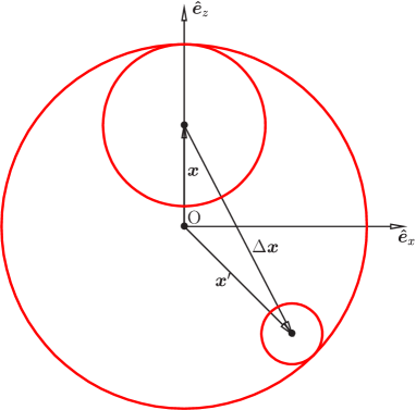
Figure 1: Comoving coordinate system for generalized CMB correlation function, in flat space. All points in the plane shown lie on the past light cone of the observer at O. The outermost circle indicates our last scattering surface. The circles centered on the observers at positions $\bm{x}$ and $\bm{x}^{\prime}$ (and conformal times $\tau=\tau_{0}-|\bm{x}|$ and $\tau^{\prime}=\tau_{0}-|\bm{x}|$ respectively) indicate their last scattering surfaces, which are smaller since recombination occurred in the less distant past according to them. Note that any orientation of the points $\bm{x}$ and $\bm{x}^{\prime}$ in space can be rotated into this plane.

Now we briefly discuss the statistical properties of the coefficients $a_{lm}$ and review the usual definition of cosmic variance. The $a_{lm}$ coefficients at any given point are all independent, but there are spatial and temporal correlations between any pair of coefficients at different points. Assuming Gaussianity of the primordial perturbations, it follows that all of the various $N$-point joint probability distribution functions for the $a_{lm}$ at separate points are (complex) multivariate Gaussians, with covariance matrix $\bm{R}$ given by (note that each index labels both the set of values $l_{i},m_{i}$ and also the point $\mbox{\boldmath$x$}_{i}$ in three dimensional space):

$$R_{ij}=\langle a_{l_{i}m_{i}}(\mbox{\boldmath$x$}_{i})a^{*}_{l_{j}m_{j}}(\mbox{\boldmath$x$}_{j})\rangle=C_{l_{i}m_{i}l_{j}m_{j}}(\mbox{\boldmath$x$}_{i},\mbox{\boldmath$x$}_{j})\ .$$ (5)

Thus given a cosmological model we have the p.d.f of the ensemble from which the $a_{lm}(\mbox{\boldmath$x$})$ are drawn, and the associated ensemble average angular power spectrum harmonics $C_{l}(\tau)$. Then given a set of observations $a^{o}_{lm}(\mbox{\boldmath$x$})$, these ensemble average predictions are typically compared to the observed quantities $C^{o}_{l}(\mbox{\boldmath$x$})=\sum_{m=-l}^{l}|a^{o}_{lm}(\mbox{\boldmath$x$})|^{2}/(2l+1)$ (clearly $\langle C_{l}^{o}(\mbox{\boldmath$x$})\rangle=C_{l}(\tau)$).

On the sky of an observer at time $\tau$, the mean square difference between the observed CMB angular power spectrum $C_{l}^{o}(\bm{x})$ and the ensemble average theoretical power spectrum $C_{l}(\tau)$ is characterized by the cosmic variance

$$\langle[C_{l}^{o}(\mbox{\boldmath$x$})-C_{l}(\tau)]^{2}\rangle=\langle C_{l}^{o}(\mbox{\boldmath$x$})^{2}\rangle-C_{l}(\tau)^{2}\ .$$ (6)

Expanding we obtain

$$\langle C_{l}^{o}(\mbox{\boldmath$x$})^{2}\rangle = \sum_{mm^{\prime}}(2l+1)^{-2}\langle|a^{o}_{lm}(\mbox{\boldmath$x$})|^{2}|a^{o}_{lm^{\prime}}(\mbox{\boldmath$x$})|^{2}\rangle\ .$$ (7)

To evaluate the right hand side, we need the ensemble average of the product of four $a_{lm}$’s. This follows from Gaussianity:

$$\!\!\!\!\!\!\!\!\!\!\!\!\!\!\!\!\langle a_{lm_{1}}(\mbox{\boldmath$x$},\tau)a^{*}_{lm_{2}}(\mbox{\boldmath$x$},\tau)a_{l^{\prime}m_{3}}(\mbox{\boldmath$x$}^{\prime},\tau^{\prime})a^{*}_{l^{\prime}m_{4}}(\mbox{\boldmath$x$}^{\prime},\tau^{\prime})\rangle=\delta_{m_{1}m_{2}}\delta_{m_{3}m_{4}}C_{l}(\tau)\;C_{l^{\prime}}(\tau^{\prime})$$

$$+\;C_{lm_{1}l^{\prime}m_{4}}(\mbox{\boldmath$x$},\mbox{\boldmath$x$}^{\prime})C^{*}_{lm_{2}l^{\prime}m_{3}}(\mbox{\boldmath$x$},\mbox{\boldmath$x$}^{\prime})+C_{lm_{1}l^{\prime},-m_{3}}(\mbox{\boldmath$x$},\mbox{\boldmath$x$}^{\prime})C^{*}_{lm_{2}l^{\prime},-m_{4}}(\mbox{\boldmath$x$},\mbox{\boldmath$x$}^{\prime})\ .$$ (8)

Now setting $l^{\prime}=l$, $\mbox{\boldmath$x$}=\mbox{\boldmath$x$}^{\prime}$, and using $C_{lml^{\prime}m^{\prime}}(\mbox{\boldmath$x$},\mbox{\boldmath$x$})=\delta_{ll^{\prime}}\delta_{mm^{\prime}}C_{l}(\tau)$, we obtain the familiar expression for the cosmic variance associated with each harmonic,

$$\langle C_{l}^{o}(\mbox{\boldmath$x$})^{2}\rangle-C_{l}(\tau)^{2} = \frac{2}{2l+1}\;C_{l}(\tau)^{2}\ .$$ (9)

This quantity captures how much we can expect the measured power spectra to differ from the ensemble average. Note that this expression also follows from the fact that $C_{l}^{o}$ is the sum of squares of independent identical Gaussian random variables, and is therefore distributed as a scaled $\chi^{2}_{2l+1}$ random variable.

Related results concerning the spatial correlations of various quantities can be derived similarly. The ensemble average difference between the $a_{lm}$ measured by separated observers on our past light cone, for example, is characterized by

$$\langle\left|a_{l^{\prime}m^{\prime}}(\mbox{\boldmath$x^{\prime}$})-a_{lm}(\mbox{\boldmath$x$})\right|^{2}\rangle = C_{l^{\prime}}(\tau^{\prime})+C_{l}(\tau)-2\mbox{Re}\;C_{lml^{\prime}m^{\prime}}(\bm{x},\bm{x}^{\prime})\ ,$$ (10)

and the ensemble average difference between the angular power spectrum harmonics as a function of spatial separation is characterized by

$$\left<[C^{o}_{l}(\mbox{\boldmath$x$})-C^{o}_{l^{\prime}}(\mbox{\boldmath$x$}^{\prime})]^{2}\right> = \left<C_{l}^{o}(\mbox{\boldmath$x$})^{2}\right>+\left<C_{l^{\prime}}^{o}(\mbox{\boldmath$x$}^{\prime})^{2}\right>-2\left<C^{o}_{l}(\mbox{\boldmath$x$})C^{o}_{l^{\prime}}(\mbox{\boldmath$x$}^{\prime})\right>$$ (11)

$$= \left[C_{l}(\tau)-C_{l^{\prime}}(\tau^{\prime})\right]^{2}+\frac{2}{2l+1}C_{l}(\tau)^{2}+\frac{2}{2l^{\prime}+1}C_{l^{\prime}}(\tau^{\prime})^{2}$$

$$- \frac{2}{(2l+1)(2l^{\prime}+1)}\sum_{mm^{\prime}}\left[|C_{lml^{\prime}m^{\prime}}(\mbox{\boldmath$x$},\mbox{\boldmath$x$}^{\prime})|^{2}+|C_{lml^{\prime},-m^{\prime}}(\mbox{\boldmath$x$},\mbox{\boldmath$x$}^{\prime})|^{2}\right]\ .$$

We now derive the relationship between the generalized correlation functions and the CMB transfer function. In a flat FRW space, the temperature anisotropy may be Fourier expanded in comoving wavenumber $\bm{k}$ on the three-dimensional hyper-surface of constant $\tau$, $\Sigma_{\tau}$,

$$\Delta(\mbox{\boldmath$x$},\mbox{\boldmath$\hat{n}$},\tau)=\int d^{3}k\;e^{i\mbox{\boldmath$k\cdot x$}}\Delta(\mbox{\boldmath$k$},\mbox{\boldmath$\hat{n}$};\Sigma_{\tau})\ ,$$ (12)

where $\Delta(\mbox{\boldmath$k$},\mbox{\boldmath$\hat{n}$};\Sigma_{\tau})$ is the Fourier transform associated with this hyper-surface only (1995ApJ…455….7M, ).

Since each Fourier mode corresponds in the case of scalar perturbations to a plane wave perturbation which has azimuthal symmetry about $k$, $\Delta(\mbox{\boldmath$k$},\mbox{\boldmath$\hat{n}$};\Sigma_{\tau})$ depends only on $\hat{k}\cdot\hat{n}$ and $|\mbox{\boldmath$k$}|$ and may therefore be expanded in Legendre polynomials:

$$\Delta(\mbox{\boldmath$k$},\mbox{\boldmath$\hat{n}$};\Sigma_{\tau})=\sum_{l=0}^{\infty}(-i)^{l}(2l+1)\Delta_{l}(\mbox{\boldmath$k$},\tau)P_{l}(\mbox{\boldmath$\hat{k}\cdot\hat{n}$})\ .$$ (13)

The $(-i)^{l}$ is included by convention to be consistent with most other authors.  It is convenient to use the addition theorem at this point to express the Legendre polynomials in spherical harmonics, giving

$$\Delta(\mbox{\boldmath$x$},\mbox{\boldmath$\hat{n}$},\tau)=4\pi\int d^{3}k\;e^{i\mbox{\boldmath$k\cdot x$}}\sum_{l=0}^{\infty}(-i)^{l}\;\Delta_{l}(\mbox{\boldmath$k$},\tau)\sum_{m=-l}^{l}Y_{lm}^{*}(\mbox{\boldmath$\hat{k}$})Y_{lm}(\mbox{\boldmath$\hat{n}$})\ .$$ (14)

Employing the orthogonality relation for spherical harmonics $\int d\Omega\;Y_{lm}^{*}(\mbox{\boldmath$\hat{n}$})Y_{l^{\prime}m^{\prime}}(\mbox{\boldmath$\hat{n}$})=\delta_{l^{\prime}l}\delta_{m^{\prime}m}$ (where $d\Omega$ is the integral over solid angle elements centered about direction $\hat{n}$) yields

$$a_{lm}(\mbox{\boldmath$x$},\tau) = \int d\Omega\;\Delta(\mbox{\boldmath$x$},\mbox{\boldmath$\hat{n}$},\tau)Y_{lm}^{*}(\mbox{\boldmath$\hat{n}$})$$

$$= (-i)^{l}\;4\pi\int d^{3}k\;e^{i\mbox{\boldmath$k\cdot x$}}\Delta_{l}(\mbox{\boldmath$k$},\tau)Y_{lm}^{*}(\mbox{\boldmath$\hat{k}$})\ .$$

The correlation function may now be written as

$$C_{lml^{\prime}m^{\prime}}(\mbox{\boldmath$x$},\mbox{\boldmath$x$}^{\prime}) = (-i)^{l-l^{\prime}}\;(4\pi)^{2}\int d^{3}k\;d^{3}k^{\prime}e^{i\mbox{\boldmath$k\cdot x$}}e^{-i\mbox{\boldmath$k^{\prime}\cdot x^{\prime}$}}$$ (16)

$$\quad\quad\quad\quad\quad\quad\langle\Delta_{l}(\mbox{\boldmath$k$},\tau)\Delta_{l^{\prime}}^{*}(\mbox{\boldmath$k$}^{\prime},\tau^{\prime})\rangle Y_{lm}^{*}(\mbox{\boldmath$\hat{k}$})Y_{l^{\prime}m^{\prime}}(\mbox{\boldmath$\hat{k}$}^{\prime})\ .$$

Now since the Boltzmann equation which governs the evolution of the CMB anisotropy $\Delta_{l}(\mbox{\boldmath$k$},\tau)$ is independent of $\hat{k}$ (in linear theory), the $\hat{k}$ dependence comes entirely from the initial conditions, and we may write $\Delta_{l}(\mbox{\boldmath$k$},\tau)$ in terms of the CMB transfer function $\Delta_{l}(k,\tau)$ which is defined by (1995ApJ…455….7M, ):

$$\Delta_{l}(\mbox{\boldmath$k$},\tau)=\phi_{i}(\mbox{\boldmath$k$})\Delta_{l}(k,\tau)\ ,$$ (17)

where $\phi_{i}(\mbox{\boldmath$k$})$ is the initial potential perturbation and $\Delta_{l}(k,\tau)$ is real By the assumption of translational invariance $\phi_{i}(\mbox{\boldmath$k$})$ has a two-point correlation function of the form

$$\langle\phi_{i}(\mbox{\boldmath$k$})\phi^{*}_{i}(\mbox{\boldmath$k$}^{\prime})\rangle=P_{\phi}(k)\;\delta^{3}(\mbox{\boldmath$k$}-\mbox{\boldmath$k$}^{\prime})\ ,$$ (18)

where $P_{\phi}(k)$ is the power spectrum of the primordial (post-inflationary) gravitational potential fluctuations. Then we may write

$$\langle\Delta_{l}(\mbox{\boldmath$k$},\tau)\Delta_{l^{\prime}}^{*}(\mbox{\boldmath$k$}^{\prime},\tau^{\prime})\rangle = \Delta_{l}(k,\tau)\Delta_{l^{\prime}}(k^{\prime},\tau^{\prime})\;P_{\phi}(k)\;\delta^{3}(\mbox{\boldmath$k$}-\mbox{\boldmath$k$}^{\prime})\ .$$ (19)

If we evaluate $C_{lml^{\prime}m^{\prime}}(\mbox{\boldmath$x$},\mbox{\boldmath$x$}^{\prime})$ for $\mbox{\boldmath$x$}=\mbox{\boldmath$x$}^{\prime}$ (and $\tau=\tau^{\prime}$), the covariance matrix is diagonal and the familiar orthogonality relation follows

$$C_{lml^{\prime}m^{\prime}}(\mbox{\boldmath$x$},\mbox{\boldmath$x$})=(4\pi)^{2}\delta_{l^{\prime}l}\delta_{m^{\prime}m}\int k^{2}dk\;\Delta^{2}_{l}(k,\tau)P_{\phi}(k)\equiv\delta_{l^{\prime}l}\delta_{m^{\prime}m}C_{l}(\tau)\ ,$$ (20)

where $C_{l}(\tau)\equiv\langle|a_{lm}(\mbox{\boldmath$x$},\tau)|^{2}\rangle$ is the ensemble average of the $l$ harmonic of the CMB power spectrum according to an observer at conformal time $\tau$. Thus at any given point all of the $a_{lm}$ are independent random variables. Using the addition theorem, we obtain the usual real-space angular correlation function, at any epoch

$$\langle\Delta(\mbox{\boldmath$x$},\mbox{\boldmath$\hat{n}$},\tau)\Delta(\mbox{\boldmath$x$},\mbox{\boldmath$\hat{n}$}^{\prime},\tau)\rangle = \frac{1}{4\pi}\sum_{l}(2l+1)C_{l}(\tau)P_{l}(\mbox{\boldmath$\hat{n}$}\cdot\mbox{\boldmath$\hat{n}$}^{\prime})\ .$$ (21)

With $\mbox{\boldmath$x$}\neq\mbox{\boldmath$x$}^{\prime}$, $\tau\neq\tau^{\prime}$ we obtain a more general expression for the correlation function:

$$C_{lml^{\prime}m^{\prime}}(\mbox{\boldmath$x$},\mbox{\boldmath$x$}^{\prime}) = (-i)^{l-l^{\prime}}\;(4\pi)^{2}\int d^{3}k\;e^{i\mbox{\boldmath$k$}\cdot(\mbox{\boldmath$x$}-\mbox{\boldmath$x$}^{\prime})}$$ (22)

$$\quad\Delta_{l}(k,\tau)\Delta_{l^{\prime}}(k,\tau^{\prime})\;P_{\phi}(k)\;Y_{lm}^{*}(\mbox{\boldmath$\hat{k}$})\;Y_{l^{\prime}m^{\prime}}(\mbox{\boldmath$\hat{k}$})\ .$$

The symmetries stated in equation (II) may be verified from this expression.

We may perform the angular part of the $d^{3}k$ integral in Eqn. (22) by expanding the plane wave piece in spherical Bessel functions (valid in flat space). In a flat FRW space, we are free to manipulate the comoving 3-vectors of events as if we were dealing with position vectors in Euclidean space (see e.g. 1999coph.book…..P , p.71, Eqn. (3.19)). Thus we may define direction vectors $\Delta\mbox{\boldmath$x$}\equiv\mbox{\boldmath$x$}-\mbox{\boldmath$x$}^{\prime}$, $\Delta\mbox{\boldmath$\hat{x}$}\equiv(\mbox{\boldmath$x$}-\mbox{\boldmath$x$}^{\prime})/|\mbox{\boldmath$x$}-\mbox{\boldmath$x$}^{\prime}|$, and expand

$$\exp{\left(i\mbox{\boldmath$k$}\cdot\Delta\mbox{\boldmath$x$}\right)} = \sum_{l^{\prime\prime}=0}^{\infty}(2l^{\prime\prime}+1)i^{l^{\prime\prime}}P_{l^{\prime\prime}}(\mbox{\boldmath$\hat{k}$}\cdot\Delta\mbox{\boldmath$\hat{x}$})j_{l^{\prime\prime}}(k|\Delta\mbox{\boldmath$x$}|)$$ (23)

$$= 4\pi\sum_{l^{\prime\prime}=0}^{\infty}i^{l^{\prime\prime}}j_{l^{\prime\prime}}(k|\Delta\mbox{\boldmath$x$}|)\sum_{m^{\prime\prime}=-l^{\prime\prime}}^{l^{\prime\prime}}Y^{*}_{l^{\prime\prime}m^{\prime\prime}}(\mbox{\boldmath$\hat{k}$})Y_{l^{\prime\prime}m^{\prime\prime}}(\Delta\mbox{\boldmath$\hat{x}$})\ ,$$

where we used the addition theorem to separate the $\hat{k}$ and $\Delta\mbox{\boldmath$\hat{x}$}$ dependence. Then the correlation function becomes

$$C_{lml^{\prime}m^{\prime}}(\mbox{\boldmath$x$},\mbox{\boldmath$x$}^{\prime}) = (4\pi)^{3}\int k^{2}dk\;\Delta_{l}(k,\tau)\Delta_{l^{\prime}}(k,\tau^{\prime})\;P_{\phi}(k)\;(-i)^{l-l^{\prime}}\;(-1)^{m}\;$$ (24)

$$\!\!\!\!\!\!\!\!\!\!\!\!\!\!\!\!\!\!\!\!\!\!\!\!\!\!\!\!\!\!\!\!\!\!\!\!\!\!\times\sum_{l^{\prime\prime}m^{\prime\prime}}i^{l^{\prime\prime}}\;j_{l^{\prime\prime}}(k|\Delta\mbox{\boldmath$x$}|)\;Y_{l^{\prime\prime}m^{\prime\prime}}(\Delta\mbox{\boldmath$\hat{x}$})\int d\Omega_{k}\;Y_{l,-m}(\mbox{\boldmath$\hat{k}$})\;Y_{l^{\prime}m^{\prime}}(\mbox{\boldmath$\hat{k}$})Y^{*}_{l^{\prime\prime}m^{\prime\prime}}(\mbox{\boldmath$\hat{k}$})\ .$$

The angular integral of the product of three spherical harmonics is expressible in terms of the Wigner $3j$ symbols (see e.g. Rose ),

$$\int d\Omega_{k}\;Y_{lm}(\mbox{\boldmath$\hat{k}$})\;Y_{l^{\prime}m^{\prime}}(\mbox{\boldmath$\hat{k}$})Y^{*}_{l^{\prime\prime}m^{\prime\prime}}(\mbox{\boldmath$\hat{k}$})=\sqrt{\frac{(2l+1)(2l^{\prime}+1)(2l^{\prime\prime}+1)}{4\pi}}\;\biggl{(}\begin{array}[]{ccc}l&l^{\prime}&l^{\prime\prime}\\ 0&0&0\end{array}\biggr{)}\biggl{(}\begin{array}[]{ccc}l&l^{\prime}&l^{\prime\prime}\\ m&m^{\prime}&m^{\prime\prime}\end{array}\biggr{)}\ .$$ (29)

The $3j$ symbols are non-zero only if $m+m^{\prime}=m^{\prime\prime}$, and $l,l^{\prime},l^{\prime\prime}$ satisfy the triangle condition that $l^{\prime\prime}$ be equal to one of $l+l^{\prime},l+l^{\prime}-1,\cdots,|l-l^{\prime}|$. The sum over $l^{\prime\prime}$ therefore reduces to a finite sum. We have finally

$$\!\!\!\!\!\!\!\!\!\!\!\!\!\!\!\!\!\!C_{lml^{\prime}m^{\prime}}(\mbox{\boldmath$x$},\mbox{\boldmath$x$}^{\prime})=\;(-i)^{l-l^{\prime}}\;(-1)^{m}\;(4\pi)^{3}\sqrt{\frac{(2l+1)(2l^{\prime}+1)(2l^{\prime\prime}+1)}{4\pi}}$$

$$\times\sum_{l^{\prime\prime}=|l-l^{\prime}|}^{l+l^{\prime}}\biggl{(}\begin{array}[]{ccc}l&l^{\prime}&l^{\prime\prime}\\ 0&0&0\end{array}\biggr{)}\biggl{(}\begin{array}[]{ccc}l&l^{\prime}&l^{\prime\prime}\\ -m&m^{\prime}&m^{\prime}-m\end{array}\biggr{)}\frac{i^{l^{\prime\prime}}}{\sqrt{2l^{\prime\prime}+1}}\;\;K_{l,l^{\prime},l^{\prime\prime}}(|\Delta\mbox{\boldmath$x$}|,\tau,\tau^{\prime})\;Y^{*}_{l^{\prime\prime},m^{\prime}-m}(\Delta\mbox{\boldmath$\hat{x}$})\ ,$$ (34)

where all of the physical information is contained in the kernel

$$K_{l,l^{\prime},l^{\prime\prime}}(|\Delta\mbox{\boldmath$x$}|,\tau,\tau^{\prime})\equiv\int k^{2}dk\;\Delta_{l}(k,\tau)\Delta_{l^{\prime}}(k,\tau^{\prime})\;P_{\phi}(k)\;j_{l^{\prime\prime}}(k|\Delta\mbox{\boldmath$x$}|)\ .$$ (35)

III Transfer functions

To compute $C_{lml^{\prime}m^{\prime}}$ for a given cosmological model we need the CMB transfer function $\Delta_{l}(k,\tau)$. On the large angular scales accessible via the polarization technique, the only significant effects responsible for the temperature anisotropy which need to be included in the transfer function are the Sachs-Wolfe (SW) and integrated Sachs-Wolfe (ISW) effects (1967ApJ…147…73S, ). The SW effect is the anisotropy due to the gravitational potential fluctuations on the last scattering surface, and the associated time dilation effect. The ISW effect arises because, at late times, as the universe is making the transition from the matter dominated phase into the vacuum dominated phase, the fluctuations in the gravitational potential - on scales still in the linear regime - are still evolving with redshift. As photons fall into and climb out of this time changing potential they are red-shifted and thus a temperature anisotropy is generated.

We first consider the transfer function of the SW effect. This is computed by ignoring the physics on scales comparable to the acoustic horizon at the time of recombination, and retaining only the large scale effects. In this limit, the anisotropy is produced solely by the variation in potential $\phi$ (and the consequent gravitational redshift and time dilation effects on the photons) and photon density $\delta_{\gamma}$ across the last scattering shell, ignoring the small scale acoustic waves which give rise to the acoustic peaks in the angular power spectrum. Using the line-of-sight integration method (1996ApJ…469..437S, ), the SW temperature anisotropy is given in real space by

$$\Delta(\mbox{\boldmath$x$},\mbox{\boldmath$n$},\tau) = \int_{0}^{\tau}d\chi^{\prime}\;\dot{\zeta}(\tau-\chi^{\prime})\;\left[\frac{1}{4}\delta_{\gamma}(\chi^{\prime}\mbox{\boldmath$\hat{n}$})+\phi(\chi^{\prime}\mbox{\boldmath$\hat{n}$})\right]\ .$$ (36)

Here $\chi^{\prime}$ is the comoving distance measured along the past light cone of the observer at $(\mbox{\boldmath$x$},\tau)$, in the direction $n$. The visibility function is defined by $\zeta(\tau)\equiv e^{-\tau_{\rm C}(\tau)}$, with Thomson optical depth $\tau_{\rm C}(\tau)=\int_{0}^{\tau}d\chi^{\prime}a(\tau-\chi^{\prime})n_{e}(\tau-\chi^{\prime})\sigma_{\rm T}$ (here and elsewhere a dot means a derivative with respect to conformal time $\tau$).

In the Sachs-Wolfe approximation (valid on scales much larger than the acoustic horizon), and assuming adiabatic initial conditions, a perturbative analysis of the equations of motion shows that $\delta_{\gamma}=-\frac{8}{3}\phi$, and that in Fourier space the evolution of the potential is given by $\phi(\mbox{\boldmath$k$},\tau)=\frac{9}{10}\phi_{i}(\mbox{\boldmath$k$})$ (see, for example, 2002PhRvD..65l3008B ; 2003Orion.314S..33. ). The factor of $9/10$ accounts for the evolution of the transfer function between radiation and matter domination (in the case of adiabatic initial conditions). Decomposing the plane waves (working here in flat space) into spherical waves, we obtain

$$\Delta_{l}(k,\tau) = \frac{3}{10}\int_{0}^{\tau}d\chi^{\prime}\;\dot{\zeta}(\tau-\chi^{\prime})\;j_{l}(k\chi^{\prime})\ .$$ (37)

The visibility function $\zeta$ contains the physics of recombination. It rises rapidly during recombination from $0$ to $1$, with derivative sharply peaked about the time of recombination, $\tau_{r}$ (1995ApJ…439..503D, ). The effect of the finite thickness of the last scattering shell can only influence the radiation field on rather small scales, so for times well after recombination, and for low $l$, we may assume that recombination occurred instantaneously at time $\tau_{r}$. In this limit we may take $\zeta$ to be a delta function centered on $\tau_{r}$, and the transfer function reduces to

$$\Delta_{l}(k,\tau)=\frac{3}{10}j_{l}[k(\tau-\tau_{r})]\ .$$ (38)

Taking the usual power law form $P_{\phi}(k)=Ak^{n-4}$ ($n=1$ gives the scale-invariant Harrison-Zeldovich spectrum) with an arbitrary amplitude $A$ (with dimensions of
$\left(c/H_{0}\right)^{n-1}$), with the transfer function in equation (38) the integral in equation (20) may be done analytically, yielding the well known Sachs-Wolfe expression for the angular power spectrum at low $l$ and $n<3$ (see for example 1999coph.book…..P ):

$$C_{l}(\tau) = A(4\pi)^{2}\left(\frac{3}{10}\right)^{2}\int_{0}^{\infty}k^{2}dk\;k^{n-4}j_{l}^{2}\left[k(\tau-\tau_{r})\right]$$ (39)

$$= A(4\pi)^{2}\left(\frac{3}{10}\right)^{2}\pi 2^{n-4}\frac{\Gamma(3-n)\Gamma(\frac{2l+n-1}{2})}{\Gamma^{2}(\frac{4-n}{2})\Gamma(\frac{2l+5-n}{2})}\;(\tau-\tau_{r})^{1-n}\ .$$

Note that if $n=1$, this expression has no time dependence. This is a manifestation of the scale invariance property of the $n=1$ case.

In the general case including the ISW effect (and assuming a flat universe), the CMB transfer function is given by a generalization of Eqn. (36), the line of sight integral:

$$\Delta(\mbox{\boldmath$x$},\mbox{\boldmath$n$},\tau) = \int_{0}^{\tau}d\chi^{\prime}\;\dot{\zeta}(\tau-\chi^{\prime})\;\left[\frac{1}{4}\delta_{\gamma}(\chi^{\prime}\mbox{\boldmath$\hat{n}$})+\phi(\chi^{\prime}\mbox{\boldmath$\hat{n}$})\right]$$ (40)

$$\quad\quad\quad\quad+\int_{0}^{\tau}d\chi^{\prime}\;\zeta(\tau-\chi^{\prime})\;2\dot{\phi}(\chi^{\prime}\mbox{\boldmath$\hat{n}$})\ .$$

In linear theory, the growth of the amplitude of the potential perturbations is governed by the growth function $D_{+}(\tau)$ of the dark matter perturbation The evolution of the potential perturbation in the adiabatic case is then given by $\phi(\mbox{\boldmath$k$},\tau)=\frac{9}{10}\phi_{i}(\mbox{\boldmath$k$})D_{+}(\tau)/a(\tau)$.

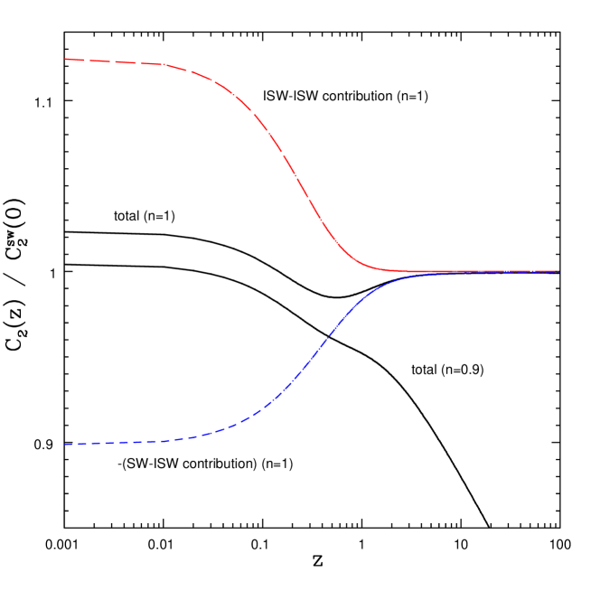
Figure 2: A plot of $C_{2}(z)$, including both the SW and ISW effects, normalized to the value of the SW contribution at $z=0$. The growth function was computed in a $\Lambda$CDM model with $(\Omega_{\Lambda},\Omega_{m})=(0.7,0.3)$. The upper solid black curve is for the case of power spectral index $n=1$, and the lower solid black curve for $n=0.9$. The dashed upper and lower curves curves show the contributions to the $n=1$ case from the ISW-ISW term and the SW-ISW interference term respectively. These two tend to cancel. (Note that the interference term is negative, and its magnitude is plotted here).

In the case of a flat universe with only non-relativistic matter and vacuum energy, the solution for the growth function, normalized to $D_{+}=a$ at early times, has the simple form (1977MNRAS.179..351H, ):

$$D_{+}(\tau)=\frac{5}{2}\Omega_{m}\frac{\sqrt{\Omega_{m}+\Omega_{\Lambda}a(\tau)^{3}}}{a(\tau)^{3/2}}\int_{0}^{a(\tau)}X^{3/2}(a^{\prime})\;da^{\prime}$$

$$\mbox{where}\;\;\;\;\;\;\;\;\;X(a)=\frac{a}{\Omega_{m}+\Omega_{\Lambda}a^{3}}\ .$$ (41)

In the instantaneous recombination approximation, this leads to the following CMB transfer function

$$\Delta_{l}(k,\tau)=\frac{3}{10}j_{l}\left[k(\tau-\tau_{r})\right]+\frac{9}{5}\int_{0}^{\tau-\tau_{r}}d\chi^{\prime}\;j_{l}(k\chi^{\prime})\;\left.\frac{\partial}{\partial\tau}\frac{D_{+}}{a}\right|_{\tau-\chi^{\prime}}\ ,$$ (42)

where the time derivative in the integrand is evaluated at time $\tau-\chi^{\prime}$.

In the kernel $K_{ll^{\prime}l^{\prime\prime}}$, the product of two transfer functions appears. Thus there are three terms, a contribution entirely from the SW effect, an “interference” contribution from both the SW and ISW effects, and a contribution entirely from the ISW effect. Since the ISW part of the transfer function is usually negative, the interference term tends to cancel the third term. This is illustrated in Fig. 2, which shows the redshift dependence of the CMB harmonic $C_{2}$ in a $\Lambda$CDM model with $(\Omega_{\Lambda},\Omega_{m})=(0.7,0.3)$, and various values of the power spectral index $n$.

IV Scattering of CMB quadrupole

In this section we consider the generation of polarization by scattering of the intrinsic CMB quadrupole from electrons in a galaxy cluster, which we idealize as a concentrated clump of stationary electrons with a Thomson optical depth $\tau_{\rm C}$, at a specific angular point on the sky.

The Stokes parameters of the radiation scattered into the line of sight to the cluster are functions of the quadrupole anisotropy in the local CMB radiation field at the cluster. This is characterized by the coefficients $a_{2m}(\bm{x})$ of the spherical harmonic expansion of the fractional temperature anisotropy of the radiation field, which are functions of the spatial position of the cluster in comoving coordinates denoted $\bm{x}$ (see §II for a description of this coordinate system). The direction vector of the line of sight from the observer at $z=0$ to the cluster is $\hat{x}$. The coordinate system used is illustrated in Fig. 3.

In terms of the general set of coefficients $a_{lm}(\bm{x})$, we may write the brightness temperature of the incident CMB radiation field at the cluster as a function of the direction vector $\hat{n}$ of the incoming photon as viewed from the cluster:

$$I(\mbox{\boldmath$\hat{n}$},\bm{x})=T_{\rm CMB}(\tau)\sum_{lm}a_{lm}(\mbox{\boldmath$x$})Y_{lm}(\mbox{\boldmath$\hat{n}$})\ ,$$ (43)

where $\tau=\tau_{0}-|\mbox{\boldmath$x$}|$ is the conformal time of the scattering events. Since the primary anisotropy has a blackbody spectrum, there is no frequency dependence in $I(\mbox{\boldmath$\hat{n}$},\bm{x})$.

We assume that the incident CMB radiation is unpolarized, which is sufficient to compute the lowest order polarization signal generated by the quadrupole anisotropy (there are relativistic corrections to the effect described here in the case of a cluster with a peculiar velocity with respect to the CMB, as discussed by 2002PhRvD..65j3001C , which turn out to be negligible).

The brightness temperature polarization matrix $I_{ij}\sim\langle E_{i}E_{j}\rangle$ of the radiation scattered into the line of sight is given in the Thomson limit by the following equation:

$$I_{ij}(\bm{x}) = \frac{3\tau_{\rm C}}{16\pi}\;\left(\delta_{ik}-\hat{x}_{i}\hat{x}_{k}\right)\left(\delta_{jl}-\hat{x}_{j}\hat{x}_{l}\right)\int d\Omega^{\prime}\;I(\mbox{\boldmath$\hat{n}$},\bm{x})\left(\delta_{kl}-\hat{n}_{k}\hat{n}_{l}\right)\ ,$$ (44)

where $d\Omega^{\prime}$ is the solid angle element about the $\hat{n}$ direction. A self-contained derivation of this form of the transfer equation is provided in Appendix A. The primed solid angle element $d\Omega^{\prime}$ is associated with the unprimed direction vector $\hat{\bm{n}}$ since we wish to reserve $d\Omega$ for the polar angles of the cluster on the sky.

We now define a polarization basis to define the Stokes parameters of the radiation incident at the observer from a cluster in any direction on the sky. We denote the polarization basis vectors as $\mbox{\boldmath$\hat{e}$}_{1},\mbox{\boldmath$\hat{e}$}_{2}$ and leave these unspecified for the moment. The Stokes parameters measured in the $\mbox{\boldmath$\hat{e}$}_{1},\mbox{\boldmath$\hat{e}$}_{2}$ basis at our position due to scattering in the cluster at comoving position $\bm{x}$ are then:

$$I(\mbox{\boldmath$x$})+Q(\mbox{\boldmath$x$}) = 2I_{ij}(\bm{x})\;\hat{e}_{1,i}\hat{e}_{1,j}\ ,$$

$$I(\mbox{\boldmath$x$})-Q(\mbox{\boldmath$x$}) = 2I_{ij}(\bm{x})\;\hat{e}_{2,i}\hat{e}_{2,j}\ ,$$

$$U(\mbox{\boldmath$x$}) = 2I_{ij}(\bm{x})\;\hat{e}_{1,i}\hat{e}_{2,j}\ .$$ (45)

Note that we may ignore the Stokes $V$ parameter - it remains zero since no circular polarization is generated by Thomson scattering.

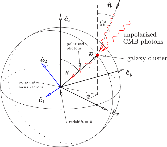
Figure 3: Illustrates the coordinate system used to describe the generation of polarization by Thomson scattering. The CMB incident on a cluster at comoving position $x$, which we approximate as unpolarized, is Thomson scattered and re-radiated by free electrons in the cluster, producing partially polarized radiation scattered into the line of sight. At the observer position (redshift $z=0$) the radiation is decomposed into Stokes parameters with the polarization basis vectors $\hat{\bm{e}}_{1},\hat{\bm{e}}_{2}$ indicated (defined in equation (55). The CMB radiation incident on the cluster at $\bm{x}$ is decomposed into spherical harmonics defined with respect to polar coordinates $\theta^{\prime}$ and $\phi^{\prime}$. Only the $l=2$ harmonics of the incident radiation field generate polarization.

On substitution of Eqn. (43) we find

$$Q(\mbox{\boldmath$x$}) = \frac{3\tau_{\rm C}}{16\pi}T_{\rm CMB}(\tau)\sum_{lm}a_{lm}(\mbox{\boldmath$x$})\int d\Omega^{\prime}\;Y_{lm}(\mbox{\boldmath$\hat{n}$})\;\left[(\mbox{\boldmath$\hat{e}$}_{2}\cdot\mbox{\boldmath$\hat{n}$})^{2}-(\mbox{\boldmath$\hat{e}$}_{1}\cdot\mbox{\boldmath$\hat{n}$})^{2}\right]\ ,$$

$$U(\mbox{\boldmath$x$}) = -\frac{3\tau_{\rm C}}{8\pi}T_{\rm CMB}(\tau)\sum_{lm}a_{lm}(\mbox{\boldmath$x$})\int d\Omega^{\prime}\;Y_{lm}(\mbox{\boldmath$\hat{n}$})(\mbox{\boldmath$\hat{e}$}_{1}\cdot\mbox{\boldmath$\hat{n}$})(\mbox{\boldmath$\hat{e}$}_{2}\cdot\mbox{\boldmath$\hat{n}$})\ .$$ (46)

To perform the angular integral we need to expand the integrands in equations (IV) in spherical harmonics by expressing $\hat{n}$ in polar coordinates. In polar coordinates about the $\hat{z}$ axis, the Cartesian components of the direction vectors are taken to be:

$$\hat{n} = (\hat{n}_{x},\hat{n}_{y},\hat{n}_{z})=(\sin\theta^{\prime}\cos\phi^{\prime},\sin\theta^{\prime}\sin\phi^{\prime},\cos\theta^{\prime})\ ,$$

$$\hat{x} = (\hat{x}_{x},\hat{x}_{y},\hat{x}_{z})=(\sin\theta\cos\phi,\sin\theta\sin\phi,\cos\theta)\ .$$ (47)

We use the following method. Any spherical harmonic can be expanded in terms of the complex quantities $(z_{1},z_{2},z_{3})=(\sin\theta^{\prime}e^{i\phi^{\prime}},\sin\theta^{\prime}e^{-i\phi^{\prime}},\cos\theta^{\prime})$ (see for example the discussion of spherical harmonics in ByronFuller ). In terms of these functions we may write $\mbox{\boldmath$\hat{n}$}=((z_{1}+z_{2})/2,i(z_{2}-z_{1})/2,z_{3})$. Note that $z_{2}=z_{1}^{*},\;z_{3}^{*}=z_{3},\;z_{1}z_{2}=1-z_{3}^{2}$. It is also convenient to define

$$\mbox{\boldmath$\hat{e}$}_{+} \equiv \mbox{\boldmath$\hat{e}$}_{x}+i\mbox{\boldmath$\hat{e}$}_{y}\ ,$$

$$\mbox{\boldmath$\hat{e}$}_{-} \equiv \mbox{\boldmath$\hat{e}$}_{x}-i\mbox{\boldmath$\hat{e}$}_{y}\ .$$ (48)

Then for instance we have

$$\mbox{\boldmath$\hat{e}$}_{1}\cdot\mbox{\boldmath$\hat{n}$}=\frac{z_{1}}{2}\;\mbox{\boldmath$\hat{e}$}_{1}\cdot\mbox{\boldmath$\hat{e}$}_{-}+\frac{z_{2}}{2}\;\mbox{\boldmath$\hat{e}$}_{1}\cdot\mbox{\boldmath$\hat{e}$}_{+}+z_{3}\;\mbox{\boldmath$\hat{e}$}_{1}\cdot\mbox{\boldmath$\hat{e}$}_{z}$$ (49)

The $l=2$ spherical harmonics may be written as functions quadratic in the $z$’s as follows:

$$Y_{2,0} = \sqrt{\frac{5}{4\pi}}\left(\frac{3}{2}z_{3}^{2}-\frac{1}{2}\right),$$

$$vY_{2,1} = -\sqrt{\frac{15}{8\pi}}\;z_{1}z_{3},\;\;\;\;\;\;\;Y_{2,-1}=\sqrt{\frac{15}{8\pi}}\;z_{2}z_{3}$$

$$Y_{2,2} = \frac{1}{4}\sqrt{\frac{15}{2\pi}}\;z_{1}^{2},\;\;\;\;\;\;\;Y_{2,-2}=\frac{1}{4}\sqrt{\frac{15}{2\pi}}\;z_{2}^{2}\ .$$ (50)

Then we can decompose the integrands into spherical harmonics by expanding the integrands in equation (IV) in the $z$’s using expressions like (49) and comparing with the expressions for $Y_{2m}$ above. (Note that in performing this calculation, it is necessary to use the relation $z_{1}z_{2}=1-z_{3}^{2}$ to eliminate one of the coefficients $(z_{1},z_{2},z_{3})$). We find the following manifestly real result for the integrands of $Q$ and $U$:

$$(\mbox{\boldmath$\hat{e}$}_{2}\cdot\mbox{\boldmath$\hat{n}$})^{2}-(\mbox{\boldmath$e$}_{1}\cdot\mbox{\boldmath$\hat{n}$})^{2} = \sqrt{\frac{8\pi}{5}}\sum_{m=-2}^{2}Q_{m}(\mbox{\boldmath$\hat{x}$})Y_{2,m}(\mbox{\boldmath$\hat{n}$})\ ,$$

$$-2(\mbox{\boldmath$\hat{e}$}_{1}\cdot\mbox{\boldmath$\hat{n}$})(\mbox{\boldmath$e$}_{2}\cdot\mbox{\boldmath$\hat{n}$}) = \sqrt{\frac{8\pi}{5}}\sum_{m=-2}^{2}U_{m}(\mbox{\boldmath$\hat{x}$})Y_{2,m}(\mbox{\boldmath$\hat{n}$})\ .$$ (51)

The coefficients $Q_{m},U_{m}$ appearing in this expression are the following functions of the arbitrary polarization basis vectors chosen by the observer, which in turn are functions of the cluster direction on the sky (so $Q_{m},\,U_{m}$ are written as functions of the cluster direction vector $\hat{\bm{x}}$, which will become explicit once a polarization basis is chosen):

$$Q_{0}(\mbox{\boldmath$\hat{x}$}) = -\frac{1}{\sqrt{2}}\left[(\mbox{\boldmath$\hat{e}$}_{1}\cdot\mbox{\boldmath$\hat{e}$}_{z})^{2}-(\mbox{\boldmath$e$}_{2}\cdot\mbox{\boldmath$\hat{e}$}_{z})^{2}\right]\ ,$$

$$Q_{1}(\mbox{\boldmath$\hat{x}$}) = \frac{1}{\sqrt{3}}\left[(\mbox{\boldmath$\hat{e}$}_{-}\cdot\mbox{\boldmath$\hat{e}$}_{1})(\mbox{\boldmath$\hat{e}$}_{z}\cdot\mbox{\boldmath$\hat{e}$}_{1})-(\mbox{\boldmath$\hat{e}$}_{-}\cdot\mbox{\boldmath$\hat{e}$}_{2})(\mbox{\boldmath$e$}_{z}\cdot\mbox{\boldmath$\hat{e}$}_{2})\right]\ ,$$

$$Q_{2}(\mbox{\boldmath$\hat{x}$}) = \frac{1}{2\sqrt{3}}\left[(\mbox{\boldmath$\hat{e}$}_{-}\cdot\mbox{\boldmath$\hat{e}$}_{2})^{2}-(\mbox{\boldmath$\hat{e}$}_{-}\cdot\mbox{\boldmath$\hat{e}$}_{1})^{2}\right]\ ,$$ (52)

and

$$U_{0}(\mbox{\boldmath$\hat{x}$}) = -\sqrt{2}(\mbox{\boldmath$\hat{e}$}_{1}\cdot\mbox{\boldmath$\hat{e}$}_{z})(\mbox{\boldmath$e$}_{2}\cdot\mbox{\boldmath$\hat{e}$}_{z})\ ,$$

$$U_{1}(\mbox{\boldmath$\hat{x}$}) = \frac{1}{\sqrt{3}}\left[(\mbox{\boldmath$\hat{e}$}_{-}\cdot\mbox{\boldmath$e$}_{1})(\mbox{\boldmath$\hat{e}$}_{z}\cdot\mbox{\boldmath$\hat{e}$}_{2})+(\mbox{\boldmath$\hat{e}$}_{-}\cdot\mbox{\boldmath$\hat{e}$}_{2})(\mbox{\boldmath$e$}_{z}\cdot\mbox{\boldmath$\hat{e}$}_{1})\right]\ ,$$

$$U_{2}(\mbox{\boldmath$\hat{x}$}) = -\frac{1}{\sqrt{3}}(\mbox{\boldmath$\hat{e}$}_{-}\cdot\mbox{\boldmath$e$}_{1})(\mbox{\boldmath$\hat{e}$}_{-}\cdot\mbox{\boldmath$\hat{e}$}_{2})\ .$$ (53)

Also, we define the quantities with negative $m$ by the relations

$$Q_{-m}(\mbox{\boldmath$\hat{x}$}) \equiv (-1)^{m}Q_{m}^{*}(\mbox{\boldmath$\hat{x}$})\ ,$$

$$U_{-m}(\mbox{\boldmath$\hat{x}$}) \equiv (-1)^{m}U_{m}^{*}(\mbox{\boldmath$\hat{x}$})\ .$$ (54)

We specialize now to a particular choice of of polarization basis vectors. A suitable choice is

$$\mbox{\boldmath$\hat{e}$}_{1}=\frac{\mbox{\boldmath$\hat{x}$}\times\mbox{\boldmath$\hat{e}$}_{z}}{\sqrt{1-\mu^{2}}}\ ,\quad\mbox{\boldmath$\hat{e}$}_{2}=\frac{\mbox{\boldmath$\hat{e}$}_{z}-\mu\mbox{\boldmath$\hat{x}$}}{\sqrt{1-\mu^{2}}}\ ,$$ (55)

where $\mu=\mbox{\boldmath$\hat{x}$}\cdot\mbox{\boldmath$\hat{e}$}_{z}=\cos\theta$, so that the Stokes parameters $Q,U$ are defined with respect to the plane containing the $\mbox{\boldmath$\hat{e}$}_{z}$ axis and the photon direction $-\mbox{\boldmath$\hat{x}$}$ (see Fig. 3). In this polarization basis the coefficients $Q_{m}$, $U_{m}$ are

$$Q_{0}(\mbox{\boldmath$\hat{x}$}) = \frac{1}{\sqrt{2}}\sin^{2}\theta\ ,$$

$$Q_{1}(\mbox{\boldmath$\hat{x}$}) = \frac{1}{\sqrt{3}}\cos\theta\sin\theta e^{-i\phi}\ ,$$

$$Q_{2}(\mbox{\boldmath$\hat{x}$}) = \frac{1}{2\sqrt{3}}(1+\cos^{2}\theta)e^{-2i\phi}\ ,$$

$$U_{0}(\mbox{\boldmath$\hat{x}$}) = 0\ ,$$

$$U_{1}(\mbox{\boldmath$\hat{x}$}) = \frac{i}{\sqrt{3}}\sin\theta e^{-i\phi}\ ,$$

$$U_{2}(\mbox{\boldmath$\hat{x}$}) = \frac{i}{\sqrt{3}}\cos\theta e^{-2i\phi}\ ,$$ (56)

where $\theta$ is the polar angle between $\bm{x}$ and the $\mbox{\boldmath$\hat{e}$}_{z}$ axis and $\phi$ is the azimuthal angle between the projection of $\bm{x}$ on the $(\mbox{\boldmath$\hat{e}$}_{x},\mbox{\boldmath$\hat{e}$}_{y})$ plane and the $\mbox{\boldmath$\hat{e}$}_{x}$ axis.

The Stokes parameters may now finally be expressed as a linear combination of the $a_{2m}(\bm{x})$, with polar axis $\mbox{\boldmath$\hat{e}$}_{z}$. Angular integration picks out the five coefficients $a_{2m}$ of the primary anisotropy:

$$Q(\mbox{\boldmath$x$}) = \tau_{\rm C}P_{0}\sum_{m=-2}^{2}Q_{m}(\mbox{\boldmath$\hat{x}$})a_{2m}(\mbox{\boldmath$x$})\ ,$$

$$U(\mbox{\boldmath$x$}) = \tau_{\rm C}P_{0}\sum_{m=-2}^{2}U_{m}(\mbox{\boldmath$\hat{x}$})a_{2m}(\mbox{\boldmath$x$})\ ,$$ (57)

where $P_{0}\equiv\frac{3}{4\sqrt{10\pi}}T_{\rm CMB}(\tau)$. Note that this depends on conformal time, but the fractional distortion in the Stokes parameters is redshift independent. Also, it turns out that

$$Q_{m}+iU_{m}=\frac{4}{3}\sqrt{\frac{3\pi}{5}}\;{{}_{2}}Y^{*}_{2m}(\theta,\phi)\ ,$$ (58)

where ${{}_{2}}Y_{lm}$ is the spin-weighted spherical harmonic of spin 2 (see e.g. 1997PhRvD..56..596H ). Thus we may write

$$Q(\bm{x})\pm iU(\bm{x})=-\frac{6}{20}\sqrt{\frac{2}{3}}\tau_{\rm C}T_{\rm CMB}(\tau)\,\sum_{m=-2}^{2}{{}_{\pm 2}}Y_{2m}(\mbox{\boldmath$\hat{x}$})\;a_{2m}(\bm{x})\ .$$ (59)

Finally in this section, we quote the following properties of $Q_{m},U_{m}$, which are needed in §V (these are derived using the explicit forms in Eqn. (IV)):

$$\sum_{m=-2}^{2}|Q_{m}(\mbox{\boldmath$\hat{x}$}_{i})|^{2}=\sum_{m=-2}^{2}|U_{m}(\mbox{\boldmath$\hat{x}$}_{i})|^{2}=\frac{2}{3}\ ,$$

$$\sum_{m=-2}^{2}Q_{m}(\mbox{\boldmath$\hat{x}$}_{i})U^{*}_{m}(\mbox{\boldmath$\hat{x}$}_{i})=0\ ,$$

$$\sum_{m=-2}^{2}(-1)^{m}Q_{m}(\mbox{\boldmath$\hat{x}$}_{i})Q^{*}_{m}(\mbox{\boldmath$\hat{x}$}_{i})=\frac{2}{3}\left[1-\frac{1}{2}\sin^{2}2\theta_{i}\right]\ ,$$

$$\sum_{m=-2}^{2}(-1)^{m}U_{m}(\mbox{\boldmath$\hat{x}$}_{i})U^{*}_{m}(\mbox{\boldmath$\hat{x}$}_{i})=\frac{2}{3}\cos 2\theta_{i}\ ,$$

$$\sum_{m=-2}^{2}(-1)^{m}Q_{m}(\mbox{\boldmath$\hat{x}$}_{i})U^{*}_{m}(\mbox{\boldmath$\hat{x}$}_{i})=0\ .$$ (60)

V Statistics of the cluster polarization signal

Now we consider the information obtainable from measurements of the CMB polarization signal (due to scattering of the CMB quadrupole) from galaxy clusters at various redshifts and lines of sight. Assuming that the redshifts of each cluster can be obtained, this allows mapping, in principle, of a particular linear combination of $a_{lm}$ over a significant portion of our past light cone. Galaxy clusters at similar redshifts and on lines of sight separated by small angles will produce polarization signals with Stokes parameters which are strongly correlated. Widely separated clusters produce uncorrelated signals — and it is the combination of these uncorrelated signals that gets around the cosmic variance bound.

Using Eqn. (IV), the two-point correlation function $\langle Q(\mbox{\boldmath$x$})Q(\mbox{\boldmath$x$}^{\prime})\rangle$, of the Stokes parameters, as defined in the basis Eqn. (55), due to two clusters at general comoving positions $\bm{x},\bm{x}^{\prime}$ with Thomson optical depths $\tau_{\rm C},\tau_{\rm C}^{\prime}$ is given by

$$\!\!\!\!\!\!\!\!\!\!\!\!\langle Q(\mbox{\boldmath$x$})Q(\mbox{\boldmath$x$}^{\prime})\rangle=\tau_{\rm C}\tau_{\rm C}^{\prime}P_{0}^{2}\sum_{m,m^{\prime}=-2}^{2}Q_{m}(\mbox{\boldmath$\hat{x}$})Q^{*}_{m^{\prime}}(\mbox{\boldmath$\hat{x}$}^{\prime})\;C_{2m2m^{\prime}}(\mbox{\boldmath$x$},\mbox{\boldmath$x$}^{\prime})\ ,$$ (61)

and similarly for $\langle U(\mbox{\boldmath$x$})U(\mbox{\boldmath$x$}^{\prime})\rangle$ and $\langle Q(\mbox{\boldmath$x$})U(\mbox{\boldmath$x$}^{\prime})\rangle$.

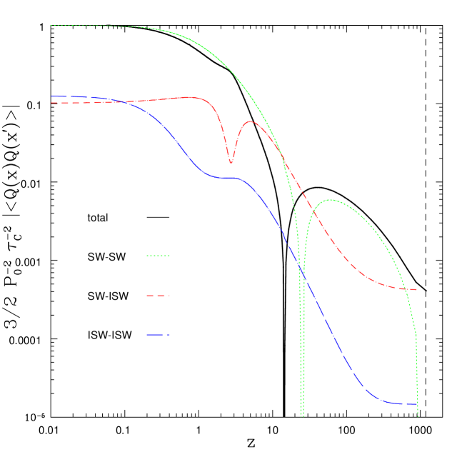
Figure 4: Normalized magnitude of the two-point correlation function of the Stokes Q parameter, $\frac{3}{2}P_{0}^{-2}\tau_{\rm C}^{-2}|\langle Q(\mbox{\boldmath$x$})Q(\mbox{\boldmath$x$}^{\prime})\rangle|/C_{2}(\tau_{0})$, where $\bm{x}$ is taken to be at redshift $z=0$ and $\bm{x}^{\prime}$ is a point at redshift $z$ in the plane orthogonal to $\hat{\bm{z}}$. The growth function was computed with cosmological parameters $\Omega_{m}=0.35$, $\Omega_{\Lambda}=0.65$, $n=1$. (Note that the dip in the interference term, which occurs at $z\approx 3$, is not a zero crossing).

The two-point correlation function $\langle Q(\mbox{\boldmath$x$})Q(\mbox{\boldmath$x$}^{\prime})\rangle$, for points lying on the same line of sight, is shown in Fig. 4, which was computed with cosmological parameters $\Omega_{m}=0.35$, $\Omega_{\Lambda}=0.65$, $n=1$. The solid black curve is the total correlation, and the other curves show the contributions from the SW and ISW terms, and their interference term. Note that the interference term is negative - its magnitude is shown here. Only the SW contribution has a genuine zero crossing. The vertical dashed line indicates the time of (instantaneous) recombination. Note that the SW part of the correlation passes through zero at redshift $\approx 10$, since at redshifts higher than this $\bm{x}^{\prime}$ is in a region of the universe separated from the origin by a comoving distance greater than $c/(2H_{0})$, and thus the $l=2$ correlations die off rapidly.

As $\mbox{\boldmath$x$}\rightarrow\mbox{\boldmath$x$}^{\prime}$, $\langle a_{2m}(\mbox{\boldmath$x$})a^{*}_{2m^{\prime}}(\mbox{\boldmath$x$}^{\prime})\rangle\rightarrow C_{2}(\tau)\delta_{mm^{\prime}}$, therefore

$$\langle Q(\mbox{\boldmath$x$})^{2}\rangle = \langle U(\mbox{\boldmath$x$})^{2}\rangle=\frac{2}{3}\tau_{\rm C}^{2}P^{2}_{0}\;C_{2}(\tau)\ ,$$

$$\langle Q(\mbox{\boldmath$x$})U(\mbox{\boldmath$x$})\rangle = 0\ .$$ (62)

Thus the ensemble average polarization magnitude due to the scattering of the CMB quadrupole is:

$$\langle\Pi(\bm{x})^{2}\rangle\equiv\frac{\langle Q(\mbox{\boldmath$x$})^{2}\rangle+\langle U(\mbox{\boldmath$x$})^{2}\rangle}{T_{\rm CMB}(\tau)^{2}}=\frac{4}{3}\tau_{\rm C}^{2}\left(\frac{P_{0}}{T_{\rm CMB}(\tau)}\right)^{2}\;C_{2}(\tau)\ .$$ (63)

The quadrupole $Q_{2}$ is conventionally defined by $C_{2}=(4\pi/5)Q_{2}^{2}$. Thus the root mean square polarization magnitude is given by (recall $P_{0}\equiv\frac{3}{4\sqrt{10\pi}}T_{\rm CMB}(\tau)$)

$$\langle P\rangle\equiv\sqrt{\langle\Pi(\bm{x})^{2}\rangle}=\frac{\sqrt{6}}{10}\tau_{\rm C}Q_{2}\ ,$$ (64)

as obtained by 2003PhRvD..67f3505C . In a $\Lambda$CDM model, $\langle P\rangle\approx 5\tau_{\rm C}\,\mu$K (at zero redshift), so the magnitude of this signal is comparable to that of the other SZ polarization effects.

Now the relations Eqn. (V) suggest estimators $\widehat{C}^{Q}_{2}(\tau)$ and $\widehat{C}^{U}_{2}(\tau)$ of $C_{2}(\tau)$, given the measured Stokes parameters of $N$ clusters at the same redshift $z(\tau)$ on lines of sight $\hat{\bm{x}}_{i}$ with optical depths $\tau_{C,i}$ $(i=1,\cdots\!,N)$, which beat the cosmic variance limit:

$$\widehat{C}^{Q}_{2}(\tau) \equiv \frac{3}{2}P^{-2}_{0}\sum_{i}W_{i}\;Q(\bm{x}_{i})^{2}\ ,$$

$$\widehat{C}^{U}_{2}(\tau) \equiv \frac{3}{2}P^{-2}_{0}\sum_{i}W_{i}\;U(\bm{x}_{i})^{2}\ .$$ (65)

Note that these are non-optimal, coordinate-dependent estimators. In future work it would be interesting to construct optimal estimators of the power at a given scale, given the cluster polarization data, but we do not attempt that here. For the mean of these estimators to equal $C_{2}(\tau)$, the weights $W_{i}$ must be chosen to satisfy

$$\sum_{i}W_{i}\;\tau^{2}_{C,i}=1\ .$$ (66)

We will consider the simple choice

$$W_{i}=\frac{\tau_{C,i}^{n-2}}{\sum_{j}\tau_{C,j}^{n}}\ .$$ (67)

Note that $n=0$ would be a bad choice since it gives more weight to clusters producing weaker signals, reducing the signal to noise. A better choice is the uniform weighting $n=2$.

The cosmic variance limit on these estimators is determined by the variances (with $X,X^{\prime}$ indicating either $Q$ or $U$)

$$\mbox{Var}\;\widehat{C}_{2}^{X}(\tau) = \frac{9}{4}P_{0}^{-4}\sum_{ij}W_{i}\;W_{j}\;\langle X(\bm{x}_{i})^{2}X(\bm{x}_{j})^{2}\rangle\ .$$ (68)

The sum over $i,j$ may be broken into a contribution from clusters at the same location, $\mbox{Var}_{1}(X)$, and a contribution from clusters at separate locations, $\mbox{Var}_{2}(X,X)$:

$$\mbox{Var}\;\widehat{C}^{X}_{2}(\tau)=\mbox{Var}_{1}(X)+\mbox{Var}_{2}(X,X)\ ,$$ (69)

where

$$\mbox{Var}_{1}(Q)=P_{0}^{-4}C_{2}(\tau)^{2}\sum_{i}W_{i}^{2}\tau_{C,i}^{4}\left[1+(1-\frac{1}{2}\sin^{2}2\theta_{i})^{2}\right]\ ,$$

$$\mbox{Var}_{1}(U)=P_{0}^{-4}C_{2}(\tau)^{2}\sum_{i}W_{i}^{2}\tau_{C,i}^{4}\left[1+\cos^{2}2\theta_{i}\right]\ ,$$ (70)

and

$$\mbox{Var}_{2}(X,X^{\prime})=\frac{9}{2}\sum_{i,\;j>i}W_{i}\;W_{j}\;\tau^{2}_{C,i}\tau^{2}_{C,j}\left[\;\left|\sum_{m_{1}m_{2}}X_{m_{1}}(\mbox{\boldmath$\hat{x}$}_{i})X^{\prime*}_{m_{2}}(\mbox{\boldmath$\hat{x}$}_{j})\;C_{2m_{1}2m_{2}}(\mbox{\boldmath$x$}_{i},\mbox{\boldmath$x$}_{j})\right|^{2}\right.$$

$$\left.\quad\quad\quad\quad\quad\quad\quad\quad+\left|\sum_{m_{1}m_{2}}(-1)^{m_{2}}X_{m_{1}}(\mbox{\boldmath$\hat{x}$}_{i})X^{\prime*}_{m_{2}}(\mbox{\boldmath$\hat{x}$}_{j})\;C_{2m_{1}2,m_{2}}(\mbox{\boldmath$x$}_{i},\mbox{\boldmath$x$}_{j})\right|^{2}\right]\ .$$ (71)

Here we used the 4-point correlation function from Eqn. (II), the relations in equations (IV), and the fact that $C_{2m2m^{\prime}}(\mbox{\boldmath$x$}_{i},\mbox{\boldmath$x$}_{i})=\delta_{mm^{\prime}}C_{2}(\tau)$. Note that the variances are functions of the angular positions of the clusters on the sky, which is due to the specific choice of polarization basis for the Stokes parameters.

If all of the correlations $C_{2m2,m^{\prime}}(\mbox{\boldmath$x$}_{i},\mbox{\boldmath$x$}_{j})$ with $i\neq j$ vanish, then only the first term on the right hand side of equation (69) remains. If however the cluster positions $\bm{x}_{i}$ are close enough that the these correlations approach $C_{2}(\tau)$, then the $O(N^{2})$ terms in the $\mbox{Var}_{2}(X,X^{\prime})$ terms combine to swamp the first terms. Thus in order to beat cosmic variance by a factor of $O(N^{-1/2})$ we need $N$ sets of clusters which are mutually uncorrelated (as pointed out in a qualitative discussion by Kamionkowski:1997na ). The number of uncorrelated regions available increases as the redshift increases, since the comoving region surrounding each cluster outside of which the polarization is approximately uncorrelated with that produced by the cluster is smaller at higher redshift. This is because smaller comoving scales contribute to the $l=2$ harmonic of the CMB on the sky at higher redshift, and similarly the same comoving scale maps into different angular scales, as illustrated in Fig. 5. $C_{2}(\tau<\tau_{0})$ depends on fluctuations of smaller scale than $C_{2}(\tau_{0})$.

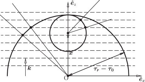
Figure 5: Illustrates that the angular scale of a given comoving $k$-mode subtended on the CMB sky of an observer at high redshift is greater than the angular scale of the same $k$-mode on the CMB sky of an observer at low redshift.

At very low redshift, any cluster will be correlated with any other, and we get back the usual cosmic variance constraint. In other words, we can beat the cosmic variance on $C_{2}(\tau<\tau_{0})$, but not on $C_{2}(\tau_{0})$, today’s quadrupole.

To demonstrate the reduction in cosmic variance, we first combine the $Q$ and $U$ measurements to obtain an improved estimator of $C_{2}(\tau)$. Taking a linear combination of $\widehat{C}^{Q}_{2},\widehat{C}^{U}_{2}$ yields an improved estimator,

$$\widehat{C}^{P}_{2}(\tau) \equiv \alpha\widehat{C}^{Q}_{2}(\tau)+(1-\alpha)\widehat{C}^{U}_{2}(\tau)\ ,$$ (72)

with $0\leq\alpha\leq 1$. This has variance

$$\mbox{Var}\;\widehat{C}^{P}_{2}(\tau) = \alpha^{2}\mbox{Var}\;\widehat{C}^{Q}_{2}(\tau)+(1-\alpha)^{2}\mbox{Var}\;\widehat{C}^{U}_{2}(\tau)$$ (73)

$$\quad\quad+2\alpha(1-\alpha)\;\mbox{Cov}(\widehat{C}^{Q}_{2},\widehat{C}^{U}_{2})\ .$$

It is easy to see that the covariance $\mbox{Cov}(\widehat{C}^{Q}_{2},\widehat{C}^{U}_{2})$ is zero because of the relations in equations (IV), which imply $\mbox{Var}_{2}(Q,U)=0$. Thus the optimum value of $\alpha$ is trivially $\alpha=1/2$.

With these expressions we can compute the variance of our estimator for $C_{2}$ given a set of cluster positions and optical depths $\{\mbox{\boldmath$x$}_{i}\},\;\{\tau_{\rm{C},i}\}$. For simplicity, we will compute here only the variances for sets of clusters which lie on a given redshift shell, distributed in random directions. In the left panel of Fig. 6 we show the variance of the estimator for $C_{2}$ obtained from hypothetical cluster polarization measurements from sets of $10$ and $100$ clusters, all on the same shell of redshift $z$, distributed in random directions on the sky. (We assume the cosmological parameters $\Omega_{m}=0.35,\;\Omega_{\Lambda}=0.65$, power spectral index $n=1$). In the left panel, we show the variance of the estimator for $C_{2}$, as a fraction of $C_{2}$ at $z=0$, from separate sets of clusters confined to redshift shells as a function of the redshift of the shell.

For simplicity we have assumed that all clusters have the same optical depth $\tau_{\rm C}$, so the weights given in equation (67) are all equal, $W_{i}=\tau_{\rm C}^{-2}/N$. The filled squares indicate the square root of $\mbox{Var}\;\widehat{C}^{P}_{2}$, the variance of the average estimator for $C_{2}$, $(\widehat{C}^{Q}_{2}+\widehat{C}^{U}_{2})/2$, for $10$ and $100$ clusters as indicated. This is expressed as a fraction of the Sachs-Wolfe contribution to $C_{2}$, which is independent of redshift for $n=1$. The horizontal dashed line at $\sqrt{2/5}\approx 0.63$ indicates the cosmic variance limit on a single CMB sky given in Eqn. (9). (Note that the ISW contribution is included in these calculations, but omitting it leads to a difference of less than a few percent in the curves in Fig. 6). As $z\rightarrow 0$, the estimator variance slightly exceeds the cosmic variance limit given a single CMB sky — clusters with overlapping correlation spheres as $z\rightarrow 0$ are no more useful than a direct measurement of the quadrupole on our sky by e.g. WMAP. In fact our estimator of $C_{2}$ is worse than a direct measure — but an optimal estimator could be constructed which would yield all of the $a_{2m}$ at $z\approx 0$ from cluster measurements at various points on the sky. As $z\rightarrow\infty$, the estimator variance goes as $\sim 1/\sqrt{N}$ (as $z\rightarrow\infty$, the variance approaches $0.923/\sqrt{N}$. This may be derived by averaging the estimator variances in Eqn. (V) over angles in the $N\rightarrow\infty$ limit).

Thus if we have enough clusters, we can measure $C_{2}(z)$ at increasingly high accuracy as the redshift shell increases. However the fact that $C_{2}(z>0)$ can be measured more accurately than $C_{2}(z=0)$ does not necessarily mean that we can reconstruct the primordial power more accurately than we could using only say the WMAP multipoles, unless the variance in our estimator is less than the variance in the CMB multipole which probes the power at the scale corresponding to the quadrupole at redshift $z$.

In the right panel of Fig. 6 we show the variance of our estimator of $C_{2}$, except divided through by the cosmic variance in the CMB multipole $C_{l_{\rm{eff}}}$, where $l_{\rm{eff}}$ is the $l$-scale on our sky corresponding to the $l=2$ scale on the redshift shell at $z>0$. To be explicit, we are plotting

$$\frac{\sqrt{\mbox{Var}\;\widehat{C}_{2}}}{\sqrt{2/(2l_{\rm{eff}}+1)}\;C_{l_{\rm{eff}}}}\ .$$ (74)

This is the key plot, since if this ratio is less than unity, we have shown that this method can improve on the cosmic variance limits inherent in the existing CMB data, as discussed in the introduction. A reasonable approximation for $l_{\rm{eff}}$ is to take the real $l$ value corresponding to the comoving radius of the last scattering sphere at the redshift $z$, namely $l_{\rm{eff}}=2/(1-\chi/(\tau_{0}-\tau_{r}))$ where $\chi(z)$ is the comoving distance of the shell. Note that there is no one length scale or ($z=0$) harmonic which corresponds to the ($z>0$) quadrupole, since a single angular harmonic mode has power spread over a range of scales. In Appendix B we check the approximation for $l_{\rm{eff}}$ given above by considering the $k$-space window function of the quadrupole, and find that a slight modification to the formula for $l_{\rm{eff}}$ given above gives a better approximation. We use this modified formula in our subsequent calculations. We opt to compute $l_{\rm{eff}}$ as a real number and interpolate between the $C_{l}$’s at the integer values of $l$ bracketing $l_{\rm{eff}}$, to obtain the corresponding cosmic variance. This will give a reasonably good approximation to the accuracy achievable in power spectrum estimation.

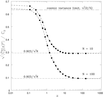
(a)  $\mbox{Var}\;C_{2}(z)$

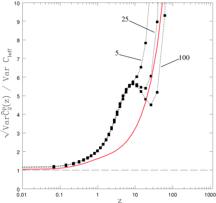
(b)  Ratio of $\mbox{Var}\;C_{2}(z)$ to $\mbox{Var}\;C_{l_{\rm{eff}}}(z)$

Figure 6: Reduction in cosmic variance with clusters distributed on various redshift shells in random directions.

A rough estimate of the maximum number $N_{\mbox{max}}$ of clusters with uncorrelated signals available on a given redshift shell is given by dividing the area of the shell by the area of a circle with radius equal to that of the last scattering sphere at that redshift:

$$N_{\mbox{max}}=1+4\chi^{2}/(\tau_{0}-\tau_{r}-\chi)^{2}\ ,$$ (75)

where $\chi(z)$ is the comoving distance to the shell. The first term is added to allow for the fact that at least one independent cluster signal is available at low redshift. An approximation to the minimum estimator variance achievable on a given redshift shell is then given by:

$$\frac{\sqrt{2/5}\;C_{2}(z=0)}{\sqrt{N_{\mbox{max}}}}\ .$$ (76)

An approximate lower bound on the ratio of the square root of the estimator variance and the cosmic variance in $C_{l_{\rm{eff}}}$ is thus given by:

$$\frac{C_{2}(z=0)}{C_{l_{\rm{eff}}}}\sqrt{\frac{2l_{\rm{eff}}+1}{N_{\mbox{max}}}}\ .$$ (77)

This is shown by the solid curve in the right panel of Fig. 6. Since this curve exceeds $1$ for all values of $z$, this suggests that the cosmic variance is not reducible below the WMAP levels with the cluster technique even without computing the detailed correlations.

In the right panel of Fig. 6, the black squares joined by dashed lines show the ratio (74) computed with the full expression for the estimator variance, plotted for sets of $5$, $25$ and $100$ clusters as indicated. Clearly there is no reduction in variance below the WMAP cosmic variance at any redshift with up to $100$ clusters, as expected from our rough analysis. The three curves are barely distinguishable up to $z\approx 10$, reflecting the fact that at low redshift increasing the number of clusters does not enhance the reduction in cosmic variance since the polarization signals are correlated. Increasing the number of clusters further will not lead to significant improvement, at least with signals from $z<10$. For $z>10$, the $N=25$ and $N=100$ cases begin to show a drop in the ratio, as the redshift shell expands (and last scattering spheres around each cluster shrink) to the point at which the signals from each cluster are uncorrelated. As $z$ increases eventually the ratio in the $N=25$ and $N=100$ cases begins to grow again, since $l_{\rm{eff}}$ is increasing as the last scattering spheres shrink, and so the cosmic variance in $C_{l_{\rm{eff}}}$ is decreasing.

Unfortunately it seems that the cluster technique, at least using the estimator we propose, is not competitive with the CMB data at $z=0$ for estimation of the power at a given scale. In future work it would be interesting to attempt to construct a better estimator — for example combining signals from sets of clusters distributed at arbitrary redshift rather than on redshift shells would presumably lead to some improvement. However we emphasize that this technique is still a useful probe of the time evolution of $C_{2}$, and possibly the ISW effect.

VI Discussion

We have developed a statistical theory of the part of the polarization signal in the CMB in the direction of galaxy clusters produced by scattering of the CMB temperature quadrupole. We have shown explicitly that it is possible to use the indirect information about the last scattering surfaces of distant observers contained in these polarization measurements to constrain the $l=2$ angular power spectrum harmonic of the CMB, $C_{2}$, as a function of redshift with greater statistical accuracy. We also showed however that it not possible to use the cluster polarization measurements to probe the power on a given scale with higher accuracy than the limits imposed by cosmic variance on the single sky CMB data. Thus power spectrum estimation cannot be improved using this method.

But we believe the cluster method is still of considerable value though, since it serves as a probe of the physical mechanism which might have suppressed the quadrupole. It has been noted that the quadrupole seems to be lower than might be expected due to a statistical fluctuation alone (deOliveira-Costa:2003pu, ). The quadrupole may be anomalously low, that is lower than the standard models predict, for various reasons: a cutoff at large scales in the fluctuation power spectrum, different-than-expected behavior of the transfer function at large scales, or effects associated with the large-scale topology or geometry of the universe. There could conceivably be other explanations, but these are the simplest. Signatures of these effects could be present in the time evolution of $C_{2}$. For example if the quadrupole is low because of some topological suppression, we should see a rise in $C_{2}$ with redshift as the scale probed falls below the local quadrupole scale (but if the standard models are correct, there would be no such rise, at least in the $n=1$ case).

One might be worried that since the accuracy of the cluster measurement of $C_{2}$ is not higher than the accuracy of the measurement of the corresponding WMAP harmonic, as shown is §V, the cluster method may not provide any more information that that already contained in the WMAP data. However the cluster technique yields information which is not obtainable with WMAP (about perturbations on last scattering surfaces different to our own) and is thus complementary. In future work it would be desirable to perform a full analysis of the feasibility of using the cluster method to detect the effects of topology (or other quadrupole suppression mechanisms) in the time evolution of $C_{2}$, and a comparison with what we can already learn from the WMAP data.

We also showed that in the standard $\Lambda$CDM model the ISW effect produces a small ($\approx 2$%) bump in CMB harmonic $C_{2}(\tau)$, which is swamped by the high cosmic variance at low redshift even using large numbers of clusters. However the ISW effect produces a significant feature in the two-point correlation function of the Stokes parameters which might be detectable. Detection of the ISW effect would provide additional information about the acceleration of the universe and the dark energy. We also note that this method is a rather sensitive probe of deviations from the scale-invariant power spectrum, because if $n\neq 1$ then the Sachs-Wolfe contribution to $C_{2}(\tau)$ either grows or decays rapidly with conformal time.

The procedure we have outlined is something of an idealization. We assumed that the polarization signal induced by the quadrupole is obtainable from many clusters at the same redshift, and we ignored noise and contamination of the signal. In practice there are contaminating polarization signals from the kinetic and thermal Sunyaev-Zeldovich effects (Diego:2003dp, ), and distortions in the polarization field due to lensing (2000ApJ…538…57S, ). Clearly separating the quadrupole signal from the other contaminants would be a major experimental challenge. However the signal to noise may be increased to some extent by combining signals from clusters located at similar directions and redshifts, since the signal from sufficiently nearby clusters is strongly correlated. It remains to be seen if this technique will be a practically useful cosmological probe.

Appendix A Transfer equation for polarization matrix

We found it convenient to write the transfer equation for generation of polarization by Thomson scattering in matrix form. This approach is similar to the “density matrix” formalism for polarized radiation transfer (1994PhDT……..24K, ; 2000PhRvD..62d3004C, ).

The transfer equation is usually written in terms of the Stokes parameters, which are time averages of quadratic products of the complex amplitudes of the electric field components $E_{i}$ of the electromagnetic wave. The polarization state and intensity of a beam of light propagating in the $z$–direction is characterized completely by the $2\times 2$ Hermitian matrix $\langle E_{i}E^{*}_{j}\rangle$, with $(i,j)\in\{x,y\}$ (the brackets denote a time average). An obvious generalization is to allow $(i,j)$ to become Cartesian tensor indices and to run over all of $\{x,y,z\}$. We obtain a $3\times 3$ polarization matrix associated with photon direction $\bm{n}$:

$$Q_{ij}(\bm{n})=\left<E_{i}E_{j}^{*}\right>\ .\quad\quad(i,j)\in\{x,y,z\}$$ (78)

With this matrix we are no longer restricted to considering a beam propagating along a coordinate axis. For a given photon direction $\bm{n}$, the electric fields are transverse to $\bm{n}$, implying

$$n^{i}Q_{ij}(\bm{n})=0\ .$$ (79)

Consider now a superposition of beams of various directions $\bm{n}$ and momenta $\bm{p}=p\bm{n}$, where $p$ is the frequency (we set $c=h=1$ for convenience). In this case, $Q_{ij}$ cannot be considered a function of the photon momenta, but an intensity matrix can be defined associated with each photon direction and frequency. Recall from the definition of specific intensity that the energy density is given by $Q^{i}_{i}=\int I(\bm{p})\,dp\,d\Omega$, where $I(\bm{p})$ is the specific intensity and $d\Omega$ is the solid angle element associated with the photon direction $\bm{n}$. Similarly we can express each element of the matrix $Q_{ij}$ in terms of specific intensity matrices $I_{ij}$:

$$Q_{ij}=\int dp\;d\Omega\;I_{ij}(\bm{p})\ .$$ (80)

Now the Stokes parameters are defined with respect to a particular choice of “polarization basis”. This is a pair of mutually orthogonal unit vectors $\bm{\epsilon}^{(1)},\bm{\epsilon}^{(2)}$, both orthogonal to the beam direction. The Stokes parameters are given in terms of $I_{ij}$ and the polarization basis vectors as:

$$\frac{I+Q}{2} = \epsilon^{(1)}_{i}\epsilon^{(1)}_{j}I_{ij}\ ,$$

$$\frac{I-Q}{2} = \epsilon^{(2)}_{i}\epsilon^{(2)}_{j}I_{ij}\ ,$$

$$\frac{U+iV}{2} = \epsilon^{(1)}_{i}\epsilon^{(2)}_{j}I_{ij}\ ,$$

$$\frac{U-iV}{2} = \epsilon^{(2)}_{i}\epsilon^{(1)}_{j}I_{ij}\ .$$ (81)

In the case of a beam propagating in the $z$-direction for example, we have, choosing polarization basis vectors $\bm{\epsilon}^{(1)}=\bm{x},\;\bm{\epsilon}^{(2)}=\bm{y}$,

$$I_{ij}=\frac{1}{2}\left(\begin{array}[]{ccc}I+Q&U+iV&0\\ U-iV&I-Q&0\\ 0&0&0\end{array}\right)\ .$$ (82)

The matrix is non-zero only in the two dimensional subspace spanned by $\bm{\epsilon}^{(1)},\bm{\epsilon}^{(2)}$.

We need to construct the matrix of an unpolarized beam propagating in a general direction $\bm{n}$. The only quantities available to form this matrix are the intensity $I$, the components of the direction vector $\bm{n}$, and the Kronecker delta $\delta_{ij}$. The matrix must therefore be of the form:

$$I_{ij}(\bm{n})=A\delta_{ij}+Bn_{i}n_{j}\ .$$ (83)

The matrix of an unpolarized beam propagating in the $z$–direction is obviously

$$I_{ij}=\frac{I}{2}\left(\begin{array}[]{ccc}1&0&0\\ 0&1&0\\ 0&0&0\end{array}\right).$$ (84)

Comparing this with the form of Eqn. (83) for the special case $n_{i}=\delta_{iz}$, we see that $A=-B=I/2$. Thus the matrix of an unpolarized beam in a general direction $\bm{n}$ is

$$I_{ij}(\bm{n})=\frac{I}{2}(\delta_{ij}-n_{i}n_{j})\ .$$ (85)

The polarization magnitude of the beam described by a general matrix $I_{ij}$ is given by

$$\Pi^{2}=2\mbox{Tr}[\bm{I}^{2}]/\mbox{Tr}[\bm{I}]-1\ ,$$ (86)

which may be readily checked with the matrix (82).

We now derive the equation for the time evolution of the polarization matrix due to Thomson scattering from a distribution of stationary electrons. For a completely linearly polarized beam, $Q^{ij}\epsilon^{\ast}_{i}\epsilon_{j}$ is the time-average energy density for electromagnetic radiation of polarization $\bm{\epsilon}$, where $\bm{\epsilon}\cdot\bm{\epsilon}=1$. Consider a completely polarized beam with polarization vector $\bm{\epsilon}$ and momentum $\bm{p}=p\bm{n}$ incident upon an electron at rest The polarization matrix of the incident beam is $Q_{ij}=Q\epsilon_{i}\epsilon_{j}^{\ast}$ where $cQ$ is the incident flux (we choose units such that $c=1$). Normalization of the polarization vector implies $Q=Q_{ij}\epsilon^{\ast}_{i}\epsilon_{j}$. In the Thomson limit, in which the electron recoil is negligible, the differential cross section for Thomson scattering of a beam into final momentum $\bm{p}^{\prime}=p^{\prime}\bm{n}^{\prime}$ and polarization $\bm{\epsilon}^{\prime}$ is (Jackson, )

$$\frac{d\sigma}{d\Omega^{\prime}}=\frac{3\sigma_{\rm T}}{8\pi}\left|\bm{\epsilon}^{\ast}\cdot\bm{\epsilon}^{\prime}\right|^{2}\ .$$ (87)

where $d\Omega^{\prime}$ is the solid angle element associated with the scattered photon direction $\bm{n}^{\prime}$. Thus the power per unit solid angle in the scattered beam is

$${dP^{\prime}\over d\Omega^{\prime}}={3\sigma_{\rm T}\over 8\pi}\,Q\left|\bm{\epsilon}^{\ast}\cdot\bm{\epsilon}^{\prime}\right|^{2}\ .$$ (88)

We may also write $Q|\bm{\epsilon}^{\ast}\cdot\bm{\epsilon}^{\prime}|^{2}=Q_{ij}\epsilon^{\prime\ast}_{i}\epsilon^{\prime}_{j}$.

Next consider a gas of electrons all at rest with number density $n_{e}$. We can ignore the thermal motion of the electrons here since the correction to the polarization due to a finite electron temperature $T_{e}$ will be down by a factor of $\theta_{e}\equiv k_{B}T_{e}/m_{e}c^{2}$. At cluster temperatures $\theta_{e}\approx 0.01$, so we may assume stationary electrons. Assuming incoherent scattering, multiplying Eqn. (88) by $n_{e}d\Omega^{\prime}$ converts scattered power per electron to the rate of change of energy density in final polarization state $\bm{\epsilon}^{\prime}$:

$${dQ^{\prime}_{ij}\over dt}\,\epsilon^{\prime\ast}_{i}\epsilon^{\prime}_{j}={3\sigma_{\rm T}\over 8\pi}n_{e}Q_{ij}\epsilon^{\prime\ast}_{i}\epsilon^{\prime}_{j}\,d\Omega^{\prime}\ ,$$ (89)

where $Q^{\prime}_{ij}$ is the polarization matrix of the scattered beam. Using equation (80), setting $p=p^{\prime}$ since we are working in the Thomson limit, and assuming the incident beam is monochromatic, we find

$${dI^{\prime}_{ij}\over dt}\,\epsilon^{\prime\ast}_{i}\epsilon^{\prime}_{j}={3\sigma_{\rm T}\over 8\pi}n_{e}\,\epsilon^{\prime\ast}_{i}\epsilon^{\prime}_{j}\int d\Omega\;I_{ij}\ ,$$ (90)

where $d\Omega$ is the solid angle element associated with the incident photon direction $\bm{n}$. Note that this equation is valid now for an arbitrary incident radiation field.

We cannot now just remove the polarization factors and conclude $dI^{\prime}_{ij}\propto\int d\Omega\,I_{ij}$ because the polarization of the incoming wave does not lie in the same plane as the polarization of the scattered wave. For a given outgoing momentum $\bm{p}^{\prime}$, the outgoing polarization is a linear combination of two basis vectors $\bm{\epsilon}^{\prime}_{1}$ and $\bm{\epsilon}^{\prime}_{2}$ (orthonormal and orthogonal to the photon momentum $\bm{p}^{\prime}$). Thus, $I_{ij}\epsilon^{\prime\ast}_{i}\epsilon^{\prime}_{j}$ projects out of the incoming matrix $I_{ij}$ only those components lying in the $\bm{\epsilon}^{\prime}_{1}$-$\bm{\epsilon}^{\prime}_{2}$ plane. This projection is equivalent to first projecting $I_{ij}$ with $\bm{\epsilon}^{\prime}_{1}\otimes\bm{\epsilon}^{\prime}_{1}+\bm{\epsilon}^{\prime}_{2}\otimes\bm{\epsilon}^{\prime}_{2}$. This is equivalent to projecting out the unphysical components by acting with the matrix

$$P_{ij}(\bm{n^{\prime}})\equiv\delta_{ij}-n^{\prime}_{i}n^{\prime}_{j}\ .$$ (91)

Projecting the final polarization vector with $P_{ij}(\bm{n}^{\prime})$ does not change it: $P_{ij}(\bm{n}^{\prime})\epsilon^{\prime}_{j}=\epsilon^{\prime}_{i}$. It follows that $I_{ij}(\bm{n})\epsilon^{\prime\ast}_{i}\epsilon_{j}=I_{kl}(\bm{n})P_{ik}(\bm{n}^{\prime})P_{jl}(\bm{n}^{\prime})\epsilon^{\prime\ast}_{i}\epsilon_{j}$. Now it is safe to remove the outgoing polarization vectors from Eqn. (90).

We conclude that, for any initial and final polarizations,

$${dI^{\prime}_{ij}(\bm{n}^{\prime})\over dt}={3\sigma_{\rm T}\over 8\pi}n_{e}P_{ik}(\bm{n}^{\prime})\;P_{jl}(\bm{n}^{\prime})\int d\Omega\;I_{kl}(\bm{n})\ .$$ (92)

This is the equation we need. The projection tensors are easy to understand: the scattered matrix is simply proportional to the incident matrix after the unphysical polarization components (those proportional to $\bm{n}^{\prime}$) are eliminated.

If the integration time is sufficiently short, we may replace $n_{e}\sigma_{\rm T}\,dt$ with the optical depth to Thomson scattering, $\tau_{\rm C}$. Then we have for the polarization matrix of the scattered radiation field:

$$I^{\prime}_{ij}(\bm{n}^{\prime})={3\tau_{\rm C}\over 8\pi}P_{ik}(\bm{n}^{\prime})\;P_{jl}(\bm{n}^{\prime})\int d\Omega\;I_{kl}(\bm{n})\ .$$ (93)

If the incoming radiation field is assumed to be unpolarized, then the incident matrix has the form of Eqn. (85) and we may set $I_{kl}(\bm{n})=I(\bm{n})\;P_{kl}(\bm{n})/2$. Thus

$$I^{\prime}_{ij}(\bm{n}^{\prime})={3\tau_{\rm C}\over 16\pi}P_{ik}(\bm{n}^{\prime})\;P_{jl}(\bm{n}^{\prime})\int d\Omega\;I(\bm{n})\;P_{kl}(\bm{n})\ .$$ (94)

This is the form of the transfer equation used in Eqn. (44).

Note that this is not the full transfer equation, since we have ignored the effect of scattering out of the beam direction. But here we are only interested in the polarization generated by scattering into the observation direction, and the loss of photons from the beam only affects this at $O(\tau_{\rm C}^{2})$.

Assuming a blackbody spectrum of incident photons, this transfer equation also holds for the brightness temperature polarization matrix (since Thomson scattering does not change the photon frequency, and there is no Doppler shift because we have assumed the electrons are stationary, thus the scattered radiation field also has a blackbody spectrum). We may suppress the frequency dependence of the (brightness temperature) polarization matrix and associated Stokes parameters of the scattered photon also, since there is no energy transfer.

Appendix B Effective scale of the $z>0$ quadrupole

Figure 7: The lower, middle, and upper sets of points indicate the wavenumbers at the 20th, 50th and 80th percentile respectively of the window function for the $l=2$ harmonic, as a function of redshift. This gives the range of wavenumbers contributing to the CMB quadrupole at a given redshift. The lower line shows the estimated wavenumber $k_{\rm{eff}}$ corresponding to the radius of the last scattering sphere. The upper line shows $k^{\prime}_{\rm{eff}}=3.12\;k_{\rm{eff}}$, which better matches the median of the window function.

The $l=2$ harmonic of the CMB anisotropy at redshift $z=0$ contains contributions from a broad range of wavenumbers of order $c/H_{0}$. At higher redshifts the CMB quadrupole probes the potential on a smaller last scattering surface than at redshift $z=0$. In §V we need to associate the quadrupole at $z>0$ to an effective angular harmonic mode $l_{\rm{eff}}$ probing roughly the same angular scales on the $z=0$ sky. This is most easily done by finding the comoving wavenumber $k_{\rm{eff}}$ which best approximates the scale probed by the quadrupole on the $z>0$ last scattering sphere, and setting $l_{\rm{eff}}=2\;k_{\rm{eff}}/k_{0}$ where $k_{0}$ is an estimate of the scale probe by the quadrupole at $z=0$. We take $k_{0}=1/(\tau_{0}-\tau_{r})$ (we have set $c=1$).

An approximation to the effective length scale probed by the CMB quadrupole at a given redshift is given by the radius of the last scattering sphere at that redshift, $r=(\tau_{0}-\tau_{r})-\chi$ (where $\chi(z)$ is the comoving distance to redshift $z$). With $k_{\rm{eff}}=1/r$ this gives $l_{\rm{eff}}=2/(1-\chi/(\tau_{0}-\tau_{r}))$.

To check this approximation, there is a useful method (2002PhRvD..66j3508T, ) which yields an estimate of the range of wavenumbers $k$ which contribute to each $l$ mode. The procedure is to first find the following window function:

$$\mathcal{P}(k|\tau,l)=\frac{(4\pi)^{2}\Delta^{2}_{l}(k,\tau)P_{\phi}(k)\;k^{3}}{C_{l}(\tau)},\;\;\;\;\;\;\;\;\int_{-\infty}^{\infty}\mathcal{P}(k|\tau,l)\;d\ln k=1\ ,$$ (95)

where the transfer function is computed with some assumed model. In the $l=2$ case the Sachs-Wolfe transfer function is sufficient until we consider rather high redshifts. The $k$ scale probed by this harmonic is then taken to be the median $k_{i}$ of the window function. The range of wavenumbers contributing to the $l$ harmonic at a given redshift is indicated by the $20$th to the $80$th percentile of the window function (which corresponds to full-width-half-maximum in the Gaussian case). The $l=2$ case is shown by the points in Fig. 7. For comparison the estimate $k_{\rm{eff}}$ is shown by the lower line. In fact we obtain a much better match to the median window function estimate with the wavenumber $k^{\prime}_{\rm{eff}}=3.12\;k_{\rm{eff}}$, as shown by the upper line. We therefore use the following modified approximation for the effective angular harmonic mode in the calculations in §V: $l^{\prime}_{\rm{eff}}=6.24/(1-\chi/(\tau_{0}-\tau_{r}))$.

References

(1)
M. Kamionkowski and A. Loeb, Phys. Rev. D56, 4511 (1997).
(2)
A. Cooray and D. Baumann, Phys. Rev. D67, 63505 (2003).
(3)
N. Seto and M. Sasaki, Phys. Rev. D62, 123004 (2000).
(4)
A. Kosowsky, Annals of Phys. 246, 49 (1996).
(5)
A. Challinor, Phys. Rev. D62, 43004 (2000).
(6)
C. Ma and E. Bertschinger, ApJ 455, 7 (1995).
(7)
J. A. Peacock, Cosmological physics (Cambridge University Press, UK,
1999).
(8)
M. E. Rose, Elementary Theory Of Angular Momentum (Dover, New York,
1995).
(9)
R. K. Sachs and A. M. Wolfe, ApJ 147, 73 (1967).
(10)
U. Seljak and M. Zaldarriaga, ApJ 469, 437 (1996).
(11)
S. Bashinsky and E. Bertschinger, Phys. Rev. D65, 123008 (2002).
(12)
T. Padmanabhan, Theoretical Astrophysics. Volume III: Galaxies and
Cosmology (Cambridge University Press, UK, 2003).
(13)
S. Dodelson and J. M. Jubas, ApJ 439, 503 (1995).
(14)
D. J. Heath], MNRAS 179, 351 (1977).
(15)
A. Challinor and F. van Leeuwen, Phys. Rev. D65, 103001 (2002).
(16)
F. Byron and R. Fuller, Mathematics of Classical and Quantum
Physics (Dover, New York, 1992).
(17)
W. Hu and M. White, Phys. Rev. D56, 596 (1997).
(18)
A. de Oliveira-Costa, M. Tegmark, M. Zaldarriaga, and A. Hamilton, Phys. Rev.
D69, 063516 (2004).
(19)
J. M. Diego, P. Mazzotta, and J. Silk, Astrophys. J. 597, L1 (2003).
(20)
U. Seljak and M. Zaldarriaga, ApJ 538, 57 (2000).
(21)
J. D. Jackson, Classical Electrodynamics, 3rd Ed. (Wiley, New
York, 1998).
(22)
M. Tegmark and M. Zaldarriaga, Phys. Rev. D66, 103508 (2002).