The spacetime associated with galactic dark matter halos.

Abstract

We show how an adequate post–Newtonian generalization can be obtained for Newtonian dark matter halos associated with an empiric density profile. Applying this approach to halos that follow from the well known numerical simulations of Navarro, Frenk and White (NFW), we derive all dynamical variables and show that NFW halos approximatelly follow an ideal gas type of equation of state which fits very well to a polytropic relation in the region outside the core. This fact suggests that “outer” regions of NFW halos might be related to equilibrium states in the non–extensive Statistical Mechanics formalism proposed by Tsallis.

I Introduction

The issue of dark matter clustering in halos of virialized galactic structures is one of the most interesting open problems in astrophysics and cosmology KoTu ; Padma1 ; Peac ; Ellis ; Fornengo . The physical properties of this dark matter are uncertain, leading to various proposed physical matter models: thermal sources, meaning a colissionless gas of weakly interacting massive particles (WIMP’s), which can be very massive ($m\sim 100-200$ GeV) supersymmetric Ellis (“cold dark matter” CDM) or self–interacting less massive ($m\sim$ KeV) particles scdm ; wdm (“warm” DM). Other proposals include scalar fields (real and complex) sfe_1 ; sfe_2 , global momopoles sfe_3 , axions, etc. However, all these models must comply from inferred direct and indirect observations that reveal the presence of DM: velocity profiles of rotating stars, microlensing and tidal effects affecting satelite galaxies and galaxies within galactic clusters. Galactic DM is mixed with visible baryonic matter (stars and gas) clustering in galactic disks, making up about 5–10 % of the total galactic mass. Hence, it is a good approximation to identify the gravitational field of a galaxy with that of its DM halo, considering visible matter as “test particles” in this field HGDM ; Lake .

Realistic galactic halos are obviously not spherically symmetric, but they are approximatelly so, since their global rotation is not dynamically significant urc . Hence, we will consider throughout this paper that halos are spherically symmetric equilibrium configurations. Assuming the CDM paradigm and spherical symmetry, we can distinguish two types of halo models: those obtained from a Kinetic Theory approach, whether based on specific theoretical considerations or on convenient ansatzes that fix a distribution function satisfying Vlassov’s equation BT , or those emerging from “universal” density profiles obtained empirically by N–body numerical simmulations nbody_1 ; nbody_2 ; nbody_3 . In this paper we will consider the latter apprach, based on the well known numerical simulations of Navarro, Frenk and White (NFW) nbody_1 ; LoMa . Although these simulations yield virialized equilibrium structures that reasonably fit CDM structures at a cosmological scale ($\gtrsim 100$ Mpc), some of their predictions in smaller scales (“cuspy” density profiles and excess substructure) seem to be at odds with observations cdm_problems_1 ; cdm_problems_2 , especially those based on galaxies with low surface brightness (LSB), which are supposed to be overwhelmingly dominated by DM and so well suited to examine the predictions of various DM models.

Galactic halos are newtonian systems characterized by typical velocities, ranging from $5-10$ km/sec for dwarf galaxies up to about $1000-3000$ km/sec for rich clusters. However, we believe that a study of these systems under General Relativity, as a post–Newtonian approximation, might provide new information that can be useful and interesting for gravitational lensing and for the study of the interplay between cosmological scale evolution and galactic DM. In any case, since General Relativity is the best available theory of classical gravity, it is relevant from a theoretical point of view to be able to construct spacetimes that are suitable for important self–gravitating structures like galactic halos.

All DM halo models derive a full set of dynamical variables from a given “mass–density” profile. In a post–newtonian relativistic generalization we will assume that this density is the dominant rest–mass contribution to the matter–energy density, made up by rest–mass and an internal energy term proportional to suitably defined temperature and pressure (of a kinetic nature). Thus, we will assume an “ideal gas” type of equation of state RKT ; Padma2 ; Padma3 in which this internal energy density becomes determined only by the hydrostatic equations themselves in the case of isotropic velocity distributions. In the anistropic case, which we leave for a future paper enproceso , various empirical ansatzes can be assumed in order to relate radial and angular components of the stress tensor.

II Newtonian NFW galactic halos.

Following the CDM paradigm and assuming spherical symmetry, galactic halos must satisfy the following Newtonian equations of hydrostatic equilibrium

$$M\,^{\prime}=4\,\pi\,\rho\,r^{2},$$ (1)

$$\Phi\,^{\prime}=\frac{4\,\pi\,GM}{r^{2}},$$ (2)

as well as the Navier–Stokes equation

$$P\,^{\prime}=-\rho\,\Phi\,^{\prime}-\frac{2\,\alpha}{r}\,P,$$ (3)

where $P$ is the “radial” pressure and

$$\alpha=\frac{P-P_{\perp}}{P},$$ (4)

is the anisotropy factor relating $P$ with the tangential pressure $P_{\perp}$. Since we have three equations for five unknowns ($\rho,\,M,\,\Phi,\,P,\,\alpha$), this system can be made determined if two of these five functions becomes specified, for example, by assuming an “equation of state” somehow relating $P$ and $P_{\perp}$ with $\rho$. In the case of N–body numerical simmulations, we have virialized structures whose density profile $\rho=\rho(r)$ can be approximately fit to a “universal” empirical function urc ; nbody_1 ; LoMa . The Newtonian system (1)–(4) becomes determined once we have this density profile together with a suitable expression for $\alpha$. In general, the simmulations yield anisotropic velocity distributions, so that specific ansatzes can be assumed or prescribed OM for $\alpha\neq 0$.

The well known N–body numerical simmulations by Navarro, Frenk and White (NFW) yield the following “universal” expression for the density profile of virialized galactic halo structures nbody_1 ; LoMa :

$$\rho_{{}_{\mathrm{NFW}}}=\frac{\delta_{0}\,\rho_{0}}{x\,\left(1+x\right)^{2}},$$ (5)

where

$$\delta_{0} = \frac{\Delta\,c_{0}^{3}}{3\left[\ln\,(1+c_{0})-c_{0}/(1+c_{0})\right]},$$ (6)

$$\rho_{0} = \rho_{\mathrm{crit}}\,\Omega_{0}\,h^{2}=253.8\,h^{2}\,\Omega_{0}\,\frac{M_{\odot}}{\text{kpc}^{3}},$$ (7)

$$x = \frac{r}{r_{s}},\qquad r_{s}=\frac{r_{\textrm{\tiny{vir}}}}{c_{0}},$$ (8)

The virial radius $r_{\textrm{\tiny{vir}}}$ is given in terms of the virial mass $M_{\textrm{\tiny{vir}}}$ by the condition that average halo density equals $\Delta$ times the cosmological density $\rho_{0}$ Padma1

$$\Delta\,\rho_{0}=\frac{4\,\pi\,M_{\textrm{\tiny{vir}}}}{3\,r_{\textrm{\tiny{vir}}}^{3}},$$ (9)

where $\Delta$ is a model–dependent numerical factor (for a $\Lambda$CDM model with total $\Omega_{0}=1$ we have $\Delta\sim 100$ LoHo ). The concentration parameter $c_{0}$ can be expressed in terms of $M_{\textrm{\tiny{vir}}}$ by c0

$$c_{0}=62.1\times\left(\frac{M_{\textrm{\tiny{vir}}}\,h}{M_{\odot}}\right)^{-0.06}\,\left(1+\epsilon\right),$$ (10)

where $-0.5\lesssim\epsilon\lesssim 0.5$. Hence all quantities depend on a single free parameter $M_{\textrm{\tiny{vir}}}$ with a dispersion range given by $\epsilon$ for different halo concentrations. The NFW mass function and Newtonian potential follow from integrating (1) and (2) for $\rho$ given by (5)

$$M_{\textrm{\tiny{NFW}}} = 4\,\pi\,r_{s}^{3}\,\delta_{0}\,\rho_{0}\,\left[\ln(1+x)-\frac{x}{1+x}\right],$$ (11)

$$\Phi_{\textrm{\tiny{NFW}}} = -V_{0}^{2}\,\frac{\ln(1+x)}{x}$$ (12)

complying with the boundary conditions

$$M_{\textrm{\tiny{NFW}}}(0) = 0,\qquad M_{\textrm{\tiny{NFW}}}(r_{\textrm{\tiny{vir}}})=M_{\textrm{\tiny{vir}}},$$ (13)

$$-\Phi_{\textrm{\tiny{NFW}}}(0) = V_{0}^{2}\ =\ 4\,\pi\,G\,\delta_{0}\,\rho_{0}\,r_{s}^{2},$$ (14)

while circular rotation velocity (normalized by the characteristic velocity $V_{0}^{2}$) is simply

$$V_{\textrm{\tiny{rot}}}^{2}=r\,\Phi^{\prime}=\frac{4\pi GM}{r}=V_{0}^{2}\left[\frac{\ln(1+x)}{x}-\frac{1}{1+x}\right].$$ (15)

Given $\rho_{\textrm{\tiny{NFW}}},\,M_{\textrm{\tiny{NFW}}}$ and $\Phi_{\textrm{\tiny{NFW}}}$, radial and tangential pressures follow from integrating (3) for a specific choice of $\alpha$. There are analytic solutions of (3) for $\alpha=0$ (isotropic case) and for various empiric expressions for $\alpha$. A thorugh Newtonian treatement of NFW halos is found in LoMa

Notice that according to the density profile (5) we have a diverging density at the symmetry center ($x=0$). This is obviously an unphysical feature and points out to the fact that (5) has not been derived from any theoretical argumentation, but is simply a convenient empirical formula that fits the outcome of the NFW numerical simulations which show that $\rho_{\textrm{\tiny{NFW}}}\propto 1/x$ near the central halo region. Since the virial radius $r_{\textrm{\tiny{vir}}}$ is the physical size of the resulting halos and these simulations are unable to provide adequate resolution for distances to the halo center smaller than approximately 1% of the virial radius NSres , all halo quantities presented here are, strictly speaking, only valid between a minimal $r\sim 0.01\,r_{\textrm{\tiny{vir}}}$ and $r_{\textrm{\tiny{vir}}}$ (see section VII for further discussion on this issue).

III The spacetimes of galactic halos

As a good approximation otro , we can consider the metric of a galactic halo to be given by a suitable “weak field” limit of the spherically symmetric static line element

$$\textrm{d}s^{2}\ =\ -\exp\left(\frac{\Phi}{c^{2}}\right)\,c^{2}\,\textrm{d}t^{2}+\frac{\textrm{d}r^{2}}{1-\kappa_{0}\,M/r},$$

$$+r^{2}(\textrm{d}\theta^{2}+\sin^{2}\theta\textrm{d}\phi^{2}),$$ (16)

where $\Phi(r)$ is the relativistic generalization of the Newtonian gravitational potential and $\kappa_{0}=2G/c^{2}$, so that $M(r)$ has mass units. We will assume a momentum–energy tensor of the form

$$T^{ab}=\ \mu\,u^{a}\,u^{b}+p\,h^{ab}+\Pi^{ab},$$ (17)

where $u^{a}=\exp(-\Phi/c^{2})\,\delta^{a}\,_{t}$,  $h^{ab}=g^{ab}+u^{a}\,u^{b}$ and $\Pi^{ab}$ is the anisotropic and traceless ($\Pi^{a}\,_{a}=0$) stress tensor, which for the metric (16) takes the form

$$\Pi^{a}\,_{b}\ =\ \textbf{diag}\,[0,\,-2\Pi,\,\Pi,\,\Pi]$$ (18)

so that $p$ and $\Pi$ relate to $P$ and $P_{\perp}$ by

$$P_{\perp}-P\ =\ 3\,\Pi,\qquad 2\,P_{\perp}+P\ =\ 3\,p.$$ (19)

The field equations and momentum balance ($T^{ab}\,_{;b}=0$) associated with (16)-(19) are

$$M\,^{\prime} =\ 4\,\pi\,\mu\,r^{2}/c^{2},$$ (20)

$$\Phi\,^{\prime} =\ \frac{\kappa_{0}\,c^{2}}{2}\,\frac{M+4\,\pi\,P\,r^{3}/c^{2}}{r\,(r-\kappa_{0}\,M)},$$ (21)

$$P\,^{\prime} =\ -(\mu+P)\,\frac{\Phi\,^{\prime}}{c^{2}}-\frac{2\,\alpha}{r}\,P,$$ (22)

where $\alpha$ is given by (4). These equations are the relativistic generalization of (1)–(3), though we must provide a relation between $\mu$ and $\rho$. Since the particles in the collisionless gas making up galactic halos are interacting very weakly and the velocity anisotropies tend to be small: $0\leq\alpha\lesssim 0.2$ LoMa , it is reasonable to assume that it is nearly an ideal gas and that total matter–energy density, $\mu$, is the sum of a dominant contribution from rest–mass density, $\rho\,c^{2}$, and an internal energy term that is proportional to the pressure $P$ and to the velocity dispersion $\sigma^{2}=\langle v^{2}\rangle\simeq\langle v_{\perp}^{2}\rangle$. Hence it is reasonable to assume the equation of state of a non–relativistic (but non–Newtonian) ideal gas RKT

$$\mu\ =\ \rho\,c^{2}\,\left[1+\frac{3}{2}\,\frac{\sigma^{2}}{c^{2}}\right],\qquad P\ =\ \rho\,\sigma^{2},$$ (23)

where the velocity dispersion is related to a kinetic temperature $T$ by

$$\sigma^{2}\ =\ \frac{P}{\rho}\ =\ \frac{k_{{}_{B}}\,T}{m},$$ (24)

Since characteristic velocities in galactic halos are Newtonian, we have $\sigma^{2}/c^{2}\ll 1$ and $\mu\approx\rho\,c^{2}$ and so $P\simeq P_{\perp}\ll\rho\,c^{2}$, so that (23) provides a plausible equation of state for a relativistic generalization of galactic halos. It is evident also that in the newtonian limit $\sigma^{2}/c^{2}\ll 1$ we recover the equilibrium equations (1)–(3).

What needs to be done now is to insert the equation of state (23) into the field equations (20)–(22), which becomes a set of equations that, just like (1)–(3), becomes determined once we specify the functional relation $\rho=\rho(r)$ or $\rho=\rho(\Phi)$ and $\alpha(r)$. However, we do not need all the three equations (20)–(22), since numerical simulations yield the density profile (5), we will assume

$$\rho(r)\ =\ \rho_{\textrm{\tiny{NFW}}}(r)$$ (25)

and eliminate $\Phi^{\prime}$ from (21) and (22), leading to the following set:

$$M\,^{\prime} =\ 4\,\pi\,\left[\,\rho_{\textrm{\tiny{NFW}}}+\frac{3}{2}\,\frac{P}{c^{2}}\right]r^{2},$$ (26)

$$P\,^{\prime} =\ -\frac{\kappa_{0}c^{2}}{2}\,\frac{[\rho_{\textrm{\tiny{NFW}}}+\frac{5}{2}P/c^{2}]\,\,[M+4\,\pi\,P\,r^{3}/c^{2}]}{r\,(r-\kappa_{0}\,M)}$$ (27)

$$\quad\ -\frac{2\,\alpha}{r}\,P,$$

which becomes fully determined once we know $\alpha(r)$. We will solve these equations in a post–Newtonian approximation by keeping only terms up to order $\sigma^{2}/c^{2}$. The velocity dispersion $\sigma$ (and/or $T$) can be obtained afterwards from $P$ through (23) and (24).

As mentioned before, we have $\rho_{\textrm{\tiny{NFW}}}\to\infty$ as $x\to 0$. A quick calculation of the Ricci scalar using (21), (26) and (27)

$$R\ =\ \frac{8\pi G}{c^{4}}\,\left[\rho_{\textrm{\tiny{NFW}}}\,c^{2}+\left(2\,\alpha-\frac{3}{2}\right)\,P\right],$$ (28)

reveals the existence of a curvature singularity as $r\to 0$. This is wholy unphysical, since NFW halos within a general relativistic treatment should be weak field static spacetimes. However, as mentioned in the last parragraph of section II, all variables associated with NFW simulations are valid in the range $0.01\lesssim r/r_{\textrm{\tiny{vir}}}\leq 1$. In section VII we discuss how this issue can be dealt with appropriately.

IV Post–Newtonian equations for NFW halos.

It is convenient to work with the following adimensional variables

$$Y =\ \frac{\rho_{\textrm{\tiny{NFW}}}}{\delta_{0}\,\rho_{0}}\ =\ \frac{1}{x\,[1+x]^{2}},$$ (29)

$${\cal{M}} =\ \frac{M}{4\,\pi\,\delta_{0}\,\rho_{0}\,r_{s}^{3}}\ =\ \frac{c_{0}^{3}\,\Delta\,M}{3\,\delta_{0}\,M_{\textrm{\tiny{vir}}}},$$ (30)

$${\cal{P}} =\ \frac{P}{\delta_{0}\,\rho_{0}\,V_{0}^{2}},$$ (31)

where the structural parameters $\delta_{0},\,\rho_{0},\,c_{0},\,\Delta$ and $V_{0}^{2}$ have been introduced in section II. The field equations (26)–(27) now becomes

$$\frac{\textrm{d}{\cal{M}}}{\textrm{d}x} =\ \left[Y+\frac{3}{2}\,\varepsilon\,{\cal{P}}\right]\,x^{2},$$ (32)

$$\frac{\textrm{d}{\cal{P}}}{\textrm{d}x} =\ -\frac{\left[Y+\frac{5}{2}\,\varepsilon\,{\cal{P}}\right]\,\left[{\cal{M}}+\varepsilon\,{\cal{P}}\,x^{3}\right]}{x\,\left[x-2\,\varepsilon\,{\cal{M}}\right]}+\frac{2\alpha}{x}\,{\cal{P}},$$

where

$$\varepsilon\ =\ \frac{V_{0}^{2}}{c^{2}},$$ (34)

so that in the limit $\varepsilon\to 0$ we recover the Newtonian equations (1), (2) and (3). The system (32)–(LABEL:Px) can be integrated by demanding that ${\cal{M}}$ and ${\cal{P}}$ comply with appropriate boundary and initial conditions. Since we have to use the explicit form of $Y$ in (29), then the analytic or numerical solutions of (32)–(LABEL:Px) for specific choices of $\alpha$, boundary conditions depend on $M_{\textrm{\tiny{vir}}}$ through the definitions (6) and (10).

The metric function $M=V_{0}^{2}\,r_{s}\,{\cal{M}}$ follows from (32), while $\Phi$ can be obtained by integrating

$$\frac{\textrm{d}}{\textrm{d}y}\,\left(\frac{\Phi}{V_{0}^{2}}\right)\ =\ \frac{{\cal{M}}+\varepsilon\,{\cal{P}}\,y^{3}}{y\,[y-2\,\varepsilon\,{\cal{M}}]}.$$ (35)

The relativistic generalization of the Newtonian rotation velocity profile are the velocities of test observers along circular geodesics. From sfe_1 ; sfe_2 ; HGDM , these velocities are $V_{\textrm{\tiny{rot}}}^{2}=r\,\Phi^{\prime}$, which in terms of the adimensional variables becomes

$$\frac{V_{\textrm{\tiny{rot}}}^{2}}{V_{0}^{2}}\ =\ \frac{{\cal{M}}+\varepsilon\,{\cal{P}}\,y^{3}}{y-2\,\varepsilon\,{\cal{M}}},$$ (36)

Since $V_{0}$ for typical galactic halos ranges from a few km/sec to $\sim 3000$ km/sec, the post–Newtonian corrections of order $V_{0}^{2}/c^{2}$ will be very small: between $O(\varepsilon)\sim 10^{-9}$ and $O(\varepsilon)\sim 10^{-6}$. The post–Newtonian system associated with (32)–(LABEL:Px) can be given as

$$\frac{\textrm{d}{\cal{M}}}{\textrm{d}x} = \ Y\,x^{2}+O(\varepsilon),$$ (37)

$$\frac{\textrm{d}{\cal{P}}}{\textrm{d}x} = \ -\frac{Y\,{\cal{M}}}{x^{2}}+\frac{2\alpha}{x}\,{\cal{P}}+O(\varepsilon),$$ (38)

while (35) and (36) become

$$\frac{\textrm{d}}{\textrm{d}y}\,\left(\frac{\Phi}{V_{0}^{2}}\right)\ =\ \frac{{\cal{M}}}{x^{2}}+O(\varepsilon),$$ (39)

$$\frac{V_{\textrm{\tiny{rot}}}^{2}}{V_{0}^{2}}\ =\ \frac{{\cal{M}}}{x}+O(\varepsilon),$$ (40)

V Analytic solutions

In the post–Newtonian equations given above, ${\cal{P}}$ is decupled from ${\cal{M}}$ and $\Phi$, thus (irrespective of the form of ${\cal{P}}$) the metric elements for all NFW halo spacetimes are up to order $\varepsilon$

$$-g_{tt} = \textrm{e}^{2\Phi/c^{2}}\approx 1-\frac{2\,\ln(1+x)}{x}\,\varepsilon+O(\varepsilon^{2}),$$ (41)

$$g_{rr} = \left[1-\frac{2\,\varepsilon\,{\cal{M}}}{x}\right]^{-1}$$ (42)

$$\approx 1+2\,\left[\frac{\ln(1+x)}{x}-\frac{1}{1+x}\right]\varepsilon+O(\varepsilon^{2}),$$

where the metric functions $M$ and $\Phi$ obtained from (37) and (39) comply with the boundary conditions (13) and (14) (see also otro ). Notice that $M$ and $\Phi$ are finite at the center, even if $Y$ diverges. Also, even if $M$ diverges as $r\to\infty$, the metric components shown above are well behaved asymptotically, tending to flat spacetime:  $-g_{tt}\to 1$ and $g_{rr}\to 1$   as $x\to\infty$. However, the NFW spacetimes do not comply with the regularity at the center of a spherically symetric spacetime which requires the vanishing of all spacelike gradients (such as $M^{\prime}$ and $\Phi^{\prime}$). In fact, the Ricci scalar (28) in the post–Newtonain limit becomes:   $R=-2\,Y\,\varepsilon+O(\varepsilon^{2})$, hence there is a curvature singularity in the center even if the metric functions do not diverge.

Even if all NFW halos have the same rest–mass density $Y$ and metric functions $M,\,\Phi$, the form for the pressure depends on the assumptions one might make about $\alpha$ and suitable boundary conditions. For the remaining of this paper we will consider only the case of isotropic velocity distributions, leading to $\alpha=0$. In this case, the post–Newtonian Navier–Stokes equation (38) has the following analytic solution:

$${\cal{P}} = C+\frac{3}{2}\,\left[\ln(1+x)\right]^{2}+A(x)\,\ln(1+x)-\frac{1}{2}\,\ln\,x+3\,\textrm{dilog}\,(1+x)-B(x)+O(\varepsilon),$$ (43)

$$\qquad\qquad A(x)=\frac{1-3x+5x^{2}+x^{3}}{2x^{2}\,(1+x)},\qquad\qquad B(x)=\frac{1+9x+7x^{2}}{2x\,(1+x)^{2}},$$

where $C$ is a constant and the dilogarithmic function is defined as

$$\textrm{dilog}(y)\ =\ \int_{1}^{y}{\frac{\ln t\,\textrm{d}t}{1-t}}.$$

In order to determine $C$, we need to examine the boundary conditions of ${\cal{P}}$.

VI Polytropic equation of state

The asymptotic behavior ($x\gg 1$) of ${\cal{P}}$ in (43)

$${\cal{P}}\approx C-\frac{\pi^{2}}{2}+\frac{4\,\ln\,x-3}{16\,x^{4}}+O(x^{-5})$$ (44)

implies that an asymptotically flat configuration arises if we choose $C=\pi^{2}/2$,  so that ${\cal{P}}\to 0$, scaling asymptotically as ${\cal{P}}\propto\ln\,x/x^{4}$. Since $Y$ scales asymptotically as $1/x^{3}$, this indicates a sort of power law relation between ${\cal{P}}$ and $Y$ that (at least asymptotically) might be similar to a polytropic relation of the form

$${\cal{P}}\approx K\,Y^{1+1/n},$$ (45)

where $K$ and $n$ (polytropic index) are constants. In order to examine the functional relation between $Y$ and ${\cal{P}}$, we provide in figure 1 a logarithmic plot of ${\cal{P}}$ vs $Y$ (or equivalently $\ln P$ vs $\ln\rho\,V_{0}^{2}$), for the asymptotically flat case with $C=\pi^{2}/2$ applied to a halo with $M_{\textrm{\tiny{vir}}}=10^{12}\,M_{\odot}$, corresponding to a virial radius marked by $x=c_{0}\sim 15$ ($\sim 150$ kpc). For theoretical reference we show the curve associated with a polytropic relation (45) with $n\approx 5.5$ and $K\approx\exp(-1.7)$. As shown by the figure, the asymptotically flat NFW configuration fits very well this polytrope, except for high density values corresponding to smaller $x$, up to the value $x=x_{0}\approx 0.01\,c_{0}$ that marks the resolution limit of numerical simulations ($\sim 1$ kpc). This behavior is reasonable, since closer to the center ($x$ close to $x_{0}$) the NFW density profile becomes cuspy, while polytropic density profiles are characterized by a “flat core” BT .

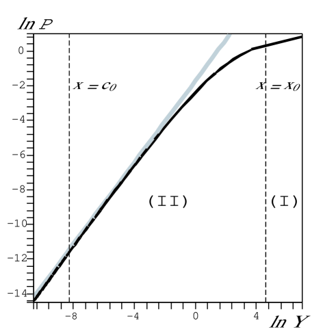
Figure 1: The thick curve is the plot of $\ln\,{\cal{P}}$ vs $\ln\,Y$, equivalent to plotting $\ln\,P$ vs $\ln\,\rho\,V_{0}^{2}$. The radius $x=x_{0}\approx 0.01\,c_{0}$, corresponding to the minimal resolution of numerical simulations, marks the “inner” region (I). The “outer” region (II) denotes the halo up to its physical radius, the virial radius $x=c_{0}=15$. As a comparison we show a line with slope $1.18$ (thick grey line) that would correspond to the poytropic relation with $n\approx 5.5$. Notice how the NFW halo approximately fits this relation, except near the center where the density profile becomes cuspy.

VII Discussion and conclussion

The fact that NFW halos asymptoticaly comply with a polytropic relation with $n\approx 5.5$ is quite significant, since stellar polytropes characterized by (45) are the equilibrium state associated with the entropy functional in the non–extensive entropy formalism derived by Tsallis and coworkers PL ; Tsallis ; TS1 ; TS2 . In its application to self–gravitating collisionless systems this formalism is characterized by the free parameter $q=(2n-1)/(2n-3)$, so that the isothermal sphere (equilibrium state for the usual Boltzmann–Gibbs entropy functional) follows in the “extensive entropy” limit $n\to\infty$ (or $q\to 1$). Assuming Tsallis theory to be correct, the empiric verification (see Figure 1) that NFW halos outside the “inner” core satisfy a polytropic relation might indicate that in this “outer” region the NFW numerical simulations yield self–gravitating configurations that approach an equilibrium state characterized by the Tsallis parameter $q\approx 1.25$. However, while the central cusps in the density profile that are predicted by NFW simulations seem to be at odds with observations cdm_problems_1 ; cdm_problems_2 , there is no conflict between these observations and the $1/x^{3}$ scaling of the NFW density profile outside the core region (as well as the rotation velocity profile from (40)). Although the issue of the cuspy cores is still controversial, if galactic halos seem to exhibit flat density cores, their profiles could be adjusted to stellar polytropes and this might be helpful in providing a better empirical verification of Tsallis’ formalism. However, this idea must be handled with due case, since stellar polytropes follow from an isotropic velocity distribution, while galactic halos with such distributions could be unrealistic.

As pointed out before, the density profile of NFW halos diverges at the center. Apparently this issue has not bothered astrophysicists, since (as mentioned before) the cuspy cores of NFW numerical simulations are meant to show a density scaling of $1/x$ near the center and these simulations cannot resolve distances to the halo center smaller than 1 % of the virial radius NSres . One way to deal with this unphysical feature, leading to a better description of these halos, would be to perform a smooth matching between NFW spacetimes and a small central region with a regular density profile. An adequate radius for this “inner” region could be the minimal resolution scale in numerical simulations ($x=x_{0}\sim 0.01\,c_{0}$). Another improvement could be a smooth matching of the NFW spacetime to a Schwarzschild vacuum exterior at the virial radius $x=c_{0}$, which is the physical radius of the halo. One of the matching conditions in this latter case would be ${\cal{P}}(c_{0})=0$, implying a different choice of the integration constant $C$ in (43). Another necessary improvement is the study of the anisotropic cases for which $\alpha\neq 0$.

We have constructed the spacetime corresponding to post–Newtonian generalizations suitable to NFW halos. Although we have presented only the idealized case with isotropic pressure, the methodology that we followed here can be applied, in principle, to any Newtonian model of galactic halos. We believe that it is necessary to study galactic halo models (NFW, as well as other empiric or theoretical models) within a wider framework including the usual thermodynamics of self–gravitation systems Padma2 ; Padma3 , as well as alternative approaches such as Tsallis’ formalism Tsallis ; PL ; TS1 ; TS2 . Such an improvement and extension of the present study of NFW halos are being pursued elsewhere enproceso .

VIII acknowledgements

It is a pleasure to participate with this work in the number dedicated to honor our friend and college Prof. Alberto García. RAS acknowledges financial support from grant PAPIIT-DGAPA number IN117803, DN does so from grant DGAPA-UNAM IN122002. TM acknowledges partial financial support by CONACyT México, under grants 32138-E and 34407-E.

References

- (1) E.W. Kolb and M.S. Turner: The Early Universe, Addison–Wesley Publishing Co., 1990.
- (2) T. Padmanabhan: Structure formation in the universe, Cambridge University Press, 1993.
- (3) J.A. Peacocok: Cosmological Physics, Cambridge University Press, 1999.
- (4) John Ellis, Summary of DARK 2002: 4th International Heidelberg Conference on Dark Matter in Astro and Particle Physics, Cape Town, South Africa, 4-9 Feb. 2002. e-Print Archive: astro-ph/0204059.
- (5) N. Fornengo, Proceedings of 5th International UCLA Symposium on Sources and Detection of Dark Matter and Dark Energy in the Universe (DM 2002), Marina del Rey, California, 20-22 Feb 2002. e-Print Archive: hep-ph/0206092.
- (6) D.N. Spergel and P.J. Steinhardt, Phys Rev Lett., 84, 3760, (2000); A. Burkert, APJ Lett., 534, 143, (2000); C. Firmani et al, MNRAS, 315, 29, (2000).
- (7) S. Colombi, S. Dodelson and L. Widrow, ApJ, 458, 1, (1996); R. Schaeffer and J. Silk, ApJ, 332, 1, (1998); C.J. Hogan, astro-ph/9912549; S. Hannestad and R. Scherrer, Phys. Rev. D, 62, 043522, (2000).
- (8) Tonatiuh Matos and F. Siddhartha Guzmán. Class. Quant. Grav., 17, (2000), L9-L16. See also: Tonatiuh Matos and Luis A. Ureña. Phys Rev. D63, (2001), 063506.
- (9) Tonatiuh Matos, F. Siddhartha Guzmán and Darío Núñez. Phys Rev. D62, (2000), 061301(R); Tonatiuh Matos, Darío Núñez, F. Siddhartha Guzmán and Erandy Ramirez. Gen. Rel. Grav., 34, (2002), in press. Available at: astro-ph/0005528. Tonatiuh Matos and F. Siddhartha Guzmán. Class. Quant. Grav., 18, (2001), 5055-5064.
- (10) U. Nucamendi, M. Salgado and D. Sudarsky, Phys. Rev. Lett., 84, 3037, (2000).
- (11) Luis G. Cabral–Rosetti et al, Class. Quant. Grav., 19, (2002), 3603–3615.
- (12) K. Lake, e-Print Archive: gr-qc/0302067.
- (13) E. Battaner and E. Florido, The rotation curve of spiral galaxies and its cosmological implications. astro-ph/0010475.
- (14) J. Binney and S. Tremaine: Galactic Dynamics, Princeton University Press, 1987.
- (15) J.F. Navarro, C.S. Frenk and S.D.M. White, ApJ, 462, 563, (1996); see also: J.F. Navarro, C.S. Frenk and S.D.M. White, ApJ, 490, 493, (1997).
- (16) B. Moore et al, MNRAS, 310, 1147, (1999).
- (17) S. Ghigna et al, astro-ph/9910166.
- (18) E Lokas and G Mamon, MNRAS, 321, 155, (2001)
- (19) B. Moore, Nature, 370, 629, (1994).
- (20) R. Flores and J. P. Primack, ApJ, 427, L1, (1994).
- (21) S.R. de Groot, W.A. van Leeuwen and Ch.G. van Weert, Relativistic Kinetic Theory. Principles and Applications, North Holland Publishing Company, 1980. See pp 46-55.
- (22) T. Padmanabhan: Phys. Rep. 188, 285 - 362 (1990).
- (23) T. Padmanabhan: Theoretical Astrophysics, Volume I: Astrophysical Processes, Cambridge University Press, 2000.
- (24) Tonatiuh Matos, Darío Núñez and Roberto A. Sussman, in preparation.
- (25) L.P. Ostipkov, PAZh, 5, 77, (1979); D. Merritt, AJ, 90, 1027, (1985)
- (26) E.L. Lokas and Y. Hoffman, astro-ph/0108283. See also E.L. Lokas Acta Phys.Polon., B32, 3643-3654, (2001)
- (27) V. R. Eke, J. F. Navarro, and M. Steinmetz, ApJ, 554, 114–120, (2001). See also J. Zavala, V. Avila–Reese, H. Hernandez–Toledo, and C. Firmani, A & A, 412, 633-650, (2003).
- (28) S. Ghigna et al, Ap J, 544, 616–628, (2000).
- (29) T. Matos and D. Núñez. The general relativistic geometry of the Navarro-Frenk-White model. e-Print Archive: astro-ph/0303594.
- (30) C, Tsallis, Braz J Phys, 29, 1; S. Abe and Y. Okamoto (Eds.), Nonextensive Statistical Mechanics and its Applications (Springer, Berlin, 2001
- (31) A. R. Plastino and A Plastino, Phys Lett A, 174, 384, (1993)
- (32) A. Taruya and M. Sakagami, Physica A, 307, 185–206, (2002); See also Physica A, 322, 285–312, (2003) and cond-mat/0204315.
- (33) A. Taruya and M. Sakagami, Phys Rev Lett, 90, 181101, (2003); See also cond-mat/0310082.