Period-color and amplitude-color relations in classical Cepheid variables

Abstract

In this paper we analyze the behavior of Galactic, LMC and SMC Cepheids in terms of period-color (PC) and amplitude-color (AC) diagrams at the phases of maximum, mean and minimum light. We find very different behavior between Galactic and Magellanic Cloud Cepheids. Motivated by the recent report of a break in LMC PC relations at 10 days (Tammann et al. 2002), we use the F-statistical test to examine the PC relations at mean light in these three galaxies. The results of the F-test support the existence of the a break in the LMC PC(mean) relation, but not in the Galactic or SMC PC(mean) relations. Furthermore, the LMC Cepheids also show a break at minimum light, which is not seen in the Galactic and SMC Cepheids. We further discuss the effect on the period-luminosity relations in the LMC due to the break in the PC(mean) relation.

1 Introduction

Simon, Kanbur & Mihalas (1993, hereafter SKM) used hydro-dynamical models to explain the observations of Code (1947): Galactic Cepheids show a spectral type independent of period at maximum light and a spectral type at minimum light that gets later as the period increases. SKM computed radiative hydro-dynamical models of Galactic Cepheids which agreed with Code’s observations. SKM interpreted these observational phenomena as being due to the location of the photosphere relative to the hydrogen ionization front. They further used the Stefan-Boltzmann law applied at maximum and minimum light to show that

$$\log T_{max}-\log T_{min}={1\over{10}}(V_{min}-V_{max}),$$ (1)

where $T_{max}$ and $T_{min}$ refer to the effective temperature at maximum and minimum light, respectively. Thus, higher optical amplitudes are associated with higher temperature amplitudes, which are in turn related to higher values of $T_{max}$ and/or $T_{min}$. For this study we do not assert a causal relation between higher temperatures and higher amplitudes preferring to refer to these quantities as being “associated”. If, for some reason, either $T_{max}$ or $T_{min}$ does not increase as the amplitude increases, equation (1) predicts a relationship between amplitude and $T_{min}$ or $T_{max}$ respectively. SKM used data from Pel (1976) and Moffett & Barnes (1980, 1984) to show that Galactic Cepheids are such that higher amplitude stars are driven to cooler temperatures at minimum light. This, according to equation (1), is because the range of temperatures at maximum light is independent of period for a large range of periods. So the form of the period-color (PC) relation at maximum light is related to the form of the amplitude-color (AC) relation at minimum light, and vice versa.

Tammann et al. (2003) used Galactic and OGLE LMC/SMC Cepheid data to show that there is a difference in the PC relations in these three galaxies. Furthermore, Tammann et al. (2002) and Tammann & Reindl (2002) show the existence of two PC relations, one for short ($P<10$ days) and one for long ($P>10$ days) period Cepheids, in the LMC. Motivated by this and the presence of high quality Magellanic Cloud Cepheid data from the OGLE project (Udalski et al., 1999a), we decided to investigate the properties of Magellanic Cloud Cepheids in terms of their PC and AC relations at maximum, mean and minimum light.

In addition to the two major reasons mentioned above, we list a number of other arguments motivating the present study:

1. Since mean light is just that - the average over a range of values - interesting properties of Cepheids at mean light are due to the average of these properties at all pulsation phases. By investigating the phases of maximum and minimum light, we are studying those phases of stellar pulsation which contribute to the observed properties at mean light. Our interest lies in understanding breaks in the LMC mean light Cepheid PC and period-luminosity (PL) relations at 10 days reported by Tammann et al. (2002). Let $y_{ij}$ be the (absolute) magnitude of Cepheid variable stars, $i=1,...,n_{star}$ at the $j^{th}$ phase ($j=1,...,N$) during a pulsation period $P_{i}$. Then we can formulate a PL relation at a particular phase as,

   $$y_{ij}=a_{j}+b_{j}\log(P_{i}),$$ (2)

   where $a_{j},b_{j}$ are the unknown coefficients as a function of the phase $j$. If we define $y_{i}$ as ${\sum_{j=1}^{j=N}y_{ij}}/N$, the average over the pulsation period, it is easy to show that $y_{i}=a_{m}+b_{m}\log(P_{i}),$ where $a_{m},b_{m}$ are the average over phase of the $a_{j},b_{j}$ in equation (2). This will be true if $y$ is measured in intensities and then the intensity mean converted to magnitudes or if $y$ is measured in magnitudes. Of course the magnitude mean and intensity means are in general not equal to each other but the difference is small ($\sim 0.03mag.$) and constant over a wide range of periods (for example, see Gieren et al. 1998). Consequently, some insight into the mean light relation can be gained by studying PL relations at various phases, e.g. at maximum and minimum light. Since the PC relation affects the PL relation (see, e.g., Madore & Freedman 1991 for the basic physics of PC and PL relations), it is of interest to study the PC relation at various phases. Furthermore, the maximum and minimum light are closely associated with the more interesting phases of stellar pulsation: the expansion/contraction velocity is close to its maximum value when the photosphere is passing through the mean radius of the star (see, e.g., Mihalas 2003 for the details).

2. The amplitude is a fundamental observational and theoretical quantity in stellar pulsation. Kanbur and Ngeow (2004, in-preparation) show that the amplitude is a very good descriptor of light curve shape, and the V band amplitudes are correlated to the first Principal Component ($PC1$) of the light curve. In addition, Kanbur et al. (2002) demonstrated that $PC1$ can explain over 90$\%$ of the variation in light curve shape. Thus the V band amplitude can be taken to be a good descriptor of V band light curve shape. A similar conclusion holds for the I band. Because the optical brightness fluctuations of Cepheids are predominantly due to temperature fluctuations (Cox, 1980), it is thus instructive to examine AC diagrams at maximum and minimum V band light. Furthermore, since AC relations are related to PC relations through equation (1), their study can serve as a useful complement to strengthen any conclusions reached using PC relations.

2 The Data

The standard Johnson-Cousins V and I band data for the fundamental mode Cepheids in the Galaxy, LMC and SMC were used in this study. For both of the LMC and SMC Cepheids, the periods, V and I band photometric data and the $E(B-V)$ values for every Cepheid were taken from the OGLE (Udalski et al., 1999b, c) website. There are 771 and 488 fundamental mode Cepheids (as classified by OGLE team) in LMC and SMC, respectively. For Galactic Cepheid data, we considered only the Cepheids classified as “DCEP” in the General Catalog of Variable Stars (GCVS, fourth edition, Kholopov 1998). The periods for the Galactic Cepheids are taken from the McMaster Cepheid database, and the $E(B-V)$ values are adopted from Tammann et al. (2003, listed as $E(B-V)_{corr}$ in their table 1). The photometric data for Galactic Cepheids were obtained from two sources: (a) Moffett & Barnes (1984), where actual data were downloaded from the McMaster Cepheid database; and (b) Berdnikov (1997) and Berdnikov & Turner (2001). For Cepheids that have entries in both Berdnikov (1997) and Berdnikov & Turner (2001), photometric data from these two sources were merged together to provide a better light curve. Since the bandpasses used in Moffett & Barnes (1984) are in Johnson V and I, we converted the Johnson I band photometric data in this dataset to Cousins I band with the color transformations given in Coulson et al. (1985).

The Cepheid photometric data in these three galaxies were then fitted with a Fourier expansion of the following form (Schaltenbrand & Tammann, 1971; Ngeow et al., 2003):

$$m(t) = m_{0}+\sum^{M}_{i=1}[A_{i}\cos(2\pi i\Phi(t)+\phi_{i})],$$ (3)

where $\Phi(t)=(t-t_{0})/P-int[(t-t_{0})/P]$, with $t_{0}$ being a common starting epoch for all Cepheids in both bands. We used a simulated annealing technique to fit the data with this Fourier expansion, as described in Ngeow et al. (2003). Thus our Fourier fits are carried out to published photometric data and our means are magnitude means. For Galactic data, we adopted a fifth order expansion ($M=5$) to most of the Cepheids. However, in certain cases a fourth or sixth order Fourier expansion gave a better fit to the data. For OGLE LMC Cepheids, we fit the data with $M=4$, as this dataset is also used in Ngeow et al. (2003) and in Kanbur et al. (2003). For OGLE SMC Cepheids, we mainly fit fourth or fifth order Fourier expansions to the data, while some of them were fitted with sixth order. All fitted light curves were then visually inspected (see Kanbur et al. 2003 for the selection criteria). Figure 7 of Ngeow et al. (2003) illustrates the improvement that can be obtained when using our fitting method to the observed light curves. We only selected those Cepheids with well fitted light curves in both V and I bands. In addition, we exclude Cepheids with $\log(P)<0.4$ to avoid possible contamination from first overtone Cepheids (Udalski et al., 1999a). The numbers of Cepheids in the final samples are: 79 from Moffett & Barnes (1984) data; 75 from Berdnikov data; 634 from OGLE LMC data; and 391 from OGLE SMC data. From the Fourier fits we obtained the following quantities:

1. V and I band amplitude from the numerical maximum and minimum of the Fourier fits: $V_{amp}=V_{min}-V_{max}$, $I_{amp}=I_{min}-I_{max}$.

2. $(V-I)_{max}$: defined as $V_{max}-I_{phmax}$, where $I_{phmax}$ is the I band magnitude at the same phase as $V_{max}$.

3. $(V-I)_{mean}$: defined as $V_{mean}-I_{phmean}$, where $I_{phmean}$ is the I band magnitude at the same phase as $V_{mean}$. $V_{mean}$ is the V band magnitude closest to $m_{0}$, the mean value in equation (3).

4. $(V-I)_{min}$: defined as $V_{min}-I_{phmin}$, where $I_{phmin}$ is the I band magnitude at the same phase as $V_{min}$.

Finally, the colors at these three phases have been corrected for extinction using $A_{V,I}=R_{V,I}E(B-V)$. The values of $R$ are: $R_{V}=3.17$, $R_{I}=1.89$ for Galactic data (Tammann et al., 2003), and $R_{V}=3.24$, $R_{I}=1.96$ for OGLE LMC and SMC data Udalski et al. (1999b, c). In fact, the results are unchanged for the values of $R_{V}$ and $R_{I}$ as long as $\Delta R\equiv R_{V}-R_{I}=1.28$ as given in Tammann et al. (2003), because $(V-I)_{o}=(V-I)-\Delta R\ E(B-V)$. We apply the same extinction values of $A_{V,I}$ to the colors at maximum, mean and minimum light, since the quantities of $A_{V,I}$ should remain unchanged for any pulsation phases. In addition, our results are unchanged if we adopt $(<V>-<I>)_{o}$ for the mean color as in item (iii) above.

  

Figure 1: The period-color and amplitude-color relations at phases of maximum, mean and minimum light for Galactic Cepheids. The open circles and filled circles correspond to short and long period Cepheids, respectively. The dashed and solid lines are the fitted period-color and amplitude-color relations to short and long period Cepheids, respectively. The number of short and long period Cepheids are $n_{short}=113$ and $n_{long}=41$. Left (a): The period-color relations. Right (b): The amplitude-color relations.

  

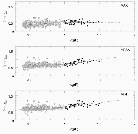
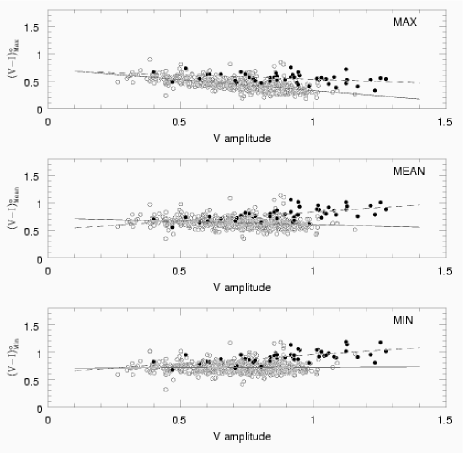
Figure 2: The period-color and amplitude-color relations at phases of maximum, mean and minimum light for OGLE LMC Cepheids. The open circles and filled circles correspond to short and long period Cepheids, respectively. The dashed and solid lines are the fitted period-color and amplitude-color relations to short and long period Cepheids, respectively. The number of short and long period Cepheids are $n_{short}=585$ and $n_{long}=49$. Left (a): The period-color relations. Right (b): The amplitude-color relations.

  

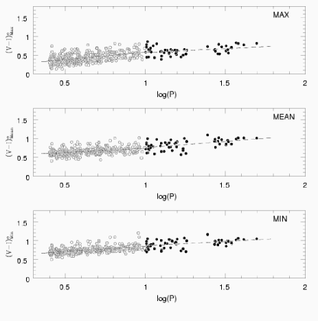
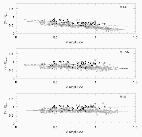
Figure 3: The period-color and amplitude-color relations at phases of maximum, mean and minimum light for OGLE SMC Cepheids. The open circles and filled circles correspond to short and long period Cepheids, respectively. The dashed and solid lines are the fitted period-color and amplitude-color relations to short and long period Cepheids, respectively. The number of short and long period Cepheids are $n_{short}=334$ and $n_{long}=57$. Left (a): The period-color relations. Right (b): The amplitude-color relations.

3 Analysis and Results

Figures 1, 2 and 3 show the plots of $\log(P)$ vs. $(V-I)_{o}$ color and $V_{amp}$ vs. $(V-I)_{o}$ color at maximum, mean and minimum light (see the definition in Section 2) for the Cepheids in Galaxy, LMC and SMC respectively. Open and closed circles in these figures are for short ($\log(P)<1.0$) and long ($\log(P)>1.0$) period Cepheids, respectively. In what follows short and long period Cepheids are always used in this sense. For all three data sets in the Galaxy, LMC and SMC, we can fit linear relations between $\log(P)$ and $(V-I)_{o}$ color and $V_{amp}$ and $(V-I)_{o}$ color, both for the entire sample, and also for short and long period Cepheids separately. Tables 1 and 2 show these results for the fits to period-color and amplitude-color relations, respectively. In these tables, column 1 gives the phase at which the fit is made - either at maximum, mean or minimum light. Column 2 is labelled $MRSS$ and represents the mean residual sum of squares from the fit to the entire sample. The slope of the linear fit together with its associated error is given in column 3. Columns 4 and 5 give the residual mean sum of squares and slope plus error for the short period Cepheids. Columns 6 and 7 do this for the longer period Cepheids. We discuss columns 8-11 shortly. In Figures 1-3 we have plotted the fitted lines for short and long period Cepheids as solid and dashed lines respectively.

What is of interest for the present study is whether these PC plots show statistical evidence of a change of slope at a period of 10 days. To investigate this, we can fit a regression line over the entire period range and then fit two regression lines, one separately for short and long period Cepheids. The former case is the reduced model while the latter case with two separate regression lines is the full model. We can write the model under consideration as

$$Y=a_{S}W_{S}+a_{L}W_{L}+b_{S}Z_{S}+b_{L}Z_{L}+\epsilon.$$ (4)

Here $Y$ is the dependent variable, in our case $(V-I)_{o}$ color at any of the three phases under consideration. $W_{S}$ is an indicator variable which is 1 if the star’s period is less than 10 days and 0 otherwise. $W_{L}$ is an indicator variable which is 0 if the star’s period is less than 10 days and 1 otherwise. The variable $Z_{S}$ contains the independent variable, either $\log(P)$ or $V_{amp}$, but is zero if the period is greater than 10 days. $Z_{L}$ is similar but is zero for periods less than 10 days. The parameters $a_{S}$, $a_{L}$, $b_{S}$ and $b_{L}$ are the zero-points and slopes for short and long period Cepheids, respectively. Thus what is of interest is if the data are consistent with $b_{L}=b_{S}$: the slope is same for long and short period Cepheids. Weisberg (1980) shows that in this situation an appropriate F test statistic can be formulated as described in the following equation,

$$F=\frac{(RSS_{R}-RSS_{F})/[(n-2)-(n-4)]}{RSS_{F}/(n-4)},$$ (5)

where $RSS_{R},RSS_{F}$ are the residual sums of squares in the reduced (single line regression) and full model (two lines regression), respectively, and $n$ is the number of stars in the entire sample. We refer the F statistic in equation (5) to an F distribution, $F_{2,n-4}$, under the null hypothesis that the two-parameter regression (i.e. a single line) is sufficient. The four-parameter regression (i.e. two lines) will have a smaller residual sum of squares. The probability of the observed value of the F statistic, $P(F)$, under the null hypothesis, gives the significance of this reduction in sum of squares. Thus, a “large” value of F indicates that the null hypothesis can be rejected. Column 8 of Tables 1 and 2 gives the values of the F statistic and column 9 gives its probability value as described above. Note that because there are fewer observed long period Cepheids, the error on the slope for the long period PC relations is generally larger but this is automatically taken account of by the F test.

It could also be that the short and long period slopes are similar but that the F statistic produces a significant result because the intercepts are different. In this case, we can also compare the statistical significance of differences in the slopes of these regressions by referring the quantity,

$$t = (b_{S}-b_{L})\frac{1}{S_{b_{S}-b_{L}}},$$ (6)

$$S_{b_{S}-b_{L}} = \sqrt{\frac{MS}{SS_{S}}+\frac{MS}{SS_{L}}},$$ (7)

$$MS = \frac{SS_{S}+SS_{L}}{n_{S}+n_{L}-4}$$ (8)

to a $t$ distribution with $n_{S}+n_{L}-4$ degrees of freedom. $P(t)$ is the probability of the observed value of the $t$ statistic under the null hypothesis that the two slopes are equal. In the above formulae $SS_{S},SS_{L},n_{S},n_{L},b_{S},b_{L}$ are the residual sum of squares, the number of Cepheids and the slopes in the PC or AC relation for short and long period Cepheids, respectively. Columns 10 and 11 in Tables 1 and 2 give the values of $t$ statistic and its associated $P(t)$ value from two-tail $t$ distribution.

Table 1: Period-color relations at maximum, mean and minimum light.

Phase	$MRSS_{all}^{a}$	$Slope_{all}^{b}$	$MRSS_{S}^{a}$	$Slope_{S}^{b}$	$MRSS_{L}^{a}$	$Slope_{L}^{b}$	F	P(F)	t	P(t)
(1)	(2)	(3)	(4)	(5)	(6)	(7)	(8)	(9)	(10)	(11)
					Galactic
Max	0.009	$0.142\pm 0.031$	0.006	$0.389\pm 0.062$	0.013	$0.020\pm 0.105$	7.95	0.00	3.40	0.00
Mean	0.008	$0.264\pm 0.030$	0.006	$0.229\pm 0.062$	0.013	$0.373\pm 0.104$	1.05	0.35	1.34	0.18
Min	0.007	$0.310\pm 0.028$	0.005	$0.330\pm 0.058$	0.013	$0.309\pm 0.104$	0.06	0.94	0.21	0.83
					OGLE LMC
Max	0.010	$0.205\pm 0.020$	0.010	$0.234\pm 0.030$	0.008	$-0.031\pm 0.101$	2.67	0.07	2.24	0.03
Mean	0.009	$0.239\pm 0.018$	0.008	$0.152\pm 0.027$	0.007	$0.590\pm 0.097$	13.19	0.00	4.10	0.00
Min	0.008	$0.291\pm 0.018$	0.008	$0.204\pm 0.027$	0.009	$0.493\pm 0.109$	10.38	0.00	2.73	0.01
					OGLE SMC
Max	0.013	$0.324\pm 0.021$	0.013	$0.396\pm 0.039$	0.011	$0.207\pm 0.071$	3.16	0.04	2.23	0.03
Mean	0.008	$0.272\pm 0.017$	0.007	$0.229\pm 0.030$	0.012	$0.340\pm 0.074$	1.77	0.17	1.65	0.10
Min	0.007	$0.276\pm 0.015$	0.006	$0.282\pm 0.027$	0.010	$0.229\pm 0.066$	0.42	0.66	0.87	0.38

• ^a $MRSS$ denotes mean of residual sum of squares from the fit. $MRSS_{all}$, $MRSS_{S}$ and $MRSS_{L}$ are for the fits to all, short and long Cepheids in the sample, respectively.

• ^b Slopes for the period-color relations for all, short and long period Cepheids in the sample.

Table 2: Amplitude-color relations at maximum, mean and minimum light.

Phase	$MRSS_{all}^{a}$	$Slope_{all}^{b}$	$MRSS_{S}^{a}$	$Slope_{S}^{b}$	$MRSS_{L}^{a}$	$Slope_{L}^{b}$	F	P(F)	t	P(t)
(1)	(2)	(3)	(4)	(5)	(6)	(7)	(8)	(9)	(10)	(11)
					Galactic
Max	0.010	$-0.098\pm 0.042$	0.007	$-0.313\pm 0.058$	0.012	$-0.169\pm 0.088$	15.54	0.00	1.50	0.14
Mean	0.010	$0.241\pm 0.042$	0.007	$0.011\pm 0.059$	0.014	$0.275\pm 0.095$	10.98	0.00	2.65	0.01
Min	0.009	$0.322\pm 0.041$	0.007	$0.145\pm 0.058$	0.013	$0.276\pm 0.089$	9.76	0.00	1.36	0.18
					OGLE LMC
Max	0.010	$-0.285\pm 0.023$	0.007	$-0.393\pm 0.023$	0.007	$-0.160\pm 0.058$	93.12	0.00	3.62	0.00
Mean	0.011	$0.016\pm 0.025$	0.008	$-0.118\pm 0.024$	0.008	$0.322\pm 0.064$	95.99	0.00	6.42	0.00
Min	0.011	$0.140\pm 0.025$	0.009	$0.017\pm 0.025$	0.009	$0.321\pm 0.065$	92.66	0.00	4.33	0.00
					OGLE SMC
Max	0.010	$-0.438\pm 0.021$	0.007	$-0.419\pm 0.018$	0.010	$-0.308\pm 0.070$	80.45	0.00	1.79	0.07
Mean	0.012	$-0.158\pm 0.023$	0.007	$-0.144\pm 0.019$	0.017	$0.034\pm 0.092$	75.40	0.00	2.54	0.01
Min	0.012	$-0.065\pm 0.023$	0.008	$-0.047\pm 0.020$	0.011	$0.104\pm 0.076$	82.45	0.00	2.21	0.03

• ^a $MRSS$ denotes mean of residual sum of squares from the fit. $MRSS_{all}$, $MRSS_{S}$ and $MRSS_{L}$ are for the fits to all, short and long Cepheids in the sample, respectively.

• ^b Slopes for the amplitude-color relations for all, short and long period Cepheids in the sample.

Our figures do not contain error bars on the estimated values of the $(V-I)_{o}$ color. These error bars are typically less than the size of the symbol. This includes errors due to photometry and reddening. A typical V band photometric error quoted by the OGLE team is $0.015mags$ and perhaps as much as $0.05mags$ for reddening. If we add these in quadrature, a rough estimate of sigma for the photometry is $0.052mags$. If we assume a similar figure for the I band (with errors of $\sim 0.001mags.$ to $0.005mags$) and again add up the errors in quadrature, then a typical error for the $(V-I)_{o}$ color is $\sim 0.07mags$. Strictly speaking this error should be included in a weighted least squares fit when constructing our period-color or amplitude-color fits. The weights are the inverse of the error assigned to each data point. However if the weights are constant for each star then they cancel out in the calculation of the F statistic and in the derivation of the coefficients of the linear regression. Hence the only way that inclusion of errors in our least squares fits can affect the significance of our F statistic results is if the errors are systematically greater for large numbers of either short or long period Cepheids. If this is the case, it will affect not only our work but also published values of the LMC PL relations in the V and I band (e.g., in Udalski et al. 1999a).

We now discuss the assumptions required by the F test. These are that the error ($\epsilon$) in equation (4) is constant for all the stars in our study, and further they are normally distributed with zero mean. To test these assumptions, we analyze the OGLE LMC data in greater detail. Figure 4 shows the plots of residuals from a single PC fit and two PC fits to the entire data against $\log(P)$. We see no discernible trend in the size of the residuals with period and are led to the conclusion that the residuals are homoskedastic (i.e. $\sigma\sim$ constant). This supports our approach of adopting a constant $\sigma$ to gauge photometric errors when doing a least squares fit. In addition, the residuals in Figure 4 from the fit with a single PC relation show a trend (though not in the size of the residuals) in long period Cepheids, which is reduced when using two PC relations for short and long period Cepheids to fit the data. In order to test that the residuals are normally distributed, we can plot the quantiles of the distribution resulting from the ordered residuals against the expected quantiles from a normal distribution: a qq-plot. If the residuals are indeed normally distributed then this plot should be close to the line $y=x$. Figure 5 shows such a plot. There is some small departure from normality at the extremes but we contend that this plot justifies our use of the F test.

 

Figure 4: Plots of the residuals of LMC period-color relation at mean light. Top: (a) The residuals from the long and short period PC relations as a function of $\log(P)$. Bottom: (b) The residuals from using a single PC relation as function of $\log(P)$. From the plots it is clear that the residuals are homoskedastic. In addition, the residuals from the fit with a single PC relation show a trend in long period Cepheids. This trend is reduced if two PC relations were used to fit the data.

 

Figure 5: Plot of the ordered residual quantiles vs. normal quantiles, the qq-plot. The line is the case of $y=x$.

There is a great deal of information in Table 1 & 2, but for the context of the present study we summarize the results in the following subsections.

3.1 Results of period-color relations

For the Galactic Cepheids, the slope of the long period PC relation at maximum light is close to zero. Further, the overall slope at maximum light is the shallowest. This then supports the work of Code (1947). In addition, the F and $t$ test indicates that the PC relation at maximum light is not consistent with a single slope. However, the mean and minimum light PC relations for the Galactic Cepheids are consistent with a single line.

For the LMC Cepheids, the slopes of the long period PC relation at maximum light is also close to zero, decreasing significantly from its value for short period Cepheids. The slope at mean and minimum light all increase when going from short to long period Cepheids. In the LMC, we see that the PC relation at maximum light is not consistent with a single line at the 93$\%$ confidence level. However, in terms of the F test, the PC relation at mean and minimum light does show evidence to support a break at 10 days. Note that at both these phases, the slope of the PC relation for longer period Cepheids is much steeper than for shorter period Cepheids.

In the case of the SMC again the PC relation at maximum light is much flatter for longer period Cepheids than for shorter period. The relation at mean light for longer periods is steeper than at shorter period. Only the PC relation at maximum light shows statistical evidence of a break at 10 days.

We note that the slope of PC relation at maximum light always decreases in going from short to long period Cepheids in all three galaxies. In contrast, the slope at mean and minimum light always increases except for the Galactic and SMC Cepheids at minimum light. We also make the interesting observation that the dispersion of the PC relation, whether for the entire sample or either short or long period group, is always the smallest at minimum light in these three galaxies. A glance at the F statistic for mean light for the LMC Cepheids shows that we can reject the null hypothesis of a single PC relation for long and short period LMC Cepheids at greater than the 99$\%$ confidence level, confirming the finding of the broken PC relation in LMC (Tammann & Reindl, 2002; Tammann et al., 2002). However, the Galactic and SMC mean light PC relation is consistent with one line.

3.2 Results of amplitude-color relations

The AC relations all show statistical evidence of two lines at greater than $99.9\%$ confidence level with the F test. At mean and minimum light, we see that the slopes of the AC relation increase significantly when going from short to long period Cepheids in all three galaxies. However at maximum light the slope becomes shallower for long period Cepheids. Also, the slopes of the AC relation at maximum light are always negative for both short and long periods Cepheids in Galaxy, LMC and SMC, which we do not see in the mean and minimum light. In addition, the slopes are flat for the short period Galactic Cepheids and long period SMC Cepheids at mean light, but not for the Cepheids in LMC.

We also remark on some important differences in the AC plane between Galactic and Magellanic Cloud Cepheids. At minimum light in the LMC and SMC, the slope of the AC relation is $0.017\pm 0.025$ and $-0.047\pm 0.020$, respectively, for short period Cepheids, whereas it is $0.145\pm 0.058$ for Galactic Cepheids - more than $2\sigma$ difference. For longer period Cepheids in the LMC and SMC, this slope becomes positive ($0.321\pm 0.065$ and $0.104\pm 0.076$), whilst the longer period AC slope in the Galaxy is always significantly above zero.

Even though Table 2 shows that AC relations are significantly different for short and long period Cepheids in the SMC, Figure 3(b) suggests that the effect is much reduced in the SMC as compared to, e.g. Figure 1(b). One possible reason for this is that SMC Cepheids have lower amplitudes than LMC or Galactic Cepheids (Paczyński & Pindor, 2000). Equation (1) shows that even if the range of $T_{max}$ or $T_{min}$ is narrow, but if the amplitudes are not large, then $T_{min}$ or $T_{max}$ will not be driven to such low or high values.

3.3 Combining the PC and AC relations

As discussed in the Introduction, equation (1) predicts that if the PC relation is flat at maximum light, then there will be an AC relation at minimum light, and vice versa. We see some evidence to support this idea from Figure 1-3, and from Table 1 & 2. In summary:

Galactic short period Cepheids: PC relation steep at maximum $\rightarrow$ AC $\sim$flat at minimum.

Galactic long period Cepheids: PC relation flat at maximum $\rightarrow$ AC relations $\sim$steep at minimum. PC relation steep at minimum $\rightarrow$ AC relation $\sim$flat at maximum.

LMC short period Cepheids: PC relation $\sim$steep at maximum $\rightarrow$ AC relation flat at minimum.

LMC long period Cepheids: PC relation flat at maximum $\rightarrow$ AC relations steep at minimum; PC relation steep at minimum $\rightarrow$ AC relation $\sim$flat at maximum.

SMC short period Cepheids: PC relation steep at maximum $\rightarrow$ AC relation $\sim$flat at minimum.

4 Conclusion and Discussion

We have presented in Figures 1-3 new observational characteristics of Cepheids. Following the work of Tammann et al. (2002), we apply rigorous statistical tests to show that at mean light, there is a change in the LMC PC relation between short ($\log(P)<1.0$) and long period Cepheids, as shown in Figure 2(a). In addition, the LMC data also exhibit a change in the PC relation at minimum light. However, we find no such change at mean and minimum light in the Galactic and SMC Cepheids. We also find that the PC relations at minimum light generally show the smallest scatter among the three galaxies, as compare to the phases at maximum or mean light. Following the work of SKM we study amplitude-color diagrams at maximum, mean and minimum light and find very different behavior in the three galaxies for short and long period Cepheids. This difference not only occurs within a given galaxy between the short and long period Cepheids, but also occurs from galaxy to galaxy. For example, the behavior of short and long period Cepheids in the LMC is very different (i.e. Figure 2), and the behavior of Galactic and LMC Cepheids of short period is also very different. Thus we note that there is an effect with both period and metallicity. Further work with state of the art pulsation codes is under way to confront these observations with model calculations. In addition, the PC relations clearly show greater structure than a simple two line regression as used here. For example, the LMC data indicates another break at $\log(P)\sim 1.2$ (see, e.g., Figure 4). This will be the subject of a future paper.

4.1 Testing of Systematics

In this subsection we discuss some of the systematic effects that may affect our results, as follows:

1. Could reddening errors produce the results displayed in Figures 1-3? Consider the bottom panels of Figure 1(b) and 2(b) showing AC relations at minimum light for the Galaxy and LMC. In contrast to the Galactic counterpart, the AC relation for short period LMC Cepheids is flat. It is difficult to imagine a situation where the published reddening for these short period stars are in error to the extent of making this relation flat when it should have a slope like the Galactic relation. Furthermore, we use the $E(B-V)$ values from the literature, which would not only affect our results but also other published results that are based on these values.

2. Could outliers, perhaps stars that have been misclassified as Cepheids, produce our significant results? We examine the OGLE LMC Cepheid data to investigate this question. The plot of mean $(V-I)_{o}$ color against $\log(P)$ in the middle panel of Figure 2(a) shows a number of stars which seem to have very red colors. We exclude these stars and repeat our analysis for PC relations in the LMC. We note that it is possible to reduce the significance of our result at mean light by excluding stars that are too red. However if we exclude stars that are too blue, the F test again becomes significant. This conclusion can be seen in Table 3, where we apply various color cuts to the LMC data and then calculate the F test. Excluding the Cepheids with too red or blue color does not alter the results we have in Section 3.1.

3. Could we reduce the significance of our results by “judiciously” removing certain stars? Since we only consider stars with $\log(P)>0.4$, if we extend this cutoff to 0.6 ($P$ = 3.98 days) and repeat our analysis, we get very similar results. Also, excluding some of the longer period Cepheids, those with periods greater than $\log(P)>1.4$ increases the significance of our results. Hence the period cut we applied in this study would not significantly alter the results or conclusions we have.

Table 3: F test significance results with color cuts for LMC Cepheids.

$(V-I)_{o}$	$F$	$P(F)$	$F$	$P(F)$	$F$	$P(F)$
Range	Max	Max	Mean	Mean	Min	Min
0 - 1.9	2.67	0.07	13.2	0.00	10.4	0.00
0 - 1.1	2.95	0.05	14.0	0.00	10.7	0.00
0 - 1.0	4.45	0.01	10.4	0.00	7.86	0.00
0 - 0.9	3.34	0.04	7.69	0.00	6.38	0.00
0.3 - 1.9	2.67	0.07	13.2	0.00	10.4	0.00
0.4 - 1.9	2.48	0.08	14.8	0.00	12.2	0.00
0.5 - 1.9	2.41	0.09	16.3	0.00	13.0	0.00
0.5 - 0.9	3.16	0.04	10.4	0.00	8.76	0.00

While excluding stars based on color or period cuts as mentioned above, in some cases, can reduce the significance of our F test results at mean light (though never to a $P(F)$ value less than 0.1), such experiments have very little effect at minimum light. If we accept the assertion that mean light properties of Cepheids are an average of Cepheid properties at all pulsation phases, then irrespective of mean light, Tables 1-2 and Figures 1-3 clearly demonstrate a significant change in Cepheid observational properties between short and long period Cepheids in the Galaxy, LMC and SMC. Further if we accept these exclusions, they would also have an effect on the PL relations in both V and I bands and hence on the currently accepted extra-galactic distance scale.

4.2 The period-luminosity relations in LMC

Since the PL relation is affected by the PC relation, it is of interest to examine the PL relation in the OGLE LMC Cepheids, which show a break in the PC relation. Do the LMC data support a single PL relation or is the data consistent with a break at a period of 10 days as shown in Tammann et al. (2002)? We can use the F test to investigate the LMC PL relations in the V and I band as in Section 3. The results of the F test are shown in Table 4, where column 1 displays the phase and column 2 and 3 show the F statistic and its probability, under the null hypothesis of a single line, for the V band PL relations. Similar results for I band PL relations are listed in column 4 and 5 in Table 4. From the table, both V and I band PL relations at mean and minimum light are significant - that is the data are more consistent with a model where the slopes of the V and I band PL relation are different for short and long period Cepheids. However, the data are consistent with a single slope, in both V and I bands, for the PL relation at maximum light, even though the corresponding PC relation shows some evidence of a break at 10 days (see Table 1).

The actual slopes of the V and I band PL relation at maximum, mean and minimum light for short and long period Cepheids are given in Table 5. The second column in this table gives the overall slope. The third and fourth column give the short period and long period slopes, respectively. We clearly see that the slope at maximum light is virtually identical for short and long period Cepheids in both V and I bands. This is very different to the situation at mean and minimum light. How can the PC relation at maximum light show evidence of a break at $\log(P)=1.0$ yet the PL relation in V and I be consistent with one PL relation? This is certainly not the case for the PL relation at mean light in the LMC. This occurs because the LMC PC relation at mean light becomes steeper for long period Cepheids whereas at maximum light, the PC relation in the LMC becomes shallower for longer period Cepheids. Since the PC relation affects the PL relation, this shallow dependence at maximum light for longer period Cepheids suggests that the PL relation at that phase would not be affected too much. A detailed analysis of the PL relations at maximum, mean and minimum light will be presented in forthcoming paper.

Table 4: F test significance results for the LMC PL relation

phase	$F_{V\ band}$	$P(F)_{V\ band}$	$F_{I\ band}$	$P(F)_{I\ band}$
Max	0.32	0.73	0.04	0.96
Mean	8.86	0.00	6.25	0.00
Min	17.5	0.00	19.0	0.00

Table 5: Slopes of the V and I band PL relation at maximum, mean and minimum light for Cepheids in the LMC.

Phase	V slope (all)	V slope (short)	V slope (long)
Max	$-2.74\pm 0.05$	$-2.73\pm 0.08$	$-2.97\pm 0.26$
Mean	$-2.75\pm 0.04$	$-2.95\pm 0.07$	$-2.35\pm 0.25$
Min	$-2.59\pm 0.04$	$-2.85\pm 0.06$	$-1.84\pm 0.26$
Phase	I slope (all)	I slope (short)	I slope (long)
Max	$-2.95\pm 0.03$	$-2.96\pm 0.05$	$-2.94\pm 0.19$
Mean	$-2.99\pm 0.03$	$-3.10\pm 0.04$	$-2.94\pm 0.18$
Min	$-2.88\pm 0.03$	$-3.06\pm 0.04$	$-2.33\pm 0.17$

4.3 Future work

We new briefly summarize other implications from the present study. However, the detailed analysis of these topics are beyond the scope of this paper, and will be addressed in future papers.

1. Metallicity dependence on PC relation: From the period-mean density relation for a pulsator and the Stefan-Boltzmann law, it is easy to show that: $\log(P)=\alpha\log(L)+\beta\log(M)+\gamma\log(T_{eff})+const$. The parameters ($\alpha,\beta,\gamma$) and the constant term can be determined from stellar pulsation calculations. For example:

   $\log(P)=0.84\log(L)-0.68\log(M)-3.48\log(T_{eff})+const.$, from van Albada & Baker (1973).

   $\log(P)=0.93\log(L)-0.77\log(M)-3.54\log(T_{eff})+const.$, from Simon & Young (1997).

   $\log(P)=0.82\log(L)-0.60\log(M)-3.55\log(T_{eff})+const.$, from Beaulieu et al. (2001).

   In addition, the luminosity and mass should also obey an M-L relation from stellar evolution calculations. This M-L relation predicts that lower metallicity Cepheids will have higher luminosity (see, e.g., Bono et al. 2000) for given mass. Hence, at fixed period, lower metallicity Cepheids should be hotter than higher metallicity Cepheids. For example, Laney & Stobie (1986) showed that the long period SMC Cepheids are hotter than LMC Cepheids at given period by $\sim 200K$.

   Since the Magellanic Clouds (MC) have lower metallicity than the Galaxy, Cepheids in the MC should be bluer than Galactic Cepheids. Tammann et al. (2003) have reported this finding in their paper. In this study, we also found that the short period MC Cepheids generally have bluer $(V-I)_{o}$ color than Galactic Cepheids, for a given period, at maximum, mean and minimum light. However, larger errors in the PC relations for long period Cepheids make such a statement more contentious for long period Cepheids. We intend to investigate this in detail in a future paper.

2. Estimation of color excess: Fernie (1994) used the theory of SKM and the original suggestion of Code (1947) to establish a relation between $(B-V)$ color at maximum light, the $V$ band amplitude, period and the color excess $E(B-V)$ for Galactic Cepheids. Figure 1 shows that another approach would be using the properties of Cepheids at minimum light to estimate the color excess, since the PC relations at minimum light in generally show a smaller dispersion (see Section 3.1). Furthermore, the Galactic PC relation at maximum light indicates a break at 10 days (Table 1), but not in the PC relation at minimum light. In future work, we plan to investigate the possibility of using this relation as a way to determine reddening.

References

- Beaulieu et al. (2001) Beaulieu, J. P., Buchler, J. R. & Kolláth, Z., 2001, A&A, 373, 164
- Berdnikov (1997) Berdnikov, L. N., 1997, VizieR Online Data Catalog: CDS II/217
- Berdnikov & Turner (2001) Berdnikov, L. N. & Turner, D. G., 2001, ApJS, 137, 209
- Bono et al. (2000) Bono, G., Caputo, F., Cassisi, S., Marconi, M., Piersanti, L. & Tornambé, A., 2000, ApJ, 543, 955
- Code (1947) Code, A. D., 1947, ApJ, 106, 309
- Coulson et al. (1985) Coulson, I. M., Caldwell, J. A. & Gieren, W. P., 1985, ApJS, 57, 595
- Cox (1980) Cox, J. P., 1980, Theory of Stellar Pulsation, Princeton University Press, Ed.
- Fernie (1994) Fernie, J. D., 1994, ApJ, 429, 844
- Gieren et al. (1998) Gieren, W., Fouqué, P. & Gómez, M, 1998, ApJ, 496, 17
- Kanbur et al. (2002) Kanbur, S., Iono, D., Tanvir, N. R. & Hendry, M. A., 2002, MNRAS, 329, 126
- Kanbur et al. (2003) Kanbur, S., Ngeow, C., Nikolaev, S., Tanvir, N. & Hendry, M., 2003, A&A, 411, 361
- Kholopov (1998) Kholopov, P. N. et al., 1998, Combined General Catalogue of Variable Stars, 4.1 Ed. (CDS II/214A)
- Laney & Stobie (1986) Laney, C. D. & Stobie, R. S., 1986, MNRAS, 222, 449
- Madore & Freedman (1991) Madore, B. & Freedman, W., 1991, PASP, 103, 933
- Mihalas (2003) Mihalas, D., 2003, in Stellar Atmosphere Modeling, ASP Conf. Series Vol. 288, eds. Hubeny, Mihalas & Werner, pg 471
- Moffett & Barnes (1980) Moffett, T. J. & Barnes, T. G., 1980, ApJS, 44, 427
- Moffett & Barnes (1984) Moffett, T. J. & Barnes, T. G., 1984, ApJS, 55, 389
- Ngeow et al. (2003) Ngeow, C., Kanbur, S., Nikolaev, S., Tanvir, N. & Hendry, M., 2003, ApJ, 586, 959
- Paczyński & Pindor (2000) Paczyński, B. & Pindor, B., 2000, ApJL, 533, L105
- Pel (1976) Pel, J. W., 1976, Ph.D. thesis, University of Leiden
- Schaltenbrand & Tammann (1971) Schaltenbrand, R. & Tammann, G., 1971, A&AS, 4, 265