CMB constraints on interacting cosmological models

Abstract

Non–canonical scaling of the form $\rho_{x}\propto\rho_{m}a^{\xi}$, where $\rho_{x}$ and $\rho_{m}$ are the energy densities of dark energy and dark matter, respectively, provides a natural way to address the coincidence problem -why the two densities are comparable today. This non–canonical scaling is achieved by a suitable interaction between the two dark components. We study the observational constraints imposed on such models from the cosmic microwave background (CMB) anisotropy spectrum. Using the recent WMAP results for the location of the CMB peaks, we determine the admissible parameter space and find that interacting models are well consistent with current observational bounds.

I Introduction

The picture that emerges from the present cosmological observations portrays a spatially flat, low matter density universe, currently undergoing a stage of accelerated expansion cmbsuper . Within Einstein’s relativity, the simplest explanation for this acceleration requires two dark components: one in the form of non–luminous dust (“dark matter”) with negligible pressure, contributing roughly one-third of the total energy density of the Universe and clustering gravitationally at small scales, and the other one a smoothly distributed component having a large negative pressure (“dark energy”) and contributing about two–thirds of the total energy density of the Universe. Although the immediate candidate for this dark energy is the vacuum energy (i.e., a cosmological constant $\Lambda$), alternative scenarios, with acceleration driven by a dynamical scalar field, called “quintessence”, were proposed from different perspectives diff .

One problem that afflicts most of the models proposed so far is the so–called “coincidence problem” or “why now?” problem stein . The essence of this problem is as follows: as these two dark components redshift with expansion at different rates one may ask “why the ratio of these two components is of the same order precisely today?, i.e., why $\frac{\rho_{m}}{\rho_{x}}|_{0}={\cal O}(1)$ ?” There have been different approaches for solving it anek ; diego1 . The one to be discussed here considers some non–canonical scaling of the ratio of dark matter and dark energy with the Robertson–Walker scale factor $a(t)$ Dalal ; scaling

$$\frac{\rho_{m}}{\rho_{x}}\propto a^{-\xi}\ ,$$ (1)

where $\rho_{m}$ and $\rho_{x}$ are the energy densities of the dark matter and the dark energy, respectively, and the scaling parameter $\xi$ is a new quantity which assesses the severity of the problem. Thus, $\xi=3$ corresponds to the $\Lambda$CDM model and $\xi=0$ to the self similar solution with no coincidence problem. Hence, any solution with a scaling parameter $0<\xi<3$ makes the coincidence problem less severe. The standard noninteracting cosmology is characterized by the relation $\xi=-3w_{x}$, where $w_{x}\equiv p_{x}/\rho_{x}$ is the equation of state parameter for the dark energy which we here assume to be constant for simplicity. Solutions deviating from this relation represent a testable, nonstandard cosmology. Such deviation from standard dynamics can be obtained if the two dark components are not separately conserved but coupled to each other. This proposal has been explored in scaling ; plb and looks promising as a suitable mutual interaction can make both components redshift coherently.

Now, it seems advantageous to use the available observational information to constrain the nature of dark energy with minimal theoretical input rather than to perform a detailed fit to a particular model with a specific potential. This approach has been followed in Dalal , where high redshift supernovae survey, Alcock–Paczynski test to quasar pairs and evolution of cluster abundances have been used to constrain the scaling parameter $\xi$ and the dark energy equation of state parameter $w_{x}$ for the case of separately conserved components. As shown in scaling the high redshift SNIa data given in perl cannot discriminate between interacting models and the “concordance” $\Lambda$CDM model. Therefore, the target of this work is to constrain the parameters $\xi$ and $w_{x}$ for this kind of non–standard cosmology with the Cosmic Microwave Background (CMB) anisotropy spectrum. To this end, we use the Wilkinson Microwave Anisotropy Probe (WMAP) wmap and BOOMERanG boom data for the location of the peaks in the angular spectrum. As it turns out, the scaling interacting cosmology is well consistent with the observational bounds. The parameter space corresponding to interacting models, seems even to be favoured compared with the parameter space of the standard noninteracting models.

Section 2 succinctly recalls and slightly generalizes, by introducing a radiation component, the scaling model of Ref.scaling ; this component is crucial, of course, if one wishes to test the interacting cosmology with the CMB data. In section 3 the positions of the CMB peaks as witnessed by WMAP are used to constrain the model. Section 4 summarizes our findings. Finally, the Appendix collects the set of formulae employed in our analysis.

II Scaling Solutions

We consider a Friedmann–Lemaître–Robertson–Walker (FLRW) universe such that its total energy density consists of radiation (whose energy density lies at present by four orders of magnitude below that of matter), matter with negligible pressure (that encompasses both baryonic and non–baryonic components) and dark energy,

$$\rho=\rho_{r}+\rho_{m}+\rho_{x}\ .$$ (2)

The corresponding pressures are

$$p_{r}=\textstyle{1\over{3}}\rho_{r},\quad p_{m}<<\rho_{m},\quad p_{x}=w_{x}\rho_{x}\ .$$ (3)

The $m$ and $x$ components are supposed to share some coupling so that their energy densities obey the balances

$$\dot{\rho}_{r}+4H\rho_{r}=0\ ,$$ (4)

$$\dot{\rho}_{m}+3H\rho_{m}=Q\,,$$

$$\dot{\rho}_{x}+3H(1+w_{x})\rho_{x}=-Q\ ,$$ (5)

where $H\equiv\dot{a}/a$ is the Hubble factor and the (non-negative) quantity $Q$ measures the strength of the interaction. For simplicity this setup is chosen such that the entire matter component takes part in the coupling. Alternatively, one may treat the baryonic component as separately conserved. The constraints obtained below do not depend on whether or not the baryons are included in the interaction.

From Eq. (4) it follows that the radiation redshifts as

$$\rho_{r}=\rho_{r0}\left(\frac{a_{0}}{a}\right)^{4}\ ,$$ (6)

where $a_{0}$ is the current value of the scale factor.

We are interested in solutions with the following scaling behaviour for the two dark components,

$$\frac{\rho_{m}}{\rho_{x}}=r_{0}\left(\frac{a_{0}}{a}\right)^{\xi}\ ,$$ (7)

where $r_{0}$ denotes the ratio of both components at present time and $\xi$ is a constant parameter in the range $0\leq\xi\leq 3$. In scaling , it was shown that such scaling solutions follow from an interaction characterized by

$$Q=-3H\,\frac{(\xi/3)+w_{x}}{1+r_{0}(1+z)^{\xi}}\,\rho_{m}\ ,$$ (8)

where $1+z=a_{0}/a(t)$. For the standard cosmology without interaction - i.e., when $Q=0$ -, we have $\xi=-3w_{x}$. The $\Lambda$CDM model $(w_{x}=-1)$ is the special case with $\xi=3$. Any deviation from $Q=0$, i.e, $(\xi/3)+w_{x}=0$, implies an alternative, testable, non–standard cosmology. With the interaction (8) it is straightforward to find

$$\rho_{m}+\rho_{x}=\rho_{m0}\,\frac{1+r_{0}}{r_{0}}(1+z)^{3(1+w_{x})}\left[\frac{1+r_{0}(1+z)^{\xi}}{1+r_{0}}\right]^{-\frac{3w_{x}}{\xi}}\ .$$ (9)

Again, for $w_{x}=-1$ and $\xi=3$ this reduces to

$$\rho_{m}+\rho_{x}=\frac{\rho_{m0}}{r_{0}}[1+r_{0}(1+z)^{3}]\ ,$$ (10)

which is indeed the prediction of the $\Lambda$CDM model.
With the evolution of the components as given in Eqs.(6) and (9), the Friedmann equation can be written as

$$H^{2} = \frac{8\pi G}{3}\rho$$ (11)

$$= H_{0}^{2}\,\left[\Omega_{m0}\frac{1+r_{0}}{r_{0}}(1+z)^{3(1+w_{x})}\left[\frac{1+r_{0}(1+z)^{\xi}}{1+r_{0}}\right]^{-\frac{3w_{x}}{\xi}}\right.$$

$$+\left.\Omega_{ro}(1+z)^{4}\right]\ ,$$

where we have introduced the dimensionless density parameters

$$\Omega_{m0}=\frac{\rho_{m0}}{\rho_{c}}\ ,\quad\Omega_{x0}=\frac{\rho_{x0}}{\rho_{c}}\ ,\quad\Omega_{r0}=\frac{\rho_{m0}}{\rho_{c}}\ ,\quad\rho_{c}\equiv\frac{3H_{0}^{2}}{8\pi G}\ .$$ (12)

We can recast the last equation into

$$H^{2}=\Omega_{m0}H_{0}^{2}(1+z)^{4}\;X(z)\ ,$$ (13)

with

$$X(z)=\frac{1+r_{0}}{r_{0}}\,(1+z)^{3(1+w_{x})-4}\left[\frac{1+r_{0}(1+z)^{\xi}}{1+r_{0}}\right]^{-\frac{3w_{x}}{\xi}}+\frac{\Omega_{r0}}{\Omega_{m0}}\ .$$ (14)

The above form of $H^{2}$ is useful in testing various models against CMB observation card .

III Constraints from CMB

The CMB acoustic peaks and troughs arise from oscillations of the primeval plasma just before the Universe becomes translucent. These oscillations are the result of a balance between the gravitational interaction and the photon pressure in the tightly bound photon-baryon fluid. The locations of the peaks corresponding to different angular momenta depend on the acoustic scale $l_{A}$, which in turn is related to the angular diameter distance $D$ to the last scattering, and on the sound horizon $s_{ls}$ at last scattering through $l_{A}=\pi D/s_{ls}$ hu . To a good approximation this ratio for $l_{A}$ is doran1

$$l_{A}=\pi\frac{\tilde{\tau}_{0}-\tilde{\tau}_{ls}}{\bar{c_{s}}\tilde{\tau}_{ls}}\ ,$$ (15)

where $\tilde{\tau}(=\int a^{-1}dt)$ is the conformal time and the subscripts $0$ and $ls$ represent the time at present and at the last scattering era, respectively. $\bar{c_{s}}$ is the average sound speed before last scattering defined by

$$\bar{c_{s}}\equiv\tilde{\tau}_{ls}^{-1}\int_{0}^{\tilde{\tau}_{ls}}c_{s}d\tilde{\tau},$$ (16)

with

$$c_{s}^{-2}=3+\textstyle{9\over{4}}\frac{\rho_{b}}{\rho_{r}}\,,$$ (17)

where $\rho_{b}$ stands for the energy density of baryons.

In an ideal photon-baryon fluid model, the analytic relation between the position $l_{m}$ of the m-th peak and the acoustic scale $l_{A}$ is $l_{m}=m~{}l_{A}$. But this simplicity gets disturbed by the different driving and dissipative effects which induce a shift with respect to the ideal position hu . This shift has been accounted for by parametrizing the location of the peaks and troughs by

$$l_{m}\equiv l_{A}(m-\phi_{m})\equiv l_{A}(m-{\bar{\phi}}-\delta\phi_{m})\ ,$$ (18)

where ${\bar{\phi}}$ is an overall peak shift, identified with $\phi_{1}$, and $\delta\phi_{m}\equiv\phi_{m}-{\bar{\phi}}$ is the relative shift of the m-th peak. This parametrization can be used to extract information about the matter content of the Universe before last scattering. Although it is certainly very difficult to derive an analytical relation between cosmological parameters and phase shifts, Doran and Lilley doran2 have given certain fitting formulae which makes life much simpler. These formulae do not have a prior and crucially depend on cosmological parameters like spectral index $(n_{s})$, baryon density $(\omega_{b}=\Omega_{b}h^{2})$, (normalized) Hubble parameter $(h)$, ratio of radiation to matter at last scattering $(r_{ls})$ and also on $\Omega^{d}_{ls}$, representing the dark energy density at the time of recombination. We use these formulae (collected in the Appendix) to specify the positions of the peaks in the scaling model and constrain its parameter space with the WMAP data.

It should be mentioned here that although these formulae were obtained for quintessence models with an exponential potential, they are expected to be fairly independent of the form of the potential and the nature of the late time acceleration mechanism, as shifts are practically independent of post recombination physics. It should also be stressed that the errors associated with the analytical estimators for the peak positions we are using, determined in comparison with the CMBFAST for standard models, is less than 1% doran2 .

Let us now turn to discussing the latest available CMB data on the positions of the peaks. The bounds on the locations of the first two acoustic peaks and the first trough from the WMAP measurement wmap of the CMB temperature angular power spectrum are

$$l_{p_{1}} = 220.1\pm 0.8,$$

$$l_{p_{2}} = 546\pm 10,$$ (19)

$$l_{d_{1}} = 411.7\pm 3.5;$$

notice that all uncertainties are within $1\sigma$ and include calibration and beam errors. The location for the third peak is given by BOOMERanG measurements boom

$$l_{p_{3}}=825^{+10}_{-13}\ .$$ (20)

Now, with the help of the above formulae we calculate the position of the peaks in the CMB spectrum in scaling models and constrain the model parameters to the values consistent with the observational bounds. The acoustic scale is determined in terms of the conformal time $\tilde{\tau}$ in Eq. (15). From Eq.(13) we get

$$\tilde{\tau}_{ls}=\int_{0}^{\tilde{\tau}_{ls}}d\tilde{\tau}=\frac{1}{\Omega_{m0}^{1/2}H_{0}}\int_{0}^{a_{ls}}\frac{da}{X(a)}\ ,$$ (21)

and

$$\tilde{\tau}_{0}=\int_{0}^{\tilde{\tau}_{0}}d\tilde{\tau}=\frac{1}{\Omega_{m0}^{1/2}H_{0}}\int_{0}^{1}\frac{da}{X(a)}\ ,$$ (22)

where $X(a)$ is given by Eq.(14) and we have chosen $a_{0}=1$.

Inserting the above expression in equation (15), we obtain an analytical expression for $l_{A}$,

$$l_{A}=\frac{\pi}{\bar{c_{s}}}\left[\frac{\int_{0}^{1}\frac{da}{X(a)}}{\int_{0}^{a_{ls}}\frac{da}{X(a)}}-1\right]\ .$$ (23)

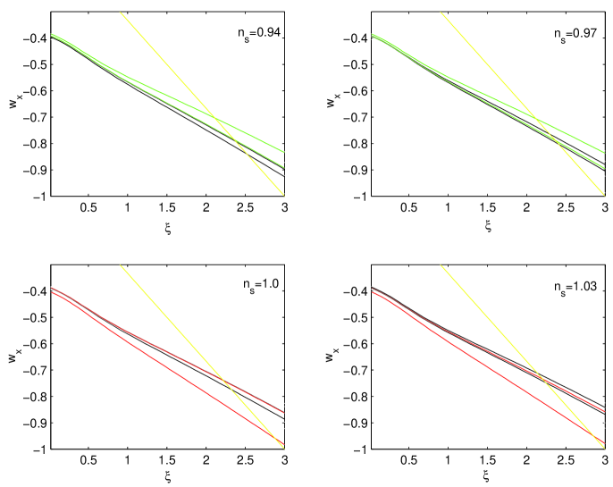
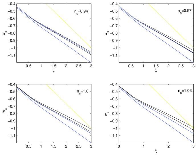
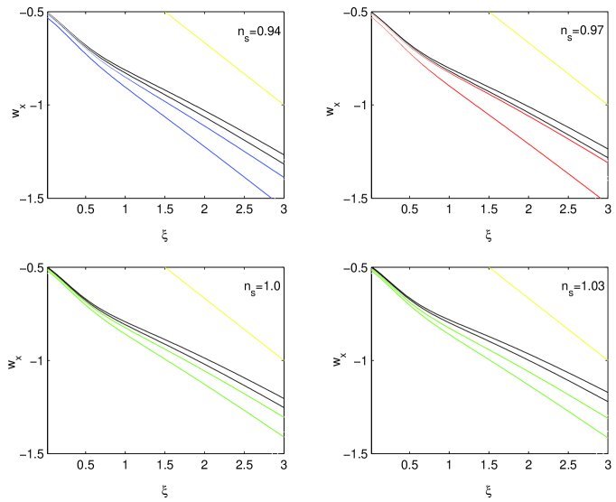
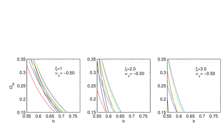
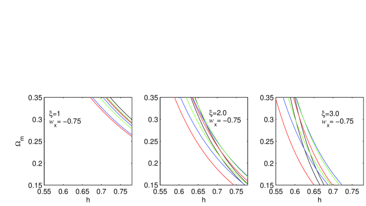
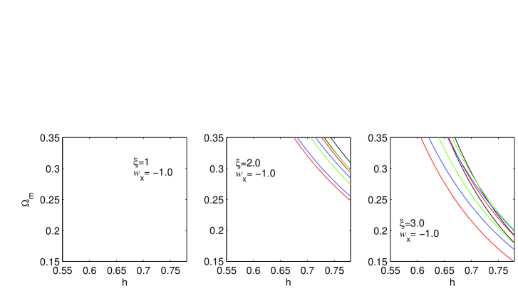
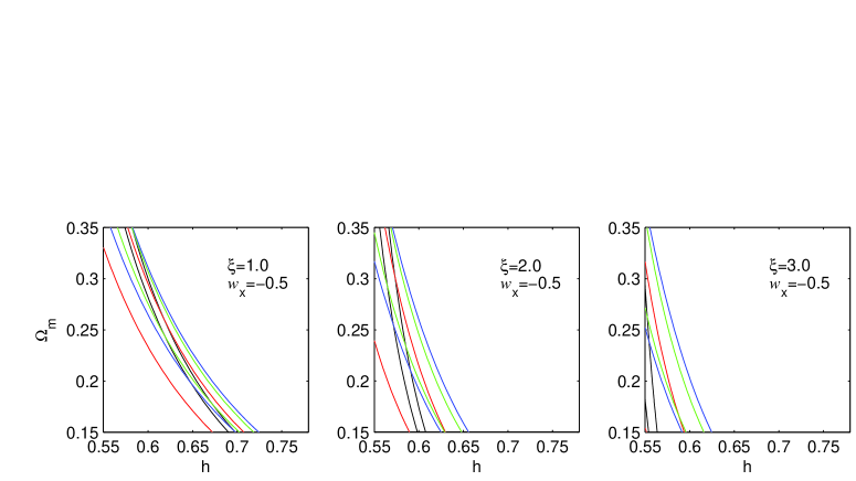
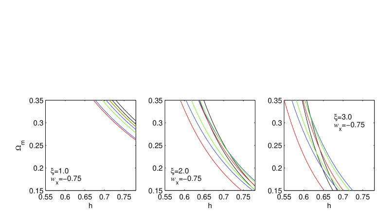
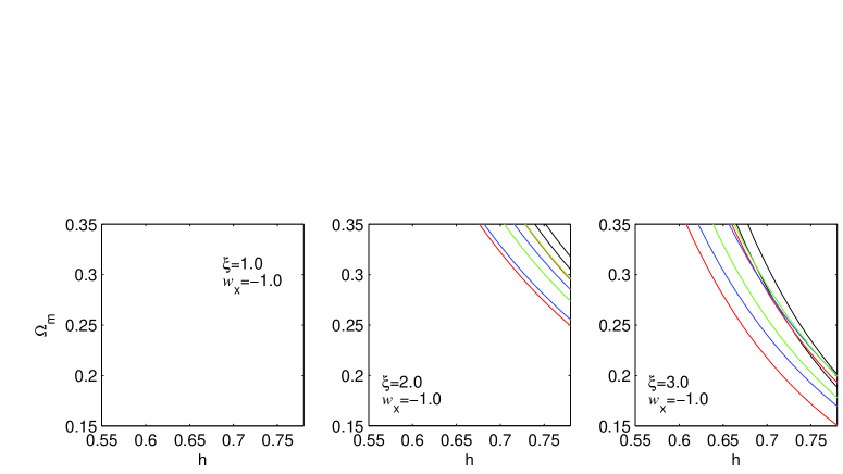
From the computation of the acoustic scale by Eq. (23), the equations for the peak shifts Eq. (18), and the fitting formulae in the Appendix, we look for the combination of the model parameters that are consistent with the observational bounds. We have plotted the contours consistent with the bounds of the first three acoustic peaks and the first trough corresponding to the WMAP and BOOMERanG data given by Eqs. (19) and (20) in the $\xi-w_{x}$ parameter space for different values of $n_{s}$ and $\Omega_{m0}$. The investigated cosmological parameter space is given by $(n_{s},h,\omega_{b},\Omega_{m})$. Throughout this paper, we have neglected the contribution from the spatial curvature and massive neutrinos. We have also neglected the contributions from gravitational waves in the initial fluctuations. Because of the rather tight WMAP constraint on $\omega_{b},(\omega_{b}=0.0224\pm 0.0009$ wmap ), we have assumed $\omega_{b}=0.0224$ in our calculations. To have a clear idea of the dependence on the parameters we have drawn two different types of plots. The first three figures show the $\xi-w_{x}$ parameter space for a particular value of $h$($=0.71$) and different values of $n_{s}$ and $\Omega_{m0}$. The next two figures depict the $\Omega_{m0}-h$ parameter space for different values of $n_{s}$, $\xi$ and $w_{x}$.

As already mentioned, we have assumed in the general outline of Sec.2 that the entire matter component, including the baryons, takes part in the interaction with the dark energy. We have also investigated the case where only the non–baryonic matter part is coupled to the dark energy, while the baryonic energy density is locally conserved. The resulting plots do not depend on these different ways to implement the interaction.

In figure 1, we have plotted the contours corresponding to the bounds of the first three peaks and the first dip (Eqs. (19) and (20)) in the $\xi-w_{x}$ parameter space with $h=0.71$ and $\Omega_{m0}=0.2$ for different values of $n_{s}$. Figures 2 and 3 represent similar contours with same $h$ and $n_{s}$ but different $\Omega_{m0}$ (0.3 and 0.4, respectively). To facilitate the analysis, all these figures show the non–interaction line, $\xi+3w_{x}=0$. It is apparent that the interaction is severely restricted by the CMB data. And simultaneously it is very interesting to notice that in Figs 2 and 3 the line $\xi+3w_{x}=0$ is clearly outside the allowed CMB regions which implies that with the assumed priors ($h=0.71$ and the mentioned value of $n_{s}$ and $\Omega_{m0}$) there is no parameter space at all consistent with a noninteracting cosmology, including the $\Lambda$CDM model.

Since the above important conclusion depends crucially on the priors chosen, we investigate the same models in a different parameter space. Figure 4 depicts the contours for the same peaks and dips in the $\Omega_{m0}-h$ parameter space with $n_{s}=0.97$ and with three different values of $\xi$ and $w_{x}$. We have chosen the values of $\xi$ as $1.0,2.0,3.0$. The higher the value of $\xi$, the more acute the coincidence problem. For $w_{x}$ we have chosen $-0.5,-0.75,-1.0$. Of course, for $\xi=3.0$ and $w_{x}=-1.0$ the model collapses to the $\Lambda$CDM model. Figure 5 represents the same contour as figure 4 with $n_{s}=1.0$ and the same values for $\xi$ and $w_{x}$.

IV Discussion

We have investigated the constraints imposed by the observed positions of the peaks of the CMB anisotropy spectrum -as witnessed by WMAP and the BOOMERanG experiments wmap , boom -, on the non–standard scaling interacting cosmology $\xi+3w_{x}\neq 0$ model scaling . The most important consequence of our analysis is that the non–standard scaling interacting cosmology shows good consistency with the observational bounds for a variety of parameter combinations. The parameter space favoured by the CMB is larger for interacting cosmological models than for noninteracting ones.

In Fig.1, for $\Omega_{m0}=0.2$, the CMB data suggests a constrained parameter space for all the four values of $n_{s}$, whereas in Fig.2, for $\Omega_{m0}=0.3$, we get an allowed region only for $n_{s}\leq 0.97$. In Fig 3, for $\Omega_{m0}=0.4$, we do not have an admissible parameter space at all. In Figs. 1 and 2, $w_{x}$ varies in the limits $-0.38>w_{x}>-1.08$ over the entire range of $\xi(0\leq\xi\leq 3)$. Thus, from the whole set of figures it is rather obvious that the scaling interacting model favours lower value of $n_{s}$ and a moderate range of values for $\Omega_{m0}$. On the other hand, the noninteracting model satisfies the parameter space bounded by CMB data only in Fig 1., i.e, for $\Omega_{m0}=0.2$. In figures 2 and 3 the noninteraction line stays well beyond the reach of the parameter space allowed by the CMB data. This includes the concordance $\Lambda$CDM model as well. Thus, the scaling model is better consistent with the CMB data and it is compatible with a larger parameter space than the noninteracting standard model.

It is worthy of note that for $\xi<1$, the region bounded by the contours of Figs. 1, 2 and 3 reduces practically to a line. For the stationary solution with no coincidence problem, $\xi\simeq 0$, we practically get a particular value for $w_{x}$ satisfied by the bounds of WMAP and BOOMERanG data. This value of $w_{x}$ varies only with $\Omega_{m0}$ -between $w_{x}\simeq-0.38$, when $\Omega_{m0}=0.2$, and $w_{x}\simeq-0.52$, when $\Omega_{m0}=0.4$. (It should be borne in mind that claims according to which observations imply that $w_{x}<-0.87$ melchiorri are based in non–interacting cosmologies).

As mentioned above in figures 1, 2 and 3, the constrained region crucially depends on $h$ and $n_{s}$. To make this clear, we present in Figs.4 and 5 contours in the $\Omega_{m0}-h$ parameter space for the same $\xi~{}{\rm and}~{}w_{x}$ but for different values of $n_{s}(0.97,1.0)$. From these plots it becomes also apparent that for a lower value of $\xi$, i.e., for a less severe coincidence problem, we have an admissible $\Omega_{m0}-h$ parameter space for higher values (lower amounts) of the equation of state parameter $w_{x}$. For example in the first column of panels in Figs. 4 and 5 (for $\xi=1.0$) we have an allowed parameter space for $w_{x}=-0.50$ only, for $w_{x}=-0.75$ there is no admissible space and for $w_{x}=-1.0$ the contours go beyond the range of the parameter space chosen. Similarly, as the coincidence problem becomes more acute, i.e., as $\xi$ grows, lower values (higher amounts) of $w_{{}_{x}}$ become more favoured. This implies that thanks to the interaction the dark energy pressure becomes less negative. The bottom-right panel in both figures corresponds to the $\Lambda$CDM model $(\xi=3.0~{}{\rm and}~{}w_{x}=-1.0)$. For the panel in Fig. 4 representing the $\Lambda$CDM model the CMB bounds are satisfied for $0.19<\Omega_{m0}<0.3$ and $h\geq 0.68$, while for the corresponding panel representing the $\Lambda$CDM model in Fig. 5, the bounds are satisfied only for $h>0.72$ and $\Omega_{m0}<0.22$. This depicts that $\Lambda$CDM favours low $n_{s}$ values. This result seems quite consistent with that of Ref. card .

After the recent high redshift SNIa data tonry ; barris lending additional support to an accelerating universe picture, and with further strings of observations (like those from the SNAP satellite) yet to come, one major worry of the community is placed on the nature of dark energy paris . In this respect, a scaling solution of the type $\rho_{m}/\rho_{x}=r_{0}(a_{0}/a)^{\xi}$ appears to be a quite promising tool for analyzing the relationship between the two forms of energy dominating our present Universe. And with the available constraints from WMAP and BOOMERanG experiments, we can certainly conclude that interacting cosmological models $(\xi+3w_{x}\neq 0)$ may well compete with the “concordance” $\Lambda$CDM model, they seem even to be favoured when compared to the latter one.

While the present cosmological data are insufficient to discriminate between these models, it is to be hoped that future observations of high redshift SNIa as well as other complementary data (from galaxy clusters evolution and lensing effects) will decisively help to break the degeneracy.

Appendix

For completeness, we put together here the formulas used in our search for parameter space. These fitting formulae are quoted from the cited literature doran2 .

We assume the standard recombination history and define the redshift $z_{ls}$ of decoupling as the redshift at which the optical depth of Thompson scattering is unity. A useful fitting formula for $z_{ls}$ is given by param :

$$z_{ls}=1048[1+0.00124\omega_{b}^{-0.738}][1+g_{1}\omega_{m}^{g_{2}}],$$ (24)

where

$$g_{1}=0.0783\omega_{b}^{-0.238}[1+39.5\omega_{b}^{0.763}]^{-1},\;\;\;g_{2}=0.56[1+21.1\omega_{b}^{1.81}]^{-1},$$

$\omega_{b}\equiv\Omega_{b}h^{2}$ and $\omega_{m}\equiv\Omega_{m}h^{2}$.

The ratio of radiation to matter at last scattering is

$$r_{ls}=\rho_{r}(z_{ls})/\rho_{m}(z_{ls})=0.0416\omega_{m}^{-1}\left(z_{ls}/10^{3}\right).$$ (25)

The overall phase shift $\bar{\varphi}$ (which is the phase shift of the first peak) is parametrized by the formula

$$\bar{\varphi}=(1.466-0.466n_{s})\left[a_{1}r_{{ls}}^{a_{2}}+0.291\bar{\Omega}_{ls}^{d}\right],$$ (26)

where $a_{1}$ and $a_{2}$ are given by

$$a_{1} = 0.286+0.626~{}\omega_{b}\,,$$ (27)

$$a_{2} = 0.1786-6.308~{}\omega_{b}+174.9~{}\omega_{b}^{2}-1168~{}\omega_{b}^{3}.$$ (28)

The relative shift of the second peak $(\delta\phi_{2})$ is given by

$$\delta\varphi_{2}=c_{0}-c_{1}r_{ls}-c_{2}r_{ls}^{-c_{3}}+0.05\,(n_{s}-1),$$ (29)

with

$$c_{0} = -0.1+\left(0.213-0.123\bar{\Omega}_{ls}^{d}\right)$$ (31)

$$\times\exp\left\{-\left(52-63.6\bar{\Omega}_{ls}^{d}\right)\omega_{b}\right\}$$

$$c_{1} = 0.063\,\exp\{-3500~{}\omega_{b}^{2}\}+0.015$$ (32)

$$c_{2} = 6\times 10^{-6}+0.137\left(\omega_{b}-0.07\right)^{2}$$ (33)

$$c_{3} = 0.8+2.3\bar{\Omega}_{ls}^{d}+\left(70-126\bar{\Omega}_{ls}^{d}\right)\omega_{b}.$$ (34)

For the third peak we have,

$$\delta\varphi_{3}=10-d_{1}r_{ls}^{d_{2}}+0.08\,(n_{s}-1),$$ (35)

with

$$d_{1} = 9.97+\left(3.3-3\bar{\Omega}_{ls}^{d}\right)\omega_{b}$$ (36)

$$d_{2} = 0.0016-0.0067\bar{\Omega}_{ls}^{d}+\left(0.196-0.22\bar{\Omega}_{ls}^{d}\right)\omega_{b}$$ (37)

$$+\frac{(2.25+2.77\bar{\Omega}_{ls}^{d})\times 10^{-5}}{\omega_{b}}.$$

The relative shift of the first trough is given by

$$\delta\varphi_{3/2}=b_{0}+b_{1}r_{ls}^{1/3}\exp(b_{2}r_{ls})+0.158(n_{s}-1)~{}$$ (38)

with

$$b_{0} = -0.086-0.079{\bar{\Omega}}_{ls}^{d}-\left(2.22-18.1{\bar{\Omega}}^{d}_{ls}\right)\omega_{b}$$

$$-\left(140+403{\bar{\Omega}}^{d}_{ls}\right)\omega_{b}^{2}~{},$$

$$b_{1} = 0.39-0.98{\bar{\Omega}}^{d}_{ls}-\left(18.1-29.2{\bar{\Omega}}_{d}^{ls}\right)\omega_{b}$$ (39)

$$+440\omega_{b}^{2},$$

$$b_{2} = -0.57-3.8\exp({-2365\omega_{b}^{2}})~{}.$$ (40)

The overall shifts for the second and the third peaks and for the first trough are $\bar{\phi}+\delta\phi_{2}$, $\bar{\phi}+\delta\phi_{3}$ and $\bar{\phi}+\delta\phi_{3/2}$, respectively. In the above expressions, $\bar{\Omega}_{ls}^{d}$ is the average fraction of dark energy before last scattering, which is negligibly small in the cases discussed here.

Figure 1: Contour Plots of the first three Doppler peaks and the first trough location in the $(\xi,w_{x})$ plane with $\Omega_{m0}=0.2$ and $h=0.71$ for different values of $n_{s}$. Black, red, blue and green lines correspond to the observational bounds on the first, second, third peaks and the first trough, respectively (given in equations (20) and (21)). The upper line corresponds to the non-interacting case $(\xi+3w_{x}=0)$. To avoid confusion, we plot only the contours relevant for the admissible range. For each panel contours not shown are consistent with this range.

Figure 2: Same as Figure 1 with $h=0.71$ but $\Omega_{m0}=0.3$.

Figure 3: Same as Figure 1 with $h=0.71$ but $\Omega_{m0}=0.4$.

Figure 4: Contour Plots of the first three Doppler peaks and the first trough location in the $(\Omega_{m0},h)$ plane with $n_{s}=0.97$ and for different values of $\xi$ and $w_{x}$. Black, red, blue and green lines correspond to the observational bounds on the first, second, third peaks and the first trough,respectively (given in equations (20) and (21)).

Figure 5: Same as Figure 4 but with $n_{s}=1.0$ and different values of $\xi$ and $w_{x}$.

References

- (1) Bernadis, P. De. et al., 2000, Nature 404, 955; Hanany, S. et al., 2000, Astrophys. J. 545, L5; Balbi, A. et al., 2000, Astrophys. J. 545, L1; ibid., 2001 558 L145; Perlmutter, S. et al., 1997, Astrophys. J. 483, 565; Perlmutter, S. et al., 1998, Nature, 391, 51; Garnavich, P.M. et al., 1998, Astrophys. J. 493, L53; Riess, A.G. 1998, Astron. J. 116, 1009.
- (2) Caldwell, R.R., Dave, R. and Steinhardt, P.J., 1998, Phys. Rev. Lett. 80, 1582; Peebles, P.J.E. and Ratra, B., 1988, Astrophys. J. 325, L17; Steinhardt, P.J., Wang, L., and Zlatev, I., 1999, Phys. Rev. Lett. 59, 123504; Uzan, J.P., 1999, Phys. Rev. D 59, 123510; Amendola, L. 2000, Phys. Rev. D, 62, 043511; Sen, S. and Sen, A.A., 2001a, Phys. Rev. D 63, 124006; Sen, A.A. and Sen, S. 2001b, Mod. Phys. Lett. A, 16, 1303; Banerjee, N. and Pavón, D., 2001, Phys. Rev. D 63, 043504; Banerjee, N. and Pavón, D., 2001, Class. Quantum Grav. 18, 593.
- (3) Steinhardt, P.J., in Critical Problems in Physics, edited by Fitch, V.L. and Marlow, D.R. (Princeton University Press, Princeton, N.J., 1997).
- (4) Zlatev, I., Wang, L., and Steinhardt, P.J., 1999, Phys. Rev. Lett. 82, 896; Zlatev,I. and Steinhardt, P.J., 1999, Phys. Lett. B 459, 570; Arkani–Hamed, N., Hall, L.J., Kolda, C.F., and Murayama, H., 2000, Phys. Rev. Lett. 85, 4434; Griest, K., 2002, Phys. Rev. D 66, 123501; Cohen, I. astro-ph/0304029; Pietroni, M., 2003, Phys. Rev. D 67, 103523.
- (5) Chimento, L.P., Jakubi, A.S., Pavón, D. and Zimdahl, W., 2003, Phys. Rev. D 67, 083513; Chimento, L.P., Jakubi, A.S. and Pavón, D., 2003, Phys. Rev. D 67, 087302.
- (6) Dalal, N., Abazajian, K., Jenkins, E. and Manohar, A.V., 2001, Phys. Rev. Lett. 87, 141302.
- (7) Zimdahl, W. and Pavón, D., 2003, Gen. Rel. Grav. 35, 413.
- (8) Zimdahl, W., Pavón, D. and Chimento, L.P., 2001, Phys. Lett. B 521, 133.
- (9) Perlmutter, S. et al. 1999, Astrophys. J., 517, 565;
- (10) Spergel, D.N. et al., 2003 Astrophys. J. Suppl. 148, 175; Page, L. et al., LANL preprint astro-ph/0302220, Astrophys. J. (in the press).
- (11) Ruhl,J.E. et al.,2003, Astrophys. J. 599, 786.
- (12) Sen, A.A. and Sen, S., 2003, Phys.Rev.D 68, 023513; Sen, S. and Sen,A.A., 2003, Astrophys. J, 588, 1; Bento, M.C., Bertolami, O., and Sen,A.A., 2003, Phys. Lett. B 575, 172.
- (13) Hu, W., Fukugita. M., Zaldarriaga, M. and Tegmark., M., 2001, Astrophys. J. 549, 669.
- (14) Doran, M., Lilley, M.J., Schwindt, J. and Wetterich, C., 2001, Astrophys. J. 559, 501.
- (15) Doran, M. and Lilley,M.J., 2002, Mon. Not. Roy. Astron. Soc. 330 965.
- (16) Tonry, J.L. et al., 2003, Astrophys. J. 594, 1
- (17) Barris, B.J. et al., 2003 astro-ph/0310843, Astrophys. J. (in the press).
- (18) Melchiorri, A. and Ödman, C.J., 2003, Phys. Rev. D 67, 081302.
- (19) Brax, P., Martin, J. and Uzan, J.P. (editors) Proceedings of the IAP Conference “On the Nature of Dark Energy” (Frontier Group, Paris, 2003).
- (20) Durrer, R., Novosyadlyl, D. and Apunevych, S., 2003, Astrophys. J. 583, 33.