The Environmental Dependence of the Relations between Stellar Mass, Structure, Star Formation and Nuclear Activity in Galaxies
Guinevere Kauffmann¹, Simon D.M. White¹, Timothy M. Heckman², Brice Ménard^3,1, Jarle Brinchmann^1,4, Stéphane Charlot^1,5, Christy Tremonti⁶, Jon Brinkmann^7
1Max-Planck Institut für Astrophysik, D-85748 Garching, Germany
²Department of Physics and Astronomy, Johns Hopkins University, Baltimore, MD 21218
³Institute for Advanced Study, Einstein Drive, Princeton, NJ 08540
⁴ Centro de Astrofisica da Universidade do Porto, Rua das Estrelas, 4150-762 Porto, Portugal
⁵ Institut d’Astrophysique du CNRS, 98 bis Boulevard Arago, F-75014 Paris, France
⁶ Steward Observatory, 933 North Cherry Ave, Tuscon, AZ 85721
⁷ Apache Point Observatory, P.O. Box 59, Sunspot, NM 88349

We use a complete sample of galaxies drawn from the Sloan Digital Sky Survey (SDSS) to study how structure, star formation and nuclear activity depend on local density and on stellar mass. Local density is estimated by counting galaxies above a fixed absolute magnitude limit within cylinders 2 Mpc in projected radius and $\pm$500 km s^-1 in depth. The stellar mass distribution of galaxies shifts by almost a factor of two towards higher masses between low and high density regions. At fixed stellar mass both star formation and nuclear activity depend strongly on local density, while structural parameters such as size and concentration are almost independent of it. Only for low mass galaxies ($M_{*}<3\times 10^{10}M_{\odot}$) do we find a weak shift towards greater concentration and compactness in the highest density regions. The galaxy property most sensitive to environment is specific star formation rate. For galaxies with stellar masses in the range $10^{10}-3\times 10^{10}M_{\odot}$, the median SFR/M_∗ decreases by more than a factor of 10 as the population shifts from predominantly star-forming at low densities to predominantly inactive at high densities. This decrease is less marked, but still significant for high mass galaxies. Galaxy properties that are associated with star formation correlate strongly with local density. At fixed stellar mass twice as many galaxies host AGN with strong [OIII] emission in low density regions as in high. Massive galaxies in low-density environments also contain more dust. To gain insight into the processes that shut down star formation, we analyze correlations between spectroscopic indicators that probe the SFH on different timescales: the 4000 Å break strength, the Balmer-absorption index H$\delta_{A}$, and the specific star formation rate SFR/$M_{*}$. The correlations between these indicators do not depend on environment, suggesting that the decrease in star formation activity in dense environments occurs over long ($>1$ Gyr) timescales. Since structure does not depend on environment for galaxies with masses greater than $3\times 10^{10}M_{\odot}$, the trends in recent star formation history (SFH), dust and nuclear activity in these systems cannot be driven by processes that alter structure, for example mergers or harrassment. The SFH-density correlation is strongest for small scale estimates of local density. We see no evidence that star formation history depends on environment more than 1 Mpc from a galaxy. Finally, we highlight a striking similarity between the changes in the galaxy population as a function of density and as a function of redshift. We use mock catalogues derived from N-body simulations to explain how this may be understood.

Keywords: galaxies:formation,evolution; galaxies: stellar content

1 Introduction

One of the most fundamental correlations between the properties of galaxies in the local Universe is the so-called morphology-density relation. This relation was first quantified by Oemler (1974) and Dressler (1980) who showed that star-forming, disk-dominated galaxies reside in lower density regions of the Universe than inactive elliptical galaxies. The standard morphological classification scheme mixes elements that depend on the structure of a galaxy (disk-to-bulge ratio, concentration, surface density) with elements related to its recent star formation history (dust-lanes, spiral arm strength). It is by no means obvious that these two elements should depend on environment in the same way. The physical orgin of the morphology density relation is still a subject of debate. Much of the argument centres on whether the relation arises early on during the formation of the object (the so-called ‘nature’ hypothesis), or whether it is caused by density-driven evolution (the ‘nurture’ scenario).

There are many different physical processes that could in principle play a role in driving the morphology-density relation. Mergers or tidal interactions can destroy galactic disks and convert spiral and irregular galaxies into bulge-dominated ellipticals and S0s (Toomre & Toomre 1972; Farouki & Shapiro 1981). Mergers operate most efficiently in galaxy groups. In clusters merging cross-sections are low, but galaxies may still be affected by the cumulative effect of many weaker encounters (Richstone 1976; Moore et al 1996). Interactions with the dense intracluster gas may also strip away the interstellar medium of a galaxy and cause a strong reduction in its star formation rate (Gunn & Gott 1972). Finally, gas cooling processes are also strongly dependent on environment. In dark matter halos with low masses, infalling cold gas is never shock-heated and will collapse directly onto the galaxy. In high mass halos, collapsing gas is first heated to the halo virial temperature by shocks; it then remains pressure-supported and in quasi-static equilibrium while it cools by radiative processes (White & Frenk 1991; Birnboim & Dekel 2003).

Disentangling the processes responsible for the observed correlations has proved to be a difficult task. However, the subject has received much impetus from the completion of large spectroscopic and photometric surveys of nearby galaxies. There have been many recent papers analyzing trends in galaxy colours and emission line equivalent widths as a function of local galaxy density and as a function of distance from the centres of clusters. These studies indicate that the correlation between the star formation history of a galaxy and its environment extends to low densities and to large clustercentric radii (e.g. Kodama et al 2001; Gomez et al 2003; Lewis et al 2002; Pimbblet et al 2002; Balogh et al 2003). This suggests that the morphology-density relation is not driven by processes that operate only in extreme environments, such as the centres of rich clusters.

There have also been studies of the relative strength with which different galaxy properties correlate with density. These indicate that galaxy colour is the property most tightly linked to environment. Galaxy luminosity also depends on environment, but at fixed luminosity, the structural parameters and surface brightnesses of galaxies depend only weakly on density (Blanton et al 2003c). These results suggest that processes such as merging or harrassment, do not drive the primary correlation between colour and density. Other recent studies of the effect of environment on galaxy properties using large galaxy surveys include the study of the morphology-density relation by Goto et al (2003a) and the study of the frequency of AGN as a function of environment by Miller et al (2003).

Over the past few years, we have been developing new methods for constraining the physical properties of galaxies using the wealth of information contained in the high signal-to-noise, high-resolution galaxy spectra from the Sloan Digital Sky Survey (hereafter SDSS; York et al 2000; Stoughton et al 2002 Abazaijan et al 2003). We have applied these methods to a sample of $\sim$ 100,000 galaxies in the SDSS Data Release One (DR1). We used two stellar absorption line indicators, the 4000 Å break strength D_n(4000) and the Balmer absorption line index H$\delta_{A}$, to constrain the mean stellar age and star formation history of each galaxy. A comparison with broad band magnitudes then yields estimates of dust attenuation and of stellar mass. Our methodology for deriving stellar mass, dust attenuation strength and burst mass fraction is described in Kauffmann et al (2003a;hereafter Paper I ). We have also used the emission lines in the spectra to identify galaxies with active nuclei (AGN). We then use the comined population synthesis and photo-ionization models of Charlot & Longhetti (2001) to derive gas-phase metallicity, star formation rate, ionization parameter, dust-to-gas ratio and extinction for emission-line galaxies without AGN. Results using physical parameters derived from both absorption and emission lines have been presented in Kauffmann et al (2003b,c), Brinchmann et al (2004) and Tremonti et al (2004).

Our studies have revealed that many of the physical properties of galaxies are very strongly correlated. Almost all galaxy properties depend strongly on stellar mass. Massive galaxies have old stellar ages, high mass-to-light ratios, low star formation rates and little dust attenuation They also have high concentrations and stellar surface mass densities and they frequently host AGN. Low mass galaxies have young stellar ages, low mass-to-light ratios and are usually actively forming stars at the present day. They have low concentrations and stellar surface mass densities and they almost never contain active nuclei. There is also a tight relation between stellar mass and gas-phase metallicity for the emission line galaxies in the sample. Although many of these correlations were already known from previous analyses, the very large number of galaxies in the SDSS sample has allowed us to quantify the distribution of different galaxy properties as a function of mass. Our analysis has also revealed that there is a characteristic stellar mass ($\sim 3\times 10^{10}M_{\odot}$) where many of these properties appear to change very rapidly.

In this paper, we attempt to gain more insight into the nature of these relations by studying how they depend on environment. According to the standard cosmological paradigm , structure in the present-day Universe formed through a process of hierarchical clustering, with small structures merging to form progressively larger ones. The theory predicts that density fluctuations on galaxy scales collapsed earlier in regions that are currently overdense. Galaxies in high density regions of the Universe such as galaxy clusters are thus more ‘evolved’ than galaxies in low density regions or voids. As we have discussed, not only did galaxies in dense regions “form” earlier, but they have also been more subject to processes such as stripping and harrassment that operate preferentially in such environments. By studying how the relations between different galaxy properties vary with density, we hope to deduce whether these relations were established early on when the galaxy first assembled (nature) or whether they are the end product of a set of physical processes that have operated over the whole history of the Universe (nurture).

Our paper is structured as follows: Section 2 reviews the properties of the galaxy sample. Section 3 discusses our methods for characterizing the environments of the galaxies in our sample. Section 4 re-introduces the stellar mass partition function of Paper I and discusses how it varies with environment. In section 5, we discuss how the correlations between different galaxy properties depend on density. In section 6, we attempt to place constraints on the scale-dependence of the environmental effect. Finally in section 7, we interpret our results in the light of modern theories of structure formation.

2 Review of the Spectroscopic Sample of Galaxies

The on-going Sloan Digital Sky Survey is using a dedicated 2.5-meter wide-field telescope at the Apache Point Observatory to conduct an imaging and spectroscopic survey of about a quarter of the sky. The imaging is conducted in the $u$, $g$, $r$, $i$, and $z$ bands (Gunn et al. 1998; Hogg et al. 2001; Fukugita et al. 1996; Smith et. al. 2002), and spectra are obtained with a pair of multi-fiber spectrographs. When the survey is complete, spectra will have been obtained for nearly 10⁶ galaxies and 10⁵ QSOs selected from the imaging data. The results in this paper are based on spectra of $\sim$122,000 galaxies with $14.5<r<17.77$ contained in the the SDSS Data Release One (DR1). These data were made publically available in 2003. Details on the spectroscopic target selection for the “main” galaxy sample can be found in Strauss et al. (2002) and description of the tiling algorithm is given in Blanton et al (2002). The reader is referred to Pier et al (2003) for details about the astrometric calibration.

The spectra are obtained through 3 arcsec diameter fibers. At the median redshift, the spectra cover the rest-frame wavelength range from $\sim$3500 to 8500 Å with a spectral resolution $R\sim$ 2000 ($\sigma$${}_{instr}\sim$ 65 km/s). The spectra are spectrophotometrically calibrated through observations of F stars in each 3-degree field. By design, the spectra are well-suited to the determinations of the principal properties of the stars and ionized gas in galaxies. The spectral indicators (primarily the 4000 Å  break and the H$\delta_{A}$ index) and the emission line fluxes used to determine the star formation rates analyzed in this paper are calculated using a special-purpose code described in detail in Tremonti et al (2004, in preparation). A detailed description of the galaxy sample and the methodology used to derive parameters such as stellar mass and dust attenuation strength can be found in Paper I. A description of the methods for deriving physical parameters from the emission line measurements can be found in Brinchmann et al (2003).

The SDSS imaging data provide the basic structural parameters that are used in this analysis. The $z$-band absolute magnitude, combined with our estimated values of M/L and dust attenuation $A_{z}$ yield the stellar mass ($M_{*}$). The half-light radius in the $z$-band and the stellar mass yield the effective stellar surface mass-density ($\mu_{*}=M_{*}/2\pi r_{50,z}^{2}$). As a proxy for Hubble type we use the SDSS “concentration” parameter $C$, which is defined as the ratio of the radii enclosing 90% and 50% of the galaxy light in the $r$ band (see Stoughton et al. 2002). Strateva et al. (2001) find that galaxies with $C>$ 2.6 are mostly early-type galaxies (E, S0 and Sa), whereas spirals and irregulars have 2.0 $<C<$ 2.6. Throughout this paper, we have assumed a cosmology with $\Omega=0.3$, $\Lambda=0.7$ and H₀= 70 km s^-1 Mpc^-1.

3 The Definition of the Density Estimator

Two main approaches have been used to characterize the environments of galaxies in redshift surveys. One is to assign galaxies to groups or to clusters. If a group contains a sufficient number of galaxies with measured redshifts, its velocity dispersion can be computed and a correspondence can be made with a virialized dark matter halo of some circular velocity or mass. The main drawback of this approach is that there is no set procedure for finding groups or clusters. Many different methods have been proposed and each must be tested and calibrated using mock catalogues drawn from N-body simulations (Nolthenius & White 1987; see Marinoni et al 2002 and Miller et al 2004 for more recent discussions). In addition, only a relatively small fraction of galaxies in a flux-limited sample can be assigned to a group or cluster. Galaxies with only a few close neighbours are generally excluded from analysis.

In the second approach, a local density is estimated for each galaxy in the sample. Following the early work of Dressler (1980), many authors have estimated density using the projected distance to the $n$th nearest spectroscopically-observed neighbour, with $n$ in the range $3-10$ (e.g. Hashimoto et al 1998; Gomez et al 2003; Lewis et al 2003; Tanaka et al 2003). Because the density of galaxies varies with distance in a magnitude-limited survey, most such analyses are restricted to volume-limited sub-samples of the full survey.

Other authors have estimated density using galaxy counts within fixed metric apertures. For example, recent studies of galaxy properties as a function of density in the SDSS survey (Blanton et al (2003a,b) and Hogg et al (2003a,b)) have used a variety of estimators, including counts of galaxies in the spectroscopic sample within spheres or cylinders 8 $h^{-1}$ Mpc in radius and counts in the imaging data smoothed over scales of 1 $h^{-1}$Mpc.

In this paper, we follow an approach similar to that of Blanton, Hogg and collaborators. We calculate local density using galaxy counts to a fixed absolute magnitude inside a fixed volume. Our choice of “target” galaxies and of the volume within which we evaluate the counts around them are motivated by two important considerations:

1. We wish to study galaxy properties over a large range in stellar mass and hence over a large range in absolute magnitude. Our target sample must therefore extend to low redshifts in order to include low mass galaxies.

2. We wish to study not only how galaxy properties such as mass or star formation history correlate with density, but also how the relations between these properties change with environment. We thus require a large sample of targets.

Together these considerations mandate a density estimator that can be applied uniformly over a reasonably large range in redshift. As discussed by Blanton et al (2003a), signal-to-noise considerations favour galaxy counts calculated within large volumes. Theoretical considerations, however, suggest that one should estimate the local density within a small volume. As shown by Lemson & Kauffmann (1999), the only property of a dark matter halo that is strongly correlated with environment on large scales is mass. Properties such as spin parameter, concentration and formation time show almost no dependence on the surrounding dark matter density or on the external tidal field. The formation path and the merging history of a dark matter halo (and so presumably of the galaxies within it) depends on its present-day virial mass but not on its larger scale environment. Fluctuations on galaxy-scales will collapse earlier in those regions of the Universe that end up inside massive halos at $z=0$ (e.g. Bower 1991; Lacey & Cole 1993). From a theoretical standpoint, it is thus natural to expect that galaxy properties should correlate most strongly with densities evaluated on scales comparable to the virial radii of typical halos at the present day ($\sim$ 1 h^-1 Mpc).

The sample of target galaxies used in this paper was selected to have apparent magnitudes in the range $14.5<r<17.77$ and redshifts in the range $0.03<z<0.1$. Galaxies down to a limiting $r$-band magnitude of $-18.1$ are thus included in the sample. In Paper I we showed that the maximum $r$-band stellar mass-to-light ratio for galaxies of this absolute magnitude is $\sim 1.5$. This means that our sample should be complete down to stellar masses of $2\times 10^{9}$ M_⊙.

We have constructed a volume-limited sample of “tracer” galaxies that we use to evaluate the density around every target. We have used the photometric galaxies in DR1 that overlap with the spectroscopic survey, namely the stripes 9-12, 33-36, 76, 82 and 86. In practice, we first select target galaxies that lie sufficiently far away from the nearest survey boundary or missing fields. This reduces the number of usable target objects, but it allows us to work with a density estimator that is well defined for all target galaxies and that does not suffer from problems due to edge effects. We then count the number of spectroscopically-observed galaxies that are located within 2 Mpc in projected radius and $\pm 500$ km s^-1 in velocity difference from the target. We eliminate all galaxies that are predicted to be fainter than r=17.77 at $z=0.1$ (we adopt the K-corrections of Blanton et al (2002c)). We also correct for galaxies that were missed as a result of fibre collisions. This is done by counting the number of galaxies in the imaging survey with $14.5<r<17.77$ and $R_{proj}<2$ Mpc ($N_{image}$). We compare this with the number of galaxies that were targeted spectroscopically ($N_{spectro}$). We then multiply the number counts within our adopted volume by the correction factor $f_{corr}=N_{image}/N_{spectro}$ . These correction factors are generally small ($\sim$ 10-20%).

Our final sample consists of 46,892 target galaxies. The distribution of counts around our sample of targets is shown in Fig. 1. We plot the cumulative fraction of galaxies with counts less than a given value. Fig. 1 shows that only 20% of the galaxies in our sample have no neighbours. Around half have 2 or more neighbours and 10% have more than 10 neighbours. The dotted line shows the count distribution around randomly chosen points within our survey area. This gives some indication of the expected level of contamination due to chance projections. As can be seen, 76% of the randomly placed galaxies have no neighbours and only a tiny fraction have more than a few.

As a final comment, we emphasize that our choice of density estimator is a compromise based on considerations of sample size, signal-to-noise and smoothing scale. In section 6, we will restrict our analysis to low redshift galaxies and explore in more detail the effect of changing the volume within which the density is computed.

Figure 1: The cumulative fraction of galaxies with counts less than $N$ for the target sample (solid) and for a random sample (dotted).

4 Environmental Dependence of the Stellar Mass Partition Function

The study of how the clustering properties of galaxies vary as a function of luminosity, colour, spectral type and morphology has a long history and a number of different, but complementary approaches have been used in analyzing the available data.

One approach is to study how the auto-correlation function changes if galaxies are selected according to different criteria. The early work of Davis & Geller (1976) already showed that the two point function is a strong function of galaxy morphology, being steeper and having a higher amplitude on small scales for early-type galaxies than for late-types. There now appears to be a consensus that the slope of the two-point function is a strong function of the colour or the spectral type of a galaxy, with red, early-type galaxies exhibiting steeper slopes than blue, late-type galaxies (Willmer, Da Costa & Pellegrini 1998; Zehavi et al 2002; Madgwick et al 2003; Budavari et al 2003). If galaxies are split according to luminosity, then the correlation length increases for brighter galaxies, but the slope remains approximately constant (Loveday et al 1995; Norberg et al 2001; Zehavi et al 2002).

There have also been a number of studies addressing how the galaxy luminosity function changes as a function of environment. Most authors seem to agree that the characteristic magnitude $M_{*}$ does vary weakly with density. It appears to be somewhat brighter in clusters than in the general field (Balogh et al 2001; De Propris et al 2003) and to be fainter in voids (Hoyle et al 2003). This is in qualitative agreement with correlation function studies described above. There is, however, no clear consensus on whether the faint-end slope of the luminosity function depends on environment.

Finally, there have been many recent papers analyzing how galaxy properties such as colours, luminosities, structural parameters and star formation rates correlate with local density (e.g. Blanton et al 2003a,b; Hogg et al a,b; Gomez et al 2003; Balogh et al 2003; Tanaka et al 2003). Once again there is general consensus that luminous, red, non-star-forming galaxies inhabit denser regions of the Universe than faint, blue, star-forming galaxies. In their most recent paper, Blanton et al (2003b) find that galaxy colour is the property that is most tightly related to local environment. They also find that the structural properties of galaxies are less closely related to environment than their masses and star formation histories.

In this section, we adopt yet another approach. In Paper I, we computed how different kinds of galaxies contribute to the total stellar mass budget of the local Universe. Each galaxy in our sample was given a weight equal to the inverse of the volume in which it could have been detected. We then calculated the fraction of the total stellar mass contained in galaxies as a function of their stellar mass, D_n(4000), $g-r$ colour, size, concentration index and surface mass density. We found that most of the stellar mass in the nearby Universe resides in galaxies that have stellar masses $\sim 5\times 10^{10}M_{\odot}$, half-light radii $\sim 3$ kpc and half-light surface mass densities $\sim 10^{9}M_{\odot}$ kpc^-2. The distribution of stellar mass as a function of D_n(4000) is strongly bimodal, showing a clear division between galaxies with old stellar populations and galaxies with more recent star formation.

It is interesting to investigate how the stellar mass partition functions presented in Paper I vary with environment. This is shown in Fig. 2. We have divided our sample into 5 density bins and the partition function for each bin is represented by a curve with a different colour. Cyan is for galaxies with 0 or 1 neighbour, blue is for $N_{neighb}=2-3$, green is for $N_{neighb}=4-6$, black is for $N_{neighb}=7-11$, and red is for $N_{neighb}>12$.

The first three panels of Fig. 2 show how the division of stellar mass among galaxies of different masses, concentrations and surface densities changes as a function of density. We find that galaxies in lower density environments tend to be less massive, less concentrated and less dense, but the trends are relatively weak. In contrast, the change in the distribution of stellar mass as a function of D_n(4000) or $g-r$ colour is quite dramatic. In the D_n(4000) panel, the stellar mass distribution shifts systematically from the “blue” to the “red” peak as density increases.

We also illustrate how the stellar mass is partitioned as a function of the normalized star formation rate estimated by Brinchmann et al (2003), which is defined as the present-day star formation rate (SFR) of the galaxy divided by its stellar mass $M_{*}$. In calculating this ratio for Fig. 2, both the SFR and the stellar mass are estimated for the light within the fibre aperture (see Brinchmann et al for more details). The distribution of stellar mass as a function of SFR/M_∗ shows the same bimodality as the distribution as a function of D_n(4000). In low-density regions, more than half the stellar mass resides in galaxies that are presently forming stars at a rate comparable to their past-averaged one. In high-density regions, almost all of the stellar mass resides in galaxies with very low present-day rates of star formation. (Note that the strong peak at $\log$ SFR/M${}_{*}=-11.6$ is artificial; all galaxies with very weak or undetectable star formation have been assigned values in this range).

Figure 2: The fraction of the total stellar mass in the local Universe contained in galaxies as a function of log M_∗, log $\mu_{*}$, concentration index, D_n(4000), SFR/$M_{*}$ and $g-r$ colour (k-corrected to z=0.1). The different colour lines represent the different density bins as follows: cyan, 0 or 1 neighbour; blue, 2-3 neighbours; green, 4-6 neighbours; black, 7-11 neighbours; red, more than 12 neighbours.

Figure 3: The cumulative fraction of the total stellar mass in the local Universe contained in galaxies as a function of log M_∗, log $\mu_{*}$, concentration index, D_n(4000), SFR/$M_{*}$ and $g-r$ colour. The different colour lines represent the different density bins as in Fig. 2.

In Fig. 3 we replot the distributions of Fig. 2 in cumulative form. Let us define $p(0.5)$ as the value of the parameter $p$ at a mass fraction of one half. Fig. 2 shows that $M_{*}(0.5)$ shifts by just under 0.3 dex from our lowest density bin to our highest density bin. The shift is even smaller for the stellar surface mass density $\mu_{*}$. By contrast, SFR/M_∗(0.5) shifts by more than an order of magnitude from low density to high density regions (the median value is actually too low to be measured in our highest density bins). It also useful to transform the shift into dimensionless units in order to compare results for different parameters in a uniform way. We define a shift $\Delta p$ as

$$\Delta p=\frac{\bar{p}_{red}-\bar{p}_{cyan}}{p_{all}(0.95)-p_{all}(0.05)},$$ (1)

where $\bar{p}$ is the mass-weighted mean value of parameter $p$ for galaxies in a given density bin, and $p_{all}(0.95)$ and $p_{all}(0.05)$ are the values of $p$ at mass fractions of 0.95 and 0.05 for the sample as a whole. Values of $\Delta p$ for different galaxy parameters are listed in Table 1. As can be seen, the shifts are smallest for the structural parameters $\mu_{*}$ and $C$ and largest for our star formation history indicators $g-r$, D_n(4000) and SFR/M_∗ . We thus conclude, in agreement with Blanton et al (2003b), that star-formation history is the galaxy property that is most strongly dependent on environment.

It is curious that the stellar mass partition function exhibits a clear bimodality when plotted as a function of D_n(4000) or SFR/$M_{*}$, but not when plotted as a function of $g-r$. The colours of star-forming galaxies appear to be more broadly distributed than their 4000 Å break strengths. This is because the colours of star-forming galaxies are significantly affected by dust attenuation. In Fig. 4 we show how stellar mass divides among galaxies with different amounts of attenuation. The $z$-band attenuation A_z is estimated by comparing stellar absorption line indicators with galaxy colours, as described in Paper I. As can be seen, galaxies in low density regions of the Universe typically contain more dust than galaxies in high density regions. This is not unexpected, because we have already shown that a larger fraction of the stellar mass in low-density environments is in star-forming and hence gas-rich galaxies.

Table 1: Relative shift $\Delta p$ in the mass-weighted mean value of the parameter from the lowest density (cyan) to the highest density bin (red).

Parameter	$\Delta p$
log $M_{*}$	0.164
log $\mu_{*}$	0.126
C	0.124
Dn(4000)	0.252
SFR/$M_{*}$	0.271
$g-r$	0.179
Az	0.150

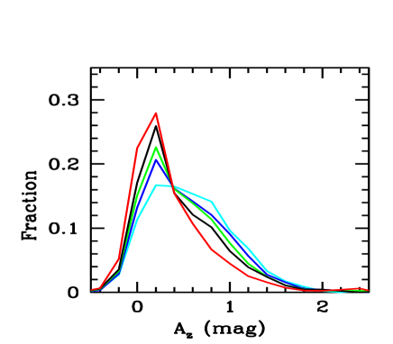
Figure 4: The fraction of the total stellar mass in the Universe contained in galaxies as a function of A_z, the z-band attenuation in magnitudes. The different colour lines represent different local densities as in Fig. 2.

5 Environmental Dependence of the Relations between the Physical Properties of Galaxies

In Kauffmann et al (2003b; hereafter Paper II), we studied the relations between the stellar masses, sizes, internal structure, and star formation histories of galaxies. We showed that strong correlations exist between these different properties. We also showed that the galaxy population as a whole divides into two distinct “families”. Below a characteristic stellar mass of $\sim 3\times 10^{10}M_{\odot}$, galaxies have low surface densities and concentrations typical of disk systems. They also have young stellar populations and a significant fraction have experienced recent starbursts. At stellar masses above $3\times 10^{10}M_{\odot}$, galaxies have high surface densities and concentrations typical of bulges. The majority have old stellar populations.

Because properties such as stellar age, mass and surface density are so strongly correlated, it is important to understand not only how a single property correlates with environment, but also how the relations between different properties change as a function of environment. This is the topic of the present section.

5.1 The Relations between Structural Parameters and Stellar Mass

In Paper II we studied how the surface mass density $\mu_{*}$ and concentration index $C$ of galaxies vary as a function of their stellar mass $M_{*}$. We found that surface mass density correlates tightly with stellar mass. Below a mass of $3\times 10^{10}M_{\odot}$, the median surface mass density scales with mass as $\mu_{*}\propto M_{*}^{0.63}$. At larger masses, the scaling of $\mu_{*}$ with $M_{*}$ becomes weaker and $\mu_{*}$ eventually saturates at at a value of around $10^{9}M_{*}$ kpc^-2. In Fig. 5 we plot the $\mu_{*}-M_{*}$ and $C-M_{*}$ relations for galaxies split into six density bins . The solid lines indicate the median value of $\log\mu_{*}$ or $C$ as a function of $\log M_{*}$, while the dotted lines indicate the 10th and 90th percentiles of the distributions. Note that we weight each galaxy by $1/V_{max}$ when we calculate these distributions, but we only plot the relations over the ranges in stellar mass where we have at least 200 galaxies per bin. We find that for galaxies with $M_{*}>3\times 10^{10}M_{\odot}$, the $\mu_{*}-M_{*}$ and $C-M_{*}$ relations are remarkably independent of density. Galaxies with masses smaller than $3\times 10^{10}M_{\odot}$ have slightly higher concentrations and surface densities in the very densest environments.

Recall that the surface mass density is proportional to the stellar mass divided by the square of the half-light radius of the galaxy in the $z$-band. The invariance of the $\mu_{*}-M_{*}$ relation for massive galaxies thus implies that the size distribution of these galaxies does not depend on environment. The concentration index has frequently been used a proxy for Hubble type. It was shown by Shimasaku et al (2001) and Strateva et al (2001) that for bright galaxies there is a good correspondence between $C$ index and ‘by-eye’ classification into Hubble type, with $C\sim 2.6$ marking the boundary between ‘early-type’ galaxies (elliptical, S0s and Sas) and ‘late-type’ galaxies (Sb-Irr). Conventional widom states that galaxy morphology correlates with local density (Dressler 1980), so at first glance it is astonishing to find no significant variation in the $C-M_{*}$ relation as a function of environment.

The most likely solution to this paradox is that ‘by-eye’ classification into Hubble type is dependent not only on the structure of the galaxy, but also on its star formation rate. This was noted by Koopmann & Kenney (1998) who showed that in the Virgo cluster, spirals with reduced global star formation activity are often assigned early-type classifications irrespective of their central light concentrations. As we will show in the next section, the relations between star formation rate and the structural parameters of galaxies do vary strongly with environment for galaxies of all stellar masses.

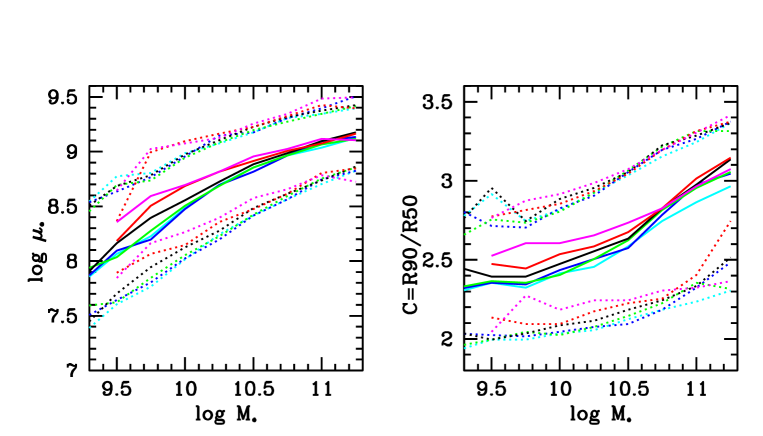
Figure 5: The relations between surface mass density and stellar mass (left) and concentration index and stellar mass (right) are plotted for galaxies in six different density bins as follows: cyan, 0 or 1 neighbour; blue, 2-3 neighbours; green, 4-6 neighbours; black, 7-11 neighbours; red, 12-16 neighbours; magenta, 17 or more neighbours. The solid curves indicate the median value of $\log\mu_{*}$ or $C$ and a given value of $\log M_{*}$. The dotted lines indicate the 10th and 90th percentiles of the distributions.

5.2 The Relations between Star Formation History, Stellar Mass and Galaxy Structure

Figure 6: A scatterplot of $g-r$ colour versus stellar mass is plotted for 1000 galaxies in our lowest density bin (N_neighb=0-1; left) and our highest density bin (N${}_{neighb}>17$; right).

In Paper II, we presented the conditional density distributions of two stellar age indicators, the 4000 Å break strength D_n(4000) and the H$\delta_{A}$ index as functions of stellar mass, stellar surface density and concentration. Brinchmann et al (2003) presented the distribution of the normalized star formation rate (SFR/$M_{*}$) as functions of these same parameters. Baldry et al (2003) studied the distribution of galaxy colours as a function of their absolute magnitudes. All these studies reach very similar conclusions. Faint low mass galaxies with low concentrations and surface mass densities have young stellar populations, ongoing star formation and blue colours. Bright galaxies with high stellar masses, high concentrations and high surface densities have old stellar populations, little ongoing star formation and red colours. A transition from “young” to “old” takes place at a characteristic stellar mass of $3\times 10^{10}M_{\odot}$, a stellar surface density of $3\times 10^{8}M_{*}$kpc^-2, a concentration index of 2.6 and an r-band absolute magnitude of $\sim-20.3$. So how do the relations between stellar age, stellar mass and structural parameters depend on environment?

In Fig. 6, we show scatterplots of $g-r$ colour versus stellar mass for a random sample of 1000 galaxies in our lowest density and highest density bins. This plot clearly illustrates the “bimodal” colour-magnitude distribution of galaxies described in Baldry et al (2003); galaxies separate rather cleanly into a red sequence and a blue sequence. As density increases, we find that the relative weight of the two populations shifts from the blue to the red sequence. In the highest density environments, the red sequence dominates entirely. This is well-known from studies of galaxy populations in nearby clusters.

In the top two panels of Fig. 7 we show how the median values of D_n(4000) and SFR/$M_{*}$ vary as a function of stellar mass for our different density bins. (Note that in Fig.7 we have applied the appropriate volume-corrections to our sample.) The median values of both parameters shift systematically as density increases. The shift is largest for galaxies with stellar masses just below our characteristic mass of $3\times 10^{10}M_{\odot}$ and corresponds to more than a factor of 10 decrease in star formation rate from our lowest density to our highest density bins. At very high stellar masses ($>10^{11}M_{\odot}$), there is little change in the median SFR with density. Likewise for $M_{*}<10^{10}M_{\odot}$, the effect again becomes somewhat weaker.

The bottom two panels show how the D_n(4000)-C and D_n(4000)-$\mu_{*}$ relations change as a function of density. In the highest density regions, galaxies with low concentrations characteristic of disk-dominated systems ($C<2.6$) have considerably older stellar populations than galaxies of similar concentrations in low-density regions. Van den Bergh (1976) was the first to remark on a class of “anaemic spirals”, which occur most often in rich clusters and these systems have recently been studied in considerable detail using SDSS data by Goto et al (2003b). In Paper II, we demonstrated that stellar age indicators were more closely correlated with $\mu_{*}$ than with $M_{*}$. This conclusion is borne out once again in Fig. 7. The relation between D_n(4000) and $\mu_{*}$ appears less sensitive to environment than the relations between D_n(4000) and $M_{*}$ or $C$.

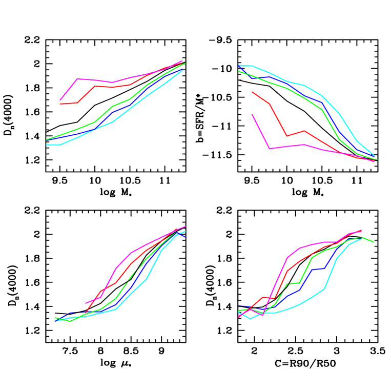
Figure 7: Top: The median relations between D_n(4000) and SFR/$M_{*}$ are plotted as a function of stellar mass for 5 different bins in density, colour-coded as in Fig. 5. Bottom: The median relations between D_n(4000) and $\mu_{*}$ (left) and $C$ (right).

5.3 Relations between Different Indicators of Star Formation History

So far we have used the 4000 Å break, the H$\delta_{A}$ absorption line index and the normalized star formation rate (SFR/$M_{*}$) interchangeably as indicators of the recent star formation history of a galaxy. In practice, these three indicators probe star formation on rather different timescales:

1. The normalized star formation rate is estimated using the fluxes of the nebular emission lines in the galaxy, in particular the H$\alpha$ line (Brinchmann et al 2003). SFR/$M_{*}$ thus probes star formation on a timescale equal to the lifetime of a typical HII region ($\sim 10^{7}$ years).

2. The strength H$\delta_{A}$ absorption line peaks once hot O and B stars have terminated their evolution and the optical light is dominated by late-B to early F-stars. This occurs about $3\times 10^{8}$ years after an episode of star formation.

3. The strength of the 4000 Å break increases montotonically with time. At stellar ages of more than $\sim 1$ Gyr, metallicity effects also become important.

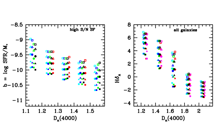
Figure 8: Top: The relations between SFR/$M_{*}$ and D_n(4000) (left) and H$\delta_{A}$ and D_n(4000) in different density bins colour-coded as in Figure 5. Solid circles indicate the median of the distribution, solid and open triangles are 25th and 75th percentiles, solid and open squares are 10th and 90th percentiles.

Insight into the nature of the recent star formation histories of galaxies may be obtained by studying correlations between these different indicators. In Paper II we showed that at a given value of D_n(4000), low mass galaxies span a significantly larger range in H$\delta_{A}$ equivalent width than high mass galaxies. This indicates that the recent star formation histories of low mass galaxies have been more bursty. This conclusion was confirmed by Brinchmann et al (2003), who showed that the distribution of SFR/$M_{*}$ for low mass galaxies exhibited a significant tail to high values. This tail was largely absent for high mass galaxies.

In this section, we investigate whether environment has any detectable influence on the recent star formation histories of the galaxies in our sample. Recent bursts of star formation would produce a tail of galaxies with large H$\delta_{A}$ equivalent widths and large values of SFR/$M_{*}$ at moderate values of D_n(4000). A recent sudden truncation in star formation (caused by ram-pressure stripping, for instance) would produce a population of galaxies with relatively low 4000 Å break strengths and high H$\delta$ equivalent widths, but with no detectable emission lines.

In Fig. 8, we plot the relation between SFR/$M_{*}$ and D_n(4000) and the relation between H$\delta_{A}$ and D_n(4000) for galaxies in our different density bins. The different symbols indicate different percentiles of the distribution: solid and open squares the 10th and 90th percentiles, solid and open triangles the 25th and 75th percentiles, and solid circles the median. As before, different colours indicate our different bins in density. Note that we only show the correlation between SFR/$M_{*}$ and D_n(4000) for galaxies with $S/N>3$ in the four emission lines H$\alpha$, H$\beta$, [OIII] and [NII]. For this subset of galaxies, it is possible to estimate the star formation rate in a reliable way using only the emission lines (see Brinchmann et al 2003). Because strong emission-line galaxies become increasingly rare in high density regions and in galaxies with old stellar populations, it is not possible to extend the analysis to the full sample. The correlation between H$\delta_{A}$ and D_n(4000), on the other hand, can be plotted for all the galaxies in the sample.

As can be seen, the relations between the different indicators show no dependence on environment. We have also restricted the analysis to galaxies with stellar masses in the range $3\times 10^{9}-3\times 10^{10}M_{\odot}$ and we find the same result. In section 5.2 we demonstrated that galaxies are systematically younger in low density regions and older in high density regions. Nonetheless, the results in this section indicate that the blue galaxies that do exist in high density regions appear to have recent star formation histories that are indistinguishable from those in the ‘field’. This suggests that the decrease in star formation activity in galaxies in high density regions occurs over relatively long ($>$ 1 Gyr) timescales for the majority of galaxies. We will come back to this point in section 7.

5.4 Other Properties associated with Star Formation: AGN and Dust

5.4.1 Nuclear activity in galaxies

In Kauffmann et al (2003c), it was demonstrated that Type 2 (narrow-line) active galactic nuclei occur almost exclusively in galaxies with stellar masses greater than $10^{10}M_{\odot}$. Weak AGN (those with [OIII] line luminosities less than $10^{7}$ L_⊙) occur in massive galaxies with predominantly old stellar populations, whereas powerful AGN (L[OIII]$>10^{7}$ L_⊙ ) are found in massive galaxies containing young stars. Because star formation is so strongly correlated with environment, it would be natural to expect that the incidence of powerful AGN would also be a function of local density.

Kauffmann et al (2003c) also showed that at luminosities below $10^{7}L_{\odot}$, the fraction of detected AGN in SDSS galaxies is a strong function of redshift. At larger distances, more of the host galaxy light falls within the fibre aperture and weak AGN become progressively more difficult to detect. At luminosities above $10^{7}L_{\odot}$, there were no longer any distance-dependent selection effects in picking out AGN using diagnostic diagrams based on emission line ratios. In the left panel of Fig.9, we plot the fraction of galaxies containing strong AGN with L[OIII]$>10^{7}L_{\odot}$ as a function of stellar mass in three bins of density. As expected, the fraction of strong AGN in massive galaxies decreases as a function of density. Kauffmann et al showed that the fraction of powerful AGN in galaxies with $3\times 10^{10}-10^{11}M_{\odot}$ was $\sim 0.1$ for the galaxy population as a whole. In our lowest density bin, the fraction rises to $\sim 0.15$ and in our highest density bin, it is $\sim 0.06$.

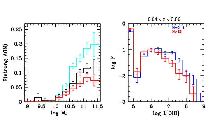
Figure 9: Left: The fraction of galaxies containing AGN with L[OIII]$>10^{7}$ $L_{\odot}$ is plotted as a function of stellar mass for three bins in density. Cyan is for galaxies with $N_{neighb}=0-1$, black is for $N_{neighb}=7-11$ and red is for $N_{neighb}>12$. Right: The distribution of [OIII] luminosities of AGN in galaxies with stellar masses in the range $3\times 10^{10}-3\times 10^{11}M_{\odot}$ in high density environments (red) and in low density environments (blue). The sample has been restricted to galaxies with $0.04<z<0.06$. Note that the [OIII] luminosities have been corrected for dust attenuation as described in Kauffmann et al (2003c).

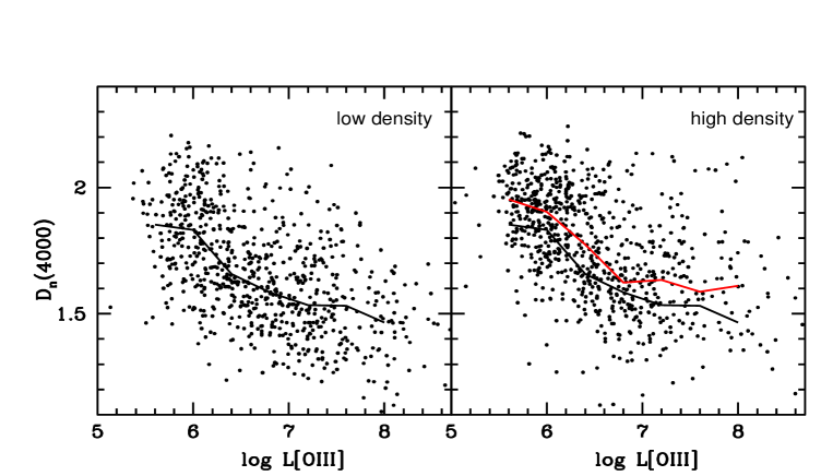
Figure 10: D_n(4000) is plotted as a function of L[OIII] for AGN with $0.08<z<0.1$ in low density regions (left) and in high-density regions(right). The black line shows the running median of the distribution of points in low-density regions and the red line is the same for the high-density points.

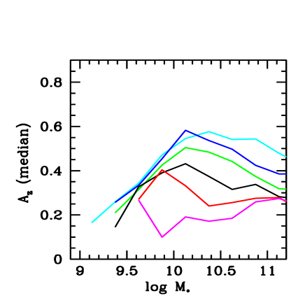
Figure 11: The median $z$-band attenuation due to dust in magnitudes is plotted as a function of stellar mass in the same density bins as in Fig. 5

Figure 12: Dust attenuation in the $z$-band is plotted against D_n(4000) for galaxies with $11<\log M_{*}<11.5$ in low-density regions (left) and in high-density regions (right).

Miller et al (2003) have also used SDSS data to study how the fraction of galaxies with AGN varies as a function of environment. They found almost no density dependence and concluded that AGN were unbiased tracers of large-scale structure in the Universe. Miller et al did not classify their AGN according to [OIII] luminosity, and it is likely that their sample included a substantial number of weak AGN. In the right panel of Fig. 9, we plot the distribution of [OIII] luminosities of AGN in galaxies with stellar masses in the range $3\times 10^{10}-3\times 10^{11}M_{\odot}$ and in two different bins of density. In order to avoid distance-dependent selection effects, we have restricted the analysis to galaxies with $0.04<z<0.06$. Note that all galaxies without any detectable AGN are placed into the first bin. As can be seen, it is the fraction of powerful AGN with L[OIII]$>10^{7}L_{\odot}$ that depends on density. As discussed in Kauffmann et al (2003c), AGN with these luminosities are almost all type 2 Seyfert galaxies. On the other hand, the fraction of low-luminosity AGN (LINERs) depends very little on local density. Since there are many more LINERs than Seyferts, the overall fraction of detected AGN shows little environmental dependence.

It is interesting to ask whether the physical mechanism responsible for the decrease in powerful AGN fraction in high density regions is the same as that responsible for the decrease in the fraction of star-forming galaxies. If this is the case, then the relation between [OIII] luminosity and 4000 Å break strength in AGN should not depend on environment. In Fig. 10, we show the relation between D_n(4000) and L[OIII] for AGN in low-density ($N_{neighb}<2$) and high density ($N_{neighb}>12$) environments. We find little change in the D_n(4000)-L[OIII] relation with density. There is a slight shift towards higher D_n(4000) at given L[OIII] in denser regions. We have also investigated whether there is any environmental dependence of the stellar masses or structural parameters of the host galaxies of AGN of given L[OIII]. All these studies indicate that at given [OIII] line luminosity, the properties of an AGN host depend very little on local density. It is the overall fraction of galaxies that are able to host strong-lined AGN that decreases in high-density environments.

5.4.2 Dust

Dust attenuation is another property that can be expected to be strongly correlated with how much ongoing star formation is taking place in a galaxy. In Fig. 4 we showed that in low-density regions of the Universe, a larger fraction of the total stellar mass is in galaxies with significant dust attenuation. In Fig. 11, we plot the relation between the median value of the dust-attenuation in the $z$-band and stellar mass for galaxies in different bins in density. As can be seen, for galaxies with $M_{*}>10^{10}M_{\odot}$, the amount of dust in a galaxy of given mass is a relatively strong function of density. For low mass galaxies, the amount of dust shows little dependence on environment. It is interesting that in low-density environments, even very massive galaxies contain a substantial amount of dust. Once again it is interesting to ask whether this is simply a consequence of the fact that there is more star formation in massive galaxies in low-density environments.

In Fig. 12 we plot the relation between the 4000 Å break and dust attenuation for massive galaxies with $10^{11}M_{\odot}<M_{*}<3\times 10^{11}M_{\odot}$ in our lowest density bin (left) and in our highest density bin (right). As can be seen, the dust attenuation is tightly correlated with D_n(4000). In low density regions, a substantial fraction of high mass galaxies have low 4000 Å break strengths and high attenuation. In high density regions, almost all massive galaxies have both large break strengths and low attenuation. However, the correlation between A_z and D_n(4000) is very similar in all environments. This indicates that the same mechanism is likely responsible for the decrease both in star formation and in dust content for galaxies in high density regions of the Universe.

6 The Scale Dependence of the Environmental Effect

In the previous two sections, we demonstrated that quantities associated with star formation history – colour, 4000 Å break, SFR/$M_{*}$ – show strong correlations with local density. In this section we ask whether we can place any constraints on the physical scale over which this correlation occurs. As discussed in section 3, theoretical considerations lead one to expect that galaxy properties should correlate best with dark matter density on small ($\sim$ 1 h^-1 Mpc) scales. There have been some recent suggestions in the literature, however, that star formation shows strong sensitivity to the density of galaxies evaluated on scales in excess of 5 Mpc (Balogh et al 2003).

In order to address this issue, we restrict the analysis in this section to galaxies in the redshift range $0.04<z<0.06$. This reduces the total number of galaxies in our sample by a large factor, but it has the advantage that at low redshifts, the galaxy population in the SDSS is densely sampled. It is then possible to explore the effect of an increase or a decrease in the size of the volume inside which we evaluate the counts.

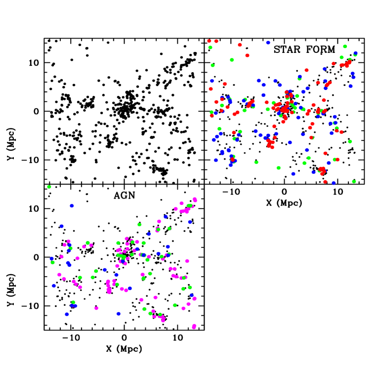
Figure 13: Top Left: The distribution of all galaxies in a ‘slice’ at z=0.05 (see text for more details). Top Right: Galaxies with $10^{10}M_{\odot}<M_{*}<3\times 10^{10}M_{\odot}$ are colour-coded according their measured 4000 Å break strengths. Red is for D_n(4000)$>1.8$, green is for $1.6<$ D_n(4000)$<1.8$ and blue is for D_n(4000)$<1.6$. (Note that galaxies falling out of the mass range are shown as smaller black dots) Bottom: Galaxies hosting AGN are colour-coded according to L[OIII]. Magenta is for log L[OIII]$<6.5$, green is for $6.5<$log L[OIII] $<7$, and blue is for log L[OIII]$>7$. Galaxies with no AGN is shown as small black dots.

To begin, Fig. 13 illustrates how galaxies with different star formation histories populate a typical large scale structure at z=0.05. We searched the group and cluster catalogue of Miller et al (2004, in preparation) for collections of galaxy groups with very similar redshifts spread over a field of less than 10 square degrees. We found several such associations and Fig. 13 shows an example of a rich system of galaxy groups at z=0.05. We have placed the origin of our x-and y–axes at the centre of the largest group in the field, which has a velocity dispersion of $\sim 500$ km s^-1. We plot a ‘slice’ that includes all galaxies with $cz$ within 500 km s^-1 of the brightest galaxy in the group. The structures shown in Fig. 13 occupy a relatively thin sheet that is aligned perpendicular to the line-of-sight. As can be seen, the densest structures in the sheet appear to be arranged along filaments that extend over scales of several tens of Mpc.

The top left panel in Fig. 13 shows the distribution of all the galaxies in the slice with spectroscopic redshifts. In the top right panel we have colour-coded galaxies with $10^{10}M_{\odot}<M_{*}<3\times 10^{10}M_{\odot}$ according to their measured 4000 Å break strengths. Red indicates galaxies with D_n(4000)$>1.8$, green is for galaxies with $1.6<$ D_n(4000)$<1.8$, and blue is for galaxies with D_n(4000)$<1.6$. As shown in Paper II, field galaxies with $M_{*}<3\times 10^{10}M_{\odot}$ generally have D_n(4000) $<1.6$. One should thus be able to evaluate the scale over which star formation responds to local density simply by looking at the distribution of the red and green points in the diagram. As can be seen, clumps of red galaxies appear wherever there is a significant overdensity in the distribution of galaxies, even when the overdensity only exists on small ($<1-2$ Mpc) scales. In the bottom panel we have coloured-coded galaxies with detected AGN according to their measured [OIII] line luminosities. The qualitative picture is very similar. AGN with high values of L[OIII] are found predominantly in low-density regions, while low-luminosity AGN are also found in denser groups.

Fig. 14 places our result on more quantitative footing. We take all the galaxies in our sample with $0.04<z<0.06$ and calculate counts within a nested series of shells in projected radius. We keep the allowed velocity difference fixed at 500 km s^-1. Note that tracer galaxies are now defined as galaxies with $r<17.77$ at z=0.06, so target galaxies will have more neighbours in this analysis. The top right panel of Fig. 14 shows how the 4000 Å break strength of galaxies with $10^{10}M_{\odot}<M_{*}<3\times 10^{10}M_{\odot}$ correlates with $N_{neighb}$ calculated within a projected radius of 1 Mpc. We have ordered all the galaxies in increasing order of $N_{neighb}$ and we then divide them into groups of 150. We plot the median value of D_n(4000) in each group as a function of the median value of N_neighb in that group. As can be seen, there is a very tight correlation between D_n(4000) and galaxy count on scales less than 1 Mpc. In the top right panel of Fig. 14, we plot the same thing, except that $N_{neighb}$ is evaluated within a radius of 5 Mpc. As can be seen, D_n(4000) does correlate with N_neighb even on these large scales, but the correlation is significantly weaker and noisier.

We can also ask whether the density on large scales has any influence on the star formation history of a galaxy, once the density on small scales is specified. The answer to this is shown in the two bottom panels of Fig. 14 where we plot D_n(4000) as a function of the number of neighbours with $1<R_{proj}<3$ Mpc, for galaxies with 0-1 neighbours inside 1 Mpc (bottom left) and for galaxies with 8-12 neighbours inside 1 Mpc (bottom right). As can be seen, the count within the 1-3 Mpc shell has no influence on D_n(4000). Finally, we have divided our galaxy sample into ten different bins in density using $R_{proj}<1$ Mpc and we calculate the linear correlation coefficient $r$ between D_n(4000) and the galaxy count in the shell with $1<R_{proj}<3$ Mpc. We find values of $r$ that scatter around zero and the distribution is entirely consistent with the null hypothesis of no correlation. We note that Balogh et al (2003) carried out a similar analysis and obtained the opposite result. We do not currently understand the reason for this.

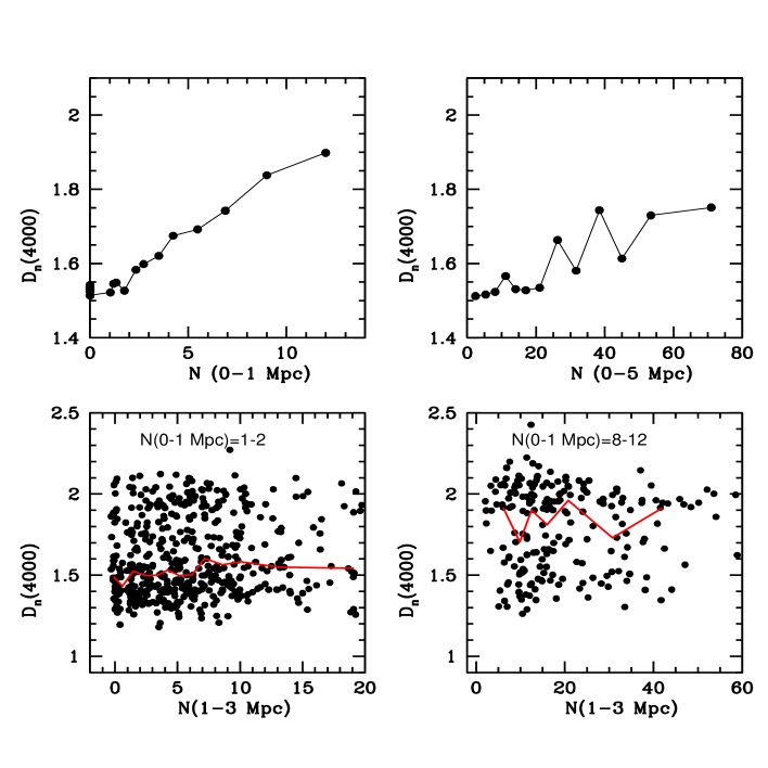
Figure 14: Top: The correlation between D_n(4000) and the number of neighbours within a projected radius of 1 Mpc (left) and 5 Mpc (right). The solid circles indicate the median value of D_n(4000) at given value of the count. We have chosen our bins so that they always include a fixed number of galaxies (150). Bottom: D$n$(4000) is plotted as a function of the count within the shell with $1<R_{proj}<3$ Mpc for galaxies with a fixed value of the count within 1 Mpc. The red line is a running median, evaluated such that fixed number of galaxies are included in every bin.

7 Summary and Discussion

7.1 Summary of the Main Observational Results

1. The characteristic stellar mass of galaxies increases as a function of density.

2. For stellar masses above $3\times 10^{10}M_{\odot}$, the distribution of size and concentration at fixed stellar mass is independent of local density. Galaxies with $M_{*}<10^{10}M_{\odot}$ tend to be slightly more concentrated and more compact in the densest regions.

3. The galaxy property that is most sensitive to environment is star formation history. The relations between D_n(4000) or SFR/$M_{*}$ and galaxy mass depend strongly on density. The dependence is strongest for galaxies with stellar masses less than $3\times 10^{10}M_{\odot}$. For these systems, the median SFR/$M_{*}$ changes by more than a factor of 10 from our lowest density to our highest density bin. The dependence is weaker for high mass galaxies, but it remains significant.

4. The correlation between star formation history and local density is strongest on small ( 1 Mpc) scales. We see no evidence that the density on large scales has any influence on the star formation history of a galaxy once the density on small scales is specified.

5. The relations between our three different indicators of recent star formation history – the 4000 Å break strength D_n(4000), the Balmer-absorption index H$\delta_{A}$, and the normalized star formation rate SFR/$M_{*}$– do not depend on environment.

6. A larger fraction of galaxies host AGN with high [OIII] line luminosities in low density environments. At a given value of L[OIII], the properties of AGN hosts do not appear to depend on environment.

7. Galaxies in low-density environments contain more dust. This is true even for the most massive galaxies in our sample with $M_{*}>10^{11}M_{\odot}$.

7.2 From Local Density to Halo Mass

In order to interpret our results, it is critical to understand how physical conditions change as a function of the particular local density estimates that we have used in our analysis.

As discussed in section 3, one advantage of characterizing the environment of a galaxy in terms of its membership in a group or cluster, is that it is possible to assign each object to a dark matter halo of a well-defined mass. Inside such a halo, galaxies move with a known distribution of velocities and the thermodynamic state of the intergalactic gas is also reasonably well-constrained. The link between our local galaxy density estimate and halo mass is not as straightforward, but considerable insight may be gained by analyzing mock galaxy catalogues generated using cosmological N-body simulations.

In this section, we make use of the publically available dark matter halo and galaxy catalogues from the GIF simulations described in
Kauffmann et al (1999; http://www.mpa-garching.mpg.de/galform/virgo/hrs/) to illustrate how this may be achieved in practice. These simulations are for standard $\Lambda$CDM initial conditions ($\Omega=0.3$, $\Lambda=0.7$, $h=0.7$, $\sigma_{8}=0.9$) and were carried out in a periodic box of length 141 $h^{-1}$ Mpc. The mass of individual dark matter particles in the simulation is $1.4\times 10^{10}h^{-1}M_{\odot}$. As explained in Kauffmann et al, the history of a galaxy that forms inside a dark matter halo containing more than 100 particles can be tracked reasonably reliably in these simulations. The GIF catalogues are thus limited to galaxies with stellar masses larger than $2\times 10^{10}M_{\odot}$ or $r$-band magnitudes brighter than $\sim-20.5$. This corresponds rather well to the magnitude limit of our volume-limited sample of SDSS tracer galaxies.

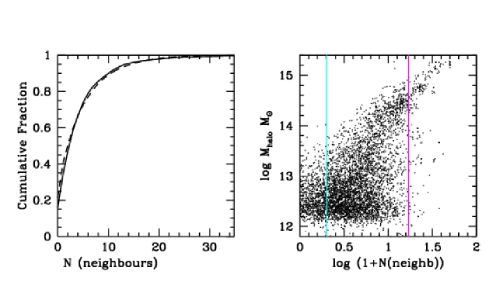
Figure 15: Left: The cumulative fraction of galaxies with counts less than $N$ for the simulated galaxies (solid) and for the observed galaxies (dashed). Right: The virial mass of the halo in which a galaxy resides is plotted as a function of the logarithm of the counts around the galaxy. A random number in the range 0-0.5 has been added to each count in order to obtain a uniform distribution in the abscissa. The vertical cyan and magenta lines indicate the locations of our two extreme bins in local density.

We have placed a cylinder of radius 2 Mpc and length 14.3 Mpc around each galaxy in the catalog and we count the total number of galaxies contained inside each cylinder. The left-hand panel of Fig. 15 compares the distribution of counts around our simulated galaxies (solid line) with the distribution of counts around the observed galaxies shown in Fig. 1. As can be seen, the two distributions agree well. In the right-hand panel we show a scatter-plot of the mass of the dark matter halo in which the simulated galaxy resides as a function of the count within the cylinder. This shows that galaxies with less than two neighbours reside in halos with virial masses between $10^{12}$ and $10^{13}M_{\odot}$. Note that these galaxies occupy the density bin represented by cyan lines in the figures shown in section 6. In this bin, one is thus studying a population of objects where there is typically only one bright galaxy per halo. Galaxies with more than 17 neighbours (represented by magenta lines in section 6) nearly always reside in halos more massive than $10^{14}M_{\odot}$, i.e. in galaxy clusters. Galaxies in our intermediate density bins occupy halos with a rather wide range in mass. However, the median halo mass increases as a a function of the number of neighbours, which explains why galaxy properties change continuously as a function of our local density estimates.

We note that the above analysis is only meant to be illustrative. We have not yet studied whether our simulated galaxies match the observations in detail. In addition, the GIF simulations lack the resolution to study galaxies with stellar masses below $\sim 10^{10}M_{\odot}$. However, the trend for galaxies with higher local density estimates to occupy more massive halos should be robust.

7.3 From Dark Matter Halos to Galaxies

Once we make a link between the estimate of the density around a galaxy and the characteristic mass of the halo in which it resides, the observed trends place important constraints on galaxy formation processes.

For example, Fig. 3 shows that most of the change in the characteristic stellar masses of galaxies occurs in our low-density (cyan and blue) bins. The partition function of the stellar mass remains almost invariant in our higher-density (green, black and red) bins. If we now make the identification with halo mass shown in Fig. 15, we infer that the stellar mass of galaxies increases with halo mass for halos with virial masses less than a few $\times 10^{13}M_{\odot}$. In more massive halos, the distribution of stellar masses no longer depends on $M_{halo}$. One way to explain this trend is if galaxies no longer form stars once they fall into high mass halos. This is qualitatively supported by the data, which show that in general, the star formation rates of galaxies decrease strongly in high density environments. However, the nature of this decrease is clearly quite complicated. Figs. 2 and 3 show that the fraction of the total stellar mass in star-forming galaxies decreases continuously with density. In Fig. 7 one sees that for low mass galaxies ($\sim 10^{10}M_{\odot}$) the drop in SFR/$M_{*}$ occurs primarily in very high density environments that contain massive halos. For high mass galaxies ($\sim 10^{11}M_{\odot}$) the overall drop in SFR/$M_{*}$ with density is much smaller and it takes place mainly in our lowest density bins.

There are many different physical processes that could, in principle, play a role in quenching star formation in massive halos. Gunn & Gott (1972) discussed how the interstellar material in a galaxy would feel the ram pressure of the intracluster medium as it moves through the cluster. They calculated that for a galaxy moving at the typical velocity of 1700 km/s through the Coma Cluster, the ISM would be stripped in one pass. Farouki & Shapiro (1981) used N-body simulations to show that tidal interactions between galaxies in clusters are effective in destroying galactic disks, a process dubbed “harrassment” by Moore et al (1996). In semi-analytic models of galaxy formation, star formation in disk galaxies is maintained by cooling and infall from a surrounding halo of hot gas. When a galaxy falls into a large halo, this diffuse halo is stripped and star formation in the galaxy gradually declines as it uses up its cold gas (e.g. Kauffmann, White & Guiderdoni 1993; Diaferio et al 2001) Such a gas supply-driven decline in the star formation rates of cluster galaxies was first suggested by Larson, Tinsley & Caldwell (1980) and in some recent papers it has also been called strangulation (e.g. Balogh & Morris 2000; Balogh, Navarro & Morris 2000). Other ICM-driven processes that have been discussed in the literature include evaporation (Cowie & Songaila 1977) and turbulent viscous stripping (Nulsen 1982).

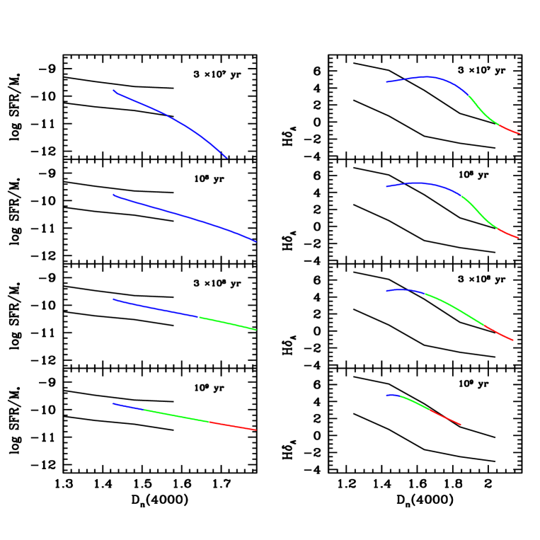
Figure 16: The evolution of a galaxy that has been forming stars at a continuous rate for 10 Gyr following trucation in its star formation rate. Results are shown for different quenching timescales, as defined in the text. The blue part of curve shows the evolution for the first 0.5 Gyr following the quenching of the star formation, green is for t=0.5-1.5 Gyr and red is for t=1.5-2.5 Gyr. The black lines delineate the 10 and 90 percentiles of the observed relations shown in Fig. 8.

We note that for massive galaxies, harrassment is not favoured by the observations, because it is difficult to explain why the sizes and concentrations of galaxies of fixed mass do not depend on environment, if disks are destroyed in high density regions. Another way to distinguish between these different processes is through constraints on the timescale over which the star formation is quenched in high mass halos. If ram-pressure stripping of the interstellar medium is the most important process, then this timescale is expected to be short ($\sim 10^{7}$ years). If instead gas-supply driven processes are the dominant factor, then the decline should be more gradual.

The facts that star-forming galaxies are currently present in low-density environments and that the fraction of such objects declines continuously with increasing density, imply that quenching processes are still operating. In Fig. 8, we demonstrated that the relations between three different indicators of recent star formation history – the 4000 Å break strength, the Balmer-absorption index H$\delta_{A}$ and the normalized star formation rate SFR/$M_{*}$– do not depend on environment. This means that when star formation in a galaxy is quenched, its values of D_n(4000), H$\delta_{A}$ and SFR/$M_{*}$ must change in such a way that the galaxy evolves along these relations. In Fig. 16 we demonstrate that this requires star formation to decline on relatively long ($>1$ Gyr) timescales.

Let us consider a galaxy that has been forming stars at a continuous rate (SF₀) for 10 Gyr (i.e $\log\rm{SFR/M}_{*}\sim-10$). As shown by Brinchmann et al (2003), the distribution of SFR/$M_{*}$ for star-forming galaxies peaks at values close to this over nearly 3 orders of magnitude in stellar mass, declining only at $M_{*}>$ few $\times 10^{1}0M_{\odot}$. According to the population synthesis models of Bruzual & Charlot (2003), such a galaxy is predicted to have D_n(4000)$\sim 1.4$ and H$\delta_{A}\sim 4$. After 10 Gyr of continuous star formation, we let the star formation rate evolve as SFR(t)= SF₀ $\exp(-t/\tau_{q})$, where $\tau_{q}$ is the characteristic timescale over which the star formation is quenched in the galaxy. Fig. 16 shows how the galaxy moves in the SFR/M_∗-D_n(4000) and H$\delta_{A}$-D_n(4000) planes for different values of $\tau_{q}$ The blue part of the curve shows the evolution for the first 0.5 Gyr after the star formation rate begins to decline. The green part of the curve is for t=0.5-1.5 Gyr and red is for t=1.5-2.5 Gyr. As can be seen, galaxies move along the relations defined by observed galaxies only if the quenching timescale is long ($\tau_{q}>$ 1 Gyr). If the quenching timescale is short, the galaxy will move away from the main body of the data and stay there for a period of up to 1.5 Gyr. The H$\delta_{A}$-D_n(4000) relation turns out to be more constraining than SFR/M_∗-D_n(4000), because it is defined for all the galaxies in the sample, not just for those with emission lines and young stellar ages.

Although we have argued star formation in the majority of galaxies is being quenched over long timescales, clear exceptions do exist.   Quintero et al (2003) have identified a population of “K+A” galaxies in the SDSS with spectra exhibiting strong Balmer absorption lines, but with little or no H$\alpha$ emission. However, such galaxies are currently very rare ($<$1% of the total population). Balogh et al (2003) have argued that the timescale for quenching processes ought to be short, citing the fact that the distributions of H$\alpha$ equivalent widths of star forming galaxies are independent of environment. Our arguments contradict this. Fig. 16 shows that for slow quenching galaxies should move along the observed relations, while rapid quenching would lead to an overabundance of “K+As”. More detailed modelling is clearly necessary in order to settle this question. An estimate of the recent accretion rate of galaxies onto massive halos is required in order to set tight limits on quenching timescales. In addition, it is necessary to adopt a range of different star formation histories in order to account for the observed scatter of our ‘blue’ galaxies in the H$\delta_{A}$-D_n(4000) plane. We will leave more detailed analysis of this kind for a future paper.

7.4 From Low Density to High Redshift

In section 7.1, we showed that there is a correspondence between our estimate of the local density around a galaxy and the mass of the dark matter halo in which it resides. In the now-standard $\Lambda$CDM cosmology, structure in the Universe builds up via a process of hierarchical clustering, with small structures merging together to form larger and larger objects. At high redshifts, the abundance of massive halos decreases and fewer galaxies reside in clusters and rich groups. This is illustrated in Fig. 17 where we show how the dark matter is partitioned among halos of different masses in our $\Lambda$CDM simulation at a series of different redshifts. The fraction of the matter that has collapsed and fallen into halos with masses less than $10^{13}M_{\odot}$ remains approximately constant from $z=0$ to $z=1$. However, the fraction of material in halos with masses greater than $10^{14}M_{\odot}$ decreases from 12 percent at $z=0$ to 1.5 percent at z=1. By redshift 2, the fraction of matter in halos between $10^{12}$ and $10^{13}M_{\odot}$ has also begun to decrease.

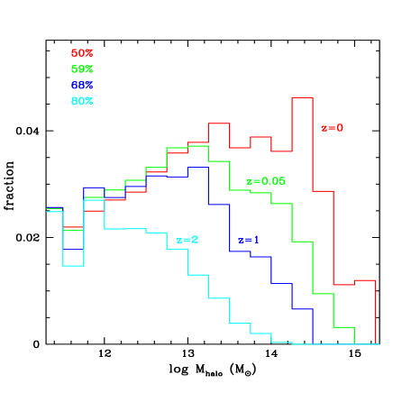
Figure 17: The fraction of the dark matter in the Universe in halos of different mass.

In one compares Fig. 17 with Fig. 15, one might naively speculate that ‘field’ galaxies at $z\sim 1$ would look much like galaxies in our low-density (cyan and blue) bins. Obviously the real situation is complicated by the fact that the Universe was only half its present age at $z=1$. Galaxies were therefore less ‘evolved’ than at the present day; they were probably more gas-rich and their stellar populations were younger and hence bluer and brighter. Nevertheless when one examines the trends in our data, a qualitiative analogy between galaxies in low-density environments and galaxies in the high-redshift Universe seems quite compelling.

The most striking evolutionary trend in the galaxy population from $z=0$ to $z\sim 1-2$ is the rapid increase in the global star formation rate density (Lilly et al 1996 ; Madau et al 1996). The reason for this evolution was first pointed out by Cowie et al (1996), who showed that the maximum rest-frame K-luminosity of galaxies that undergo rapid star formation has been declining smoothly with redshift from $z\sim 1$ to the present. Cowie et al. dubbed this process ‘down-sizing’ and this is exactly what is seen in Fig. 7. As local density increases, strong star formation occurs only in galaxies with progressively smaller and smaller stellar masses.

There has been considerable recent attention has focused on a population of extremely red objects (EROs) at $z>1$ (e.g. Elston et al 1988; Daddi, Cimatti & Renzini 2000; Cimatti et al 2002). These are massive galaxies with colours as red as (or in some cases even redder than) those of passively evolving elliptical galaxies. When studied spectroscopically, some of these galaxies turn out to be genuinely old systems, but a substantial fraction are forming stars and are red because they are very dusty. In fig. 12 we showed that as local density decreases, there are a larger fraction of very massive galaxies with star formation and strong dust attenuation.

Finally, it is interesting that quantities that are only weakly dependent on local density also seem to exhibit little change with redshift. Even though the inferred characteristic mass of dark matter halos decreases by a factor of $\sim 100$ from our highest density to our lowest density bins, Fig. 2 shows that the characteristic stellar masses of the galaxies in these halos decreases by only a factor of $\sim 2$. Studies of the evolution of the rest-frame near-IR luminosity function suggest that characteristic stellar masses of galaxies have evolved only weakly from $z\sim 1$ to the present (e.g. Pozzetti et al 2003; Somerville et al 2003). In Fig. 6, we showed that at given stellar mass, the sizes and concentrations of galaxies exhibit almost no dependence on environment. In a recent study of 168 galaxies with K-band magnitudes brighter than 23.5, Trujillo et al (2003) find that the relation between galaxy size and stellar mass has remained unchanged since $z\sim 3$. A study of the size-mass relation of several tens of thousands of galaxies in the GEMS/COMBO-17 survey leads to the same basic conclusion (MacIntosh et al, in preparation; Barden et al, in preparation).

7.5 Galaxy Formation: Nature or Nurture?

We began this paper by asking whether the correlations between the different physical properties of galaxies were imposed very early on (the “nature” hypothesis) or whether they are the end product of processes that have operated over a Hubble time (the “nurture” scenario). Our tentative, perhaps unsurprising conclusion, is that both nature and nurture are important for understanding the evolution of the galaxy population.

We have shown that the relations between between galaxy structural parameters and stellar mass exhibit little dependence on density. This suggests that these relations were in place relatively early on. As discussed above, studies of the distribution of galaxy sizes at high redshift also seem to support this conclusion.

We have also shown that the relation between star formation history and stellar mass is quite sensitive to local density. We note that most of the density-dependence is for galaxies with $M_{*}\sim 10^{10}M_{\odot}$. Very massive galaxies generally have old stellar populations, both in low density and in high density environments. Very low mass galaxies tend to have young stellar populations and exhibit only a weak drop in average star formation rate from our lowest density to our highest density bins.

Fig. 18 attempts to put these two findings together. In the top panels we plot D_n(4000) as a function of stellar mass for galaxies in our lowest density bin. Results are shown separately for disk-dominated galaxies with $C<2.6$ (left) and for bulge-dominated galaxies with $C>2.6$ (right). We only plot galaxies with $z<0.055$ so that our sample is volume-limited down to the lowest stellar masses shown on the plot. As can be seen, the division of the galaxy population into two distinct “families” (old, massive and concentrated; small, young and diffuse) persists even in our lowest density bin. In the bottom panel, we show the same for galaxies in our two highest density bins. We see that the “tail” of massive, star-forming early-type galaxies present in the low density bin has diminished and has been replaced by a uniform population of old “ellipticals”. At the same time, a significant number of disk-dominated galaxies with lower masses have stopped forming stars and have moved onto the red sequence.

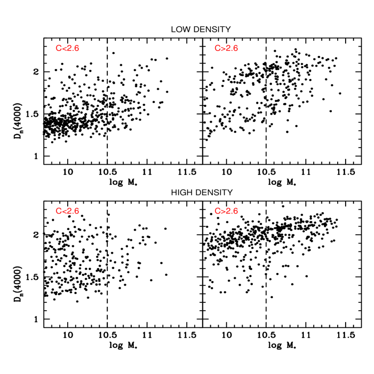
Figure 18: Top: D_n(4000) is plotted as a function of stellar mass for galaxies with $C<2.6$ (left) and $C>2.6$ in our lowest density bin (cyan in Fig. 2). Bottom: The same, except for galaxies in our two highest density bins (black and red in Fig. 2). We have plotted galaxies with $z<0.055$ so that the samples are volume-limited down to the lowest stellar masses shown in the plot.

Our results suggest that there are two basic routes by which galaxies reach the end-point of the evolution and become “dead and red”. The first is an event, for example a merger, that leads to the formation of a massive bulge and an associated black hole. During the event stars form very rapidly, the internal gas reservoir of the galaxy is depleted and subsequent cooling is strongly suppressed. The second route is the removal of the cold gas supply by external processes that operate in massive halos. This has very little effect on the structure of massive galaxies, which already have low gas fractions.

The majority of massive galaxies passed along the first route at relatively high redshifts and now have high concentrations and surface mass densities. Low mass galaxies, on the other hand, generally do not pass along this route and in low-density environments they are still actively forming stars. As low mass galaxies fall into massive halos, their cold gas supply is removed and their star formation shuts down. Massive galaxies are already near the end-point of their evolution when they fall into massive halos, but the same external process at work on the low-mass galaxies finishes the job. This not only shuts off any residual star formation in these systems, but also starves the black hole.

Considerable work remains to be done in understanding the physics that leads to the scaling relations presented in this paper. We believe that a combination of data from the new generation of large surveys, both at $z=0$ and at high redshifts, with insight gained from modern simulations of structure formation will be the key to unravelling how galaxies formed and evolved.

S.C. thanks the Alexander von Humboldt Foundation, the Federal Ministry of Education and Research, and the Programme for Investment in the Future (ZIP) of the German Government for their support. B.M. thanks the Florence Gould Foundation.

Funding for the creation and distribution of the SDSS Archive has been provided by the Alfred P. Sloan Foundation, the Participating Institutions, the National Aeronautics and Space Administration, the National Science Foundation, the U.S. Department of Energy, the Japanese Monbukagakusho, and the Max Planck Society. The SDSS Web site is http://www.sdss.org/.

The SDSS is managed by the Astrophysical Research Consortium (ARC) for the Participating Institutions. The Participating Institutions are The University of Chicago, Fermilab, the Institute for Advanced Study, the Japan Participation Group, The Johns Hopkins University, Los Alamos National Laboratory, the Max-Planck-Institute for Astronomy (MPIA), the Max-Planck-Institute for Astrophysics (MPA), New Mexico State University, University of Pittsburgh, Princeton University, the United States Naval Observatory, and the University of Washington.

References

Abazaijan, K. et al, 2003, AJ, 126, 2081

Baldry, I.K., Glazebrook, K., Brinkmann, J., Ivezic, Z., Lupton, R.H., Nichol, R.C., Szalay, A.S, ApJ, in press (astro-ph/0309710)

Balogh, M.L., Morris, S.L., 2000, MNRAS, 318, 703

Balogh, M.L., Navarro, J.F., Morris, S.L., 2000, ApJ, 540, 113

Balogh, M.L., Christlein, D., Zabludoff, A.I., Zaritsky, D., 2001, ApJ, 557, 117

Balogh, M.L. et al, 2003, submitted (astro-ph/0311379)

Benson, A.J., Cole, S., Frenk, C.S., Baugh, C.M., Lacey, C., 2000, MNRAS, 311, 793

Birnboim, D., Dekel, A., 2003, MNRAS, 345, 349

Blanton, M.R. et al, 2003a, ApJ, 594, 186

Blanton, M.R., Eisenstein, D.J., Hogg, D.W., Schlegel, D.J., Brinkmann, J, 2003b, ApJ, submitted (astro-ph/0310453)

Blanton, M.R. et al, 2003c, AJ, 125, 2348

Blanton, M.R., Lupton, R.H., Maley, F.M., Young, N., Zehavi, I., Loveday, J. 2003d, AJ, 125, 2276

Bower, R.G., 1991, MNRAS, 248, 332

Brinchmann, J., Charlot, S., White, S.D.M., Tremonti, C., Kauffmann, G., Heckman, T.M., Brinkmann, J., 2003, MNRAS, submitted (astro-ph/0311060)

Bruzual, G., Charlot, S., 2003, MNRAS, 344, 1000

Budavari, T., et al, 2003, ApJ, 595, 59

Charlot, S., Longhetti, M., 2001, MNRAS, 323, 887

Cimatti, A. et al, 2002, A&A, 381, L68

Daddi, E., Cimatti, A., Renzini, A., 2000, A&A, 362, L45

Davis, M., Geller, M.J., 1976, ApJ, 208, 13

Diaferio, A., Kauffmann, G., Balogh, M.L., White, S.D.M., Schade, D., Ellingson, E., 2001, MNRAS, 232, 999

Cowie, L.L., Songaila, A., 1977, Nature, 266, 501

Cowie, L.L., Songaila, A., Hu, E.M., Cohen, J.G., 1996, AJ, 112, 839

De Propris, R. et al, 2003, MNRAS, 342, 725

Diaferio, A., Kauffmann, G., Balogh, M.L., White, S.D.M., Schade, D., Ellingson, E., 2001, MNRAS, 328, 726

Dressler, A., 1980, ApJ, 236, 531

Elston, R., Rieke, G.H., Rieke, M.J., 1988, ApJ, 331, L77

Farouki, R., Shapiro, S.L., 1981, ApJ, 243, 32

Fukugita, M., Ichikawa, T., Gunn, J.E., Doi, M., Shimasaku, K., Schneider, D.P. 1996, AJ, 111, 1748

Gomez, P.L. et al, 2003, ApJ, 584, 210

Goto, T., Yamaguchi, C., Fujita, Y., Okamura, S., Sekiguchi, M., Smail, I., Bernardi, M., Gomez, P., 2003a, MNRAS, 346, 601

Goto, T. et al, 2003b, PASJ, 55, 757

Gunn, J., Carr, M., Rockosi, C., Sekiguchi, M., Berry, K., Elms, B., de Haas, E., Ivezić, Z. et al. 1998, ApJ, 116, 3040

Hashimoto,Y., Oemler, A., Lin, H., Tucker, D.L., 1998, ApJ, 499, 589

Hogg, D., Finkbeiner, D., Schlegel, D., & Gunn, J. 2001, AJ, 122, 2129

Hogg, D.W. et al, 2003a, ApJ, 585, L5

Hogg, D.W. et al, 2003b, ApJ, submitted (astro-ph/0307336)

Hoyle, F., Rojas, R.R., Vogeley, M.S., Brinkmann, J., ApJ, submitted (astro-ph/0309728)

Kauffmann, G., White, S.D.M., Guiderdoni, B., 1993, MNRAS, 264, 201

Kauffmann, G., Colberg, J.M., Diaferio, A., White, S.D.M., 1999, MNRAS, 303, 188

Kauffmann, G. et al, 2003a, MNRAS, 341, 33 (Paper I)

Kauffmann, G. et al, 2003b, MNRAS, 341, 54 (Paper II)

Kauffmann, G. et al 2003c, MNRAS, 346, 1055

Kodama, T., Smail, I., Nakata, F., Okamura, S., Bower, R.G., 2001, ApJ, 562, L9

Koopmann, R.A., Kenney, J.D.P., 1998, ApJ, 497, L75

Lacey, C., Cole, S., 1993, MNRAS, 262, 627

Larson, R.B., Tinsley, B.M., Caldwell, C.N., 1980, ApJ, 237, 692

Lemson, G., Kauffmann, G., 1999, MNRAS, 302, 111

Lewis, I., et al, 2003, MNRAS, 334, 673

Lilly, S.J., Le Fevre, O., Hammer, F., Crampton, D., 1996, ApJ, 460, L1

Madau, P., Ferguson, H.C., Dickinson, M.E., Giavalisco, M., Steidel, C.C., Fruchter, A., 1996, MNRAS, 283, 1388

Loveday, J., Maddox, S.J., Efstathiou, G., Peterson, B.A., 1995, ApJ, 442, 457

Madgwick, D.S. et al, 2003, MNRAS, 344, 847

Marinoni, C., Davis, M., Newman, J.A., Coil, A.L., 2002, ApJ, 580, 122

Miller, C.J., Nichol, R.C., Gomez, P.L., Hopkins, A.M., Bernardi, M., 2003, ApJ, 597, 142

Moore, B., Katz, N., Lake, G., Dressler, A., Oemler, A., 1996, Nature, 379, 613

Nolthenius, R., White, S.D.M., 1987, MNRAS, 225, 505

Norberg, P. et al , 2001, MNRAS, 328, 64

Nulsen, P.E.J., 1982, MNRAS, 198, 1007

Oemler, A., 1974, ApJ, 194, 1

Pier, J.R., Munn, J.A., Hindsley, R.B., Hennessy, G.S., Kent, S.M., Lupton, R.H., Ivezić, Z., 2003, AJ, 125, 1559

Pimbblet, K.A., Smail, I., Kodama, T., Couch, W.J., Edge, A.C., Zabludoff, A.I., O’Hely, E., 2002, MNRAS, 331, 333

Pozzetti, L et al, 2003, A&A, 402, 837

Quintero, A.D., et al, 2004, ApJ, submitted (astro-ph/0307074)

Richstone, D.O., 1976, ApJ, 204, 642

Smith, J.A., et al 2002, AJ, 123, 2121

Somerville, R.S. et al, 2003, ApJ, in press (astro-ph/0309067)

Shimasaku, K. et al, 2001, AJ, 122, 1238

Spergel, D.N. et al, 2003, ApJS, 148, 175

Stoughton, C. et al, 2002, AJ, 123, 485

Strateva, I. et al, 2001, AJ, 122, 1861

Strauss, M., et al 2002, AJ, 124, 1810

Tanaka, M. et al, 2003, in preparation

Toomre, A., Toomre, J., 1972, ApJ, 178, 623

Tremonti, C.A. et al, 2004, ApJ, submitted

Trujillo, I. et al, 2003, ApJ, submitted (astro-ph/0307015)

Van den Bergh, S., 1976, ApJ, 206, 883

White, S.D.M., Frenk, C.S., 1991, ApJ, 379, 52

Willmer, C.N.A., Da Costa, L.N., Pellegrini, P.S., 1998, AJ, 115, 869

York D.G. et al, 2000, AJ, 120, 1579

Zehavi, I. et al., 2002, ApJ, 571, 172