Cluster Lensing of the CMB

Abstract

We investigate what the lensing information contained in high resolution, low noise CMB temperature maps can teach us about cluster mass profiles. We create lensing fields and Sunyaev-Zel’dovich effect maps from N-body simulations and apply them to primary CMB anisotropies modeled as a Gaussian random field. We examine the success of several techniques of cluster mass reconstruction using CMB lensing information, and make an estimate of the observational requirements necessary to achieve a satisfactory result.

, ,

1 Introduction

The study of anisotropies in the Cosmic Microwave Background (CMB) has proven to be a gold-mine for cosmology. The primary anisotropies on scales larger than $10^{\prime}$ have now been probed with high fidelity by WMAP (?) over the whole sky, leading to strong constraints on our cosmological model. Within the next few years this activity will be complemented by high angular resolution, high sensitivity observations of secondary anisotropies by the SZA, APEX-SZ experiment, the South Pole Telescope (SPT) and the Atacama Cosmology Telescope (ACT) which are aiming to make arcminute resolution maps with $10\mu$K sensitivity (or better) at millimeter wavelengths.

On the angular scales the dominant secondary anisotropy is expected to be the Compton scattering of cold CMB photons from hot gas along the line of sight, known as the thermal Sunyaev-Zel’dovich (SZ) effect ((?, ?); for recent reviews see ? and ?). The thermal SZ effect can be spectrally distinguished from primary CMB anisotropies given enough sensitivity and frequency coverage, and we shall not consider it in this work. At slightly lower amplitudes are the kinetic SZ effect and gravitational lensing, both of which leave the CMB spectrum unaltered but modify the spatial correlations and statistics of the signal. These effects can in principle provide useful constraints on re-ionization models (the kSZ effect, e.g. (?)) and allow us to map the dark matter back to the surface of last scattering (lensing, e.g. (?, ?, ?, ?, ?)).

In this paper we want to consider gravitational lensing of the CMB by galaxy clusters. This was first studied by ?, which is the starting point for our work. Relatively little other work has been done on this phenomenon, notable exceptions being the work of ? who described a method to measure the equation of state of the dark energy, ? who gave CMB lensing as an example of numerical techniques and ? whose aim was quite similar to the work presented here.

Our goal is to study how well, and in what manner, we can reconstruct the cluster profile, or an integrated quantity such as the mass, from the lensing induced distortion in the CMB temperature field, or conversely to understand the impact of large collapsed structures on the statistics of the CMB. The principle advantage of CMB lensing over traditional lensing of galaxies is that the source redshift is almost perfectly known. The main disadvantage is that it is presents a single, fixed source plane. Lensing also represents auxiliary science that can be done with already planned or funded instruments, at little or no additional cost. As such it is worth investigating in some detail.

It has become well known that lensing suffers from severe projection effects (?, ?) so we shall here consider how well the projected mass profiles can be constructed from CMB lensing, leaving aside the question of how well such profiles can be deprojected to get 3D quantities. In order of decreasing desirability we would like to reconstruct the convergence map (projected density) of every cluster in the field; compute the total convergence (mass) of every cluster in the field; compute the profile of ‘stacked’ clusters or compute some integral of the ‘stacked’ profile. We shall investigate each of these in turn.

The plan of the paper is as follows. In §2 we introduce the lensing formalism, largely following ?, and introduce our notation. We implement the S&Z programme in §3, where we show how the procedure works in a simple toy model of an ideal cluster lensing a pure, known CMB gradient. Then we begin to add complications in §4, looking in particular at the fact that the CMB is not a pure gradient, the contamination from kSZ (which is highly correlated with the lensing structures) and the non-Gaussianity of the lensing field and finally at the effects of noise. We summarize with our conclusions in §5. Some details of the simulations we use to make mock observations are given in an Appendix.

2 The Theory of Cluster Lensing of the CMB

In this section we review the effect of cluster lensing on the CMB. Our goal is to explore to what extent the mass and the mass profile of a cluster may be constrained using information from high resolution temperature maps of the CMB if the cluster’s redshift and position on the sky are known. We introduce the formalism of CMB lensing but provide only a brief summary of equations directly relevant here; see ? for a comprehensive review of weak lensing. Throughout this paper we work in the weak lensing limit, assume a flat $\Lambda\rm CDM$ universe, adopt units where where the speed of light $c=1$, and work in comoving coordinates.

2.1 Weak Lensing of the CMB

We begin by examining the gravitational lensing of light rays that originate at the surface of last scattering by inhomogeneities in the intervening matter distribution. We define the primordial CMB temperature field at the surface of last scattering as $\tilde{T}$($\theta$^′) at an angular position on the sky $\theta$^′. Lensing by large scale structures such as clusters will cause CMB light rays that originate at a position $\theta$^′ to be deflected by an angle $\delta$$\theta$ to an observed position on the sky $\theta$, so that the observed temperature $T$($\theta$) is

$$T(\mbox{\boldmath$\theta$})=\tilde{T}(\mbox{\boldmath$\theta$}^{\prime})=\tilde{T}(\mbox{\boldmath$\theta$}-\delta\mbox{\boldmath$\theta$})$$ (1)

It is simple to derive a mathematical expression for the deflection angle $\delta$$\theta$ in the weak lensing limit. The total deflection angle $\delta$$\theta$ of a source at position $\chi_{s}$ as seen by an observer at $\chi=0$ is

$$\delta\mbox{\boldmath$\theta$}={2\over\chi_{s}}\int_{0}^{\chi_{s}}d\chi\ (\chi_{s}-\chi)\nabla_{\perp}\phi$$ (2)

where $\nabla_{\perp}$ denotes the spatial gradient perpendicular to the path of the light ray, $\phi$ is the three-dimensional peculiar gravitational potential, and $\chi$ is the radial comoving coordinate.

As we discuss below, we will be interested in the dependence of the lensing angle on the matter distribution. To see this dependence, we define the convergence $\kappa\equiv{1\over 2}\nabla_{\theta}\cdot\delta$$\theta$ where $\nabla_{\theta}$ is the angular gradient operator. Then

$$\kappa\approx\int_{0}^{\chi_{s}}d\chi\ g(\chi,\chi_{s})\nabla^{2}\phi$$ (3)

where we have invoked the Born and Limber approximations (see ? and ? for a discussion) and made use of the lensing kernel

$$g(\chi,\chi_{s})\equiv{(\chi_{s}-\chi)\chi\over\chi_{s}}$$ (4)

The matter density $\rho$ is related to the three-dimensional gravitational potential $\phi$ through

$$\nabla^{2}\phi=4\pi G\bar{\rho}_{0}{\delta\over a}$$ (5)

where all quantities are defined with respect to comoving coordinates, $G$ is the gravitational constant, $\bar{\rho}_{0}$ is the mean density of the present day universe, and $\delta\equiv\rho/\bar{\rho}_{0}-1$ is the relative mass overdensity. It is worth noting that if only local lensing information is available, equation (5) will be uncertain up to an overall constant. This is the source of the so called mass sheet degeneracy. We are now in a position to relate $\kappa$ to the matter density by combining equations (3) and (5)

$$\kappa(\mbox{\boldmath$\theta$})\approx 4\pi G\bar{\rho}_{0}\int_{0}^{\chi_{s}}d\chi\ g(\chi,\chi_{s})\ {\delta(\chi,\mbox{\boldmath$\theta$})\over a}$$ (6)

If the lensing effect is primarily due to a single structure whose size is much less than its comoving distance $\chi$, one can make use of the thin lens approximation. Then the convergence is simply related to the projected two dimensional mass density $\Sigma\equiv\int\rho d\chi$ of the lens, so that equation (6) becomes

$$\kappa(\mbox{\boldmath$\theta$})\approx 4\pi G\bar{\rho}_{0}g(\chi,\chi_{s})\Sigma(\chi,\mbox{\boldmath$\theta$})$$ (7)

We make use of equation (7) to create the convergence field from the N-body simulations (e.g. Figure 1), as detailed in the Appendix. From the convergence field we compute the deflection angle via

$$\delta\mbox{\boldmath$\theta$}=\nabla_{\perp}\nabla^{-2}\kappa$$ (8)

and hence the lensed temperature field.

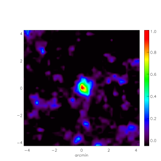
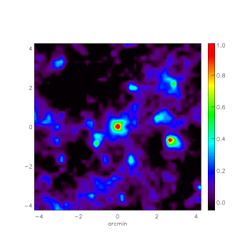
Figure 1: The convergence maps for isolated and non-isolated clusters as found in our simulations. The color bar shows the value of the (dimensionless) convergence $\kappa$.

2.2 Lensing by an Ideal Cluster

It is instructive to examine the lensing effect of an isolated cluster in the absence of other secondary anisotropies, foregrounds, instrument effects, or lensing by other structures, all of which we include later. If the deflections are small, we may expand the right hand side of equation (1) to linear order, so that

$$T(\mbox{\boldmath$\theta$})\approx\tilde{T}(\mbox{\boldmath$\theta$})-\delta\mbox{\boldmath$\theta$}\cdot\nabla\tilde{T}(\mbox{\boldmath$\theta$})$$ (9)

We will assume that equation (9) holds both here and in §3 for the purpose of illustrating some basic ideas. However, we note that this approximation is not actually necessary, and we shall dispense with it altogether in §4. It’s useful to consider the deflection angle due to a spherically symmetric cluster at comoving distance $\chi$

$$\delta\mbox{\boldmath$\theta$}=4G{(\chi_{s}-\chi)\over\chi_{s}\chi}{M(\theta)\over\theta}\mbox{\boldmath$\hat{\theta}$}$$ (10)

where $\theta$ $=(\theta_{x},\theta_{y})$ is now defined as the angular displacement from the center of the cluster, $\theta$ is the absolute value of $\theta$, and $M(\theta)$ is the mass of the cluster within a radius $\theta$. To first order, the cluster’s lensing effect is to remap the CMB radially away from its center, creating a step like wiggle in the CMB gradient centered on the cluster (?). We give an example of this behavior for a typical large cluster from our simulations in Figure (2). As expected from equation (9), the magnitude of the effect is proportional to both the local gradient of the CMB and the deflection angle along that gradient.

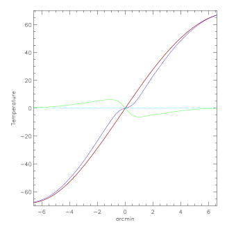
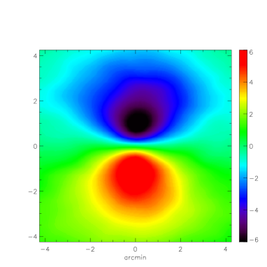
Figure 2: (left) A 1-d cut of the lensing signal $\Delta T(\theta)$ for a circularly symmetric ideal cluster lensing the CMB. The red line shows the unlensed CMB, the blue line shows the lensed CMB with the characteristic ‘kink’ near the origin and the green line shows the difference. (right) The signal in 2D for a circularly symmetric ideal cluster lensing a constant gradient. Note the dipolar nature of the lensing signal.

The lensing angle $\delta$$\theta$ cannot be solved for using equation (9) without more information; you can’t in general measure a scalar field and expect to solve for a scalar field and a vector field! If progress is to be made, some assumptions must be made about $\delta$$\theta$, $\nabla\tilde{T}$($\theta$), or both. We begin by noting that, in the absence of secondary anisotropies, the CMB is expected to have little power on small angular scales, so that $\nabla\tilde{T}$($\theta$) may be slowly varying in relevant regions near the cluster’s center. We examine this statement more carefully below, but for now we follow ? and make use of this idea to model the primordial CMB gradient in small regions near the cluster as a constant whose direction of steepest ascent can without loss of generality be taken as the y-axis, so that

$$\tilde{T}(\mbox{\boldmath$\theta$})\approx\tilde{T}_{y0}\ \theta_{y}$$ (11)

where $\tilde{T}_{y0}$ is the slope of the primordial CMB along the y-axis and we have ignored an overall constant.

We define the lensing signal due to a cluster $\Delta T$($\theta$) as the difference between the lensed and unlensed CMB temperature

$$\Delta T(\mbox{\boldmath$\theta$})\equiv T(\mbox{\boldmath$\theta$})-\tilde{T}(\mbox{\boldmath$\theta$})$$ (12)

Combining this with equations (9) and (11) and defining the deflection due to lensing by the cluster along the y-axis as $\delta\theta_{y}$ gives

$$\Delta T(\mbox{\boldmath$\theta$})\approx T(\mbox{\boldmath$\theta$})-\tilde{T}_{y0}\theta_{y}\approx-\delta\theta_{y}(\mbox{\boldmath$\theta$})\ \tilde{T}_{y0}$$ (13)

In Figure (2) we show $\Delta T$($\theta$) for a circularly symmetric isolated cluster lensing a constant gradient. The signal crudely resembles a dipole in appearance as you would expect from equation (9), though it falls off as $\sim M(\theta)/\theta$ away from the cluster as predicted by equation (10).

The lensing angle $\delta\theta_{y}$($\theta$) is not generally considered measurable because the original position of the background image isn’t known. However, far away from the cluster, the effect of lensing must be small, and the lensed and unlensed CMB must be roughly equal. If the approximation of equation (11) is valid at this distance, then it will be possible to measure $T$($\theta$) away from the cluster, determine $\tilde{T}_{y0}$, and solve for $\delta\theta_{y}$($\theta$). As we show in Figure (4), the convergence profile can be well reconstructed from this information. We note that the reconstruction is degenerate for density fluctuations that change $\delta\theta_{x}$ but don’t alter $\delta\theta_{y}$. This degeneracy is similar to that of the mass sheet degeneracy, but it applies to any line of constant density in $\Sigma$($\theta$) that happens to lie in the direction of the y-axis. We find the error due to this degeneracy to be quite small, and it is of course identically zero for a circularly symmetric cluster profile, where $\delta\theta^{2}=\delta\theta_{x}^{2}+\delta\theta_{y}^{2}$

It is clear from Figure (4) that reconstructing the convergence profile of a cluster from CMB temperature maps is certainly possible under the following highly artificial conditions:

• No foregrounds

• No instrument effects

• No CMB secondary anisotropies other than lensing

• The clusters are isolated

• The CMB is a pure gradient of constant slope

In §3, we begin to include these effects in the context of a toy model.

3 Results From a Toy Model

In this section, we make use of a toy model of cluster lensing of the CMB in order to investigate to what extent the issues raised in the bulleted points listed at the end of §2 will impact on our ability to reconstruct the convergence profiles of clusters using high resolution CMB temperature maps. We then present results from this toy model for two general cases: individual clusters and “stacked” average clusters.

3.1 Signal and Noise in the Toy Model

In the toy model, we assume that the primordial CMB in a small region near a cluster is a known quantity, which we then model as a gradient. This allows us to bypass the step of estimating the unlensed CMB from the actual maps (we address this issue in §4), which will be both lensed and noisy, and instead to directly measure the signal as defined in equation (12) plus a noise term $N$($\theta$), which includes all other effects, so that

$$\Delta T_{t}(\mbox{\boldmath$\theta$})\equiv\Delta T(\mbox{\boldmath$\theta$})+N(\mbox{\boldmath$\theta$})$$ (14)

where we define the measured signal in the toy model as $\Delta T_{t}$. According to equation (10), the deflection angle $\delta\theta\sim M(\theta)/\theta$, and from equation (13) the signal in any circular annulus is proportional to $\delta\theta$ times the slope of the CMB gradient $\tilde{T}_{y0}$ times the area of the annulus. Then the total signal to noise inside a circle of radius $\theta$ scales as

$${S\over N}\sim{\tilde{T}_{y0}\over\theta^{1\over 2}}\int d\theta M(\theta)$$ (15)

for Gaussian noise. Since the model relies on the approximation that the CMB gradient is constant (equation 11), which can only be valid on small scales, we have chosen to impose a cut-off radius of $4^{\prime}$ from the center of the cluster. That is, we assume a measurement of $\Delta T_{t}$ for $\theta<4^{\prime}$, and use no information at larger radii. We note that we do address the use of lensing information for reconstruction on larger scales elsewhere (?).

The toy signal $\Delta T_{t}$ is derived using an input convergence map made by ray-tracing through our N-body simulation. This convergence map is then used to make the deflection field $\delta\theta_{y}$ using Fourier methods, and $\Delta T$ is made by remapping $\tilde{T}$($\theta$^′) into $T$($\theta$) according to equation (1), where $\tilde{T}$($\theta$^′) is a gradient of constant slope. We provide a description of the N-body simulation and the creation of the convergence map in an appendix, and for now note only that the simulated clusters are in general neither isolated nor ideal, as can be seen in the convergence profiles of Figure (1).

After creating a map of the toy signal, we next introduce two noise components to the model. The first, the kinetic SZ, is highly correlated with the position of the cluster, and because it has the same spectral dependence as the CMB itself, it cannot be removed using multi-frequency measurements. We then add a Gaussian “white noise” component, which is uncorrelated with the location of the cluster, and can be thought of as instrument noise, and unless stated otherwise, we smooth with a $0.^{\prime}75$ beam (FWHM), such as is expected for APEX-SZ. We do not include noise sources which we expect to be small and uncorrelated with the cluster, such as other CMB secondaries, nor do we include point sources, dust, or the thermal SZ, which can in principle be removed or at least reduced by making use of their spectral dependence. In any real experiment, treatment of these effects will not be perfect, so excluding them entirely is somewhat optimistic.

3.2 Reconstruction of Cluster Profiles

In this section we address the issue of the reconstruction of cluster convergence profiles within the toy model both for individual clusters and “stacked” average clusters. We shall see that both instrument noise, and more perniciously the kinetic SZ, significantly degrade the reconstruction for individual clusters.

Let us begin by looking at the reconstruction including kinetic SZ for a typical large mass, high-$z$ cluster in Figure (3). Note that when the kinetic SZ is added the reconstruction is significantly altered, because some of the kinetic SZ signal is misinterpreted as lensing. This effect is particularly troublesome because it is spatially correlated with the lensing signal, spectrally indistinguishable from it, non-Gaussian, and only loosely correlated with the mass or thermal SZ signal from the cluster.

In the last panel of Figure (3), we show a reconstruction with no kinetic SZ but now instead including Gaussian random noise at a level of $3\,\mu$K-arcmin, roughly one third of that expected for the highest resolution maps from APEX-SZ and consistent with more ambitious future projects such as ACT and SPT. Even at this noise level, most of the features of the convergence map are lost, and it is evident that high quality reconstruction of cluster convergence maps for typical clusters is not achievable within the context of the experimental parameters we are considering. A strategy designed to integrate deeply on cluster locations would have to be adopted.

While the situation depicted in Figure (3) is typical, in some cases the kinetic SZ can be completely dominant, as we show in Figure (4). In this particular case the cluster happens to be rotating, so that the kinetic SZ signal has a dipole-like structure similar to that produced by lensing. Depending on the relative orientation of the kinetic SZ lobes and the direction of the CMB gradient, these signals can enhance or overwhelm the lensing signal. It is even possible to reconstruct a large negative convergence right at the cluster’s location!

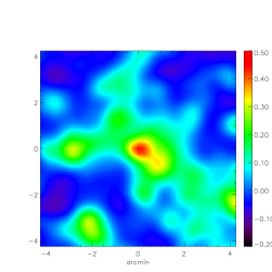
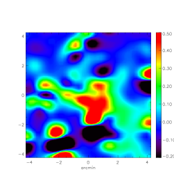
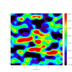
Figure 3: The reconstructed convergence maps for a typical cluster of $M_{200}=2.35\times 10^{14}\,h^{-1}M_{\odot}$ and $z=1$. We show the input map, the reconstruction with kinetic SZ, then with $3\,\mu$K-arcmin of instrument noise and no kinetic SZ.

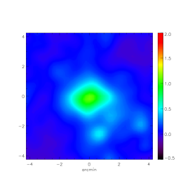
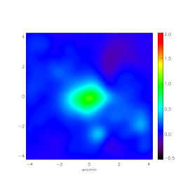
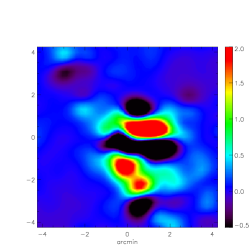
Figure 4: The convergence reconstruction for a large ($M_{200}=7\times 10^{14}\,h^{-1}M_{\odot}$), high redshift ($z=0.95$) cluster. The left panel is the true convergence smoothed by $0.^{\prime}75$, the center panel is the the reconstructed convergence using the toy model and no noise, and the right panel is the reconstructed convergence including the kinetic SZ. In this unusual case, the kinetic SZ dominates the reconstruction completely, causing the center of the cluster to appear as large and negative.

While this “disaster” cluster is clearly beyond hope, the reconstruction of a typical cluster might be improved if we mask out pixels which are likely to contain a large kinetic SZ component, which can be done by using the thermal SZ to roughly estimate the likelihood of a large magnitude kinetic SZ. This is essentially the idea proposed in ?. Figure (5) illustrates why this is not in general helpful; most clusters are not isolated, and many pixels must be excised. To make matters worse, the thermal SZ is not a perfect tracer of the kinetic SZ, so many perfectly good pixels are thrown away while others with large kinetic SZ signals are included.

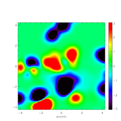
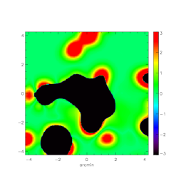
Figure 5: The kinetic SZ (left) for a typical (non-isolated) cluster and the thermal SZ (center) that you could try to use to mask it. The right panel is an example of a typical masked map, where the masked region is shown in black and the unmasked region is now (for clarity) the absolute value of the kinetic SZ. The thermal SZ is not a perfect tracer of the kinetic SZ, resulting in map with many perfectly good pixels removed, and residual kinetic SZ still included. The color bar in each case shows $\Delta T$ in $\mu$K.

Obviously, even if most clusters are not suitable candidates, we may be able to select some that are and focus on those. We have so far been thwarted in our reconstruction efforts by the kinetic SZ and instrument noise. If we ignore the latter for the time being, we realize right away that, although rare, clusters do sometimes form in relative isolation, as depicted in Figure (1). Perhaps these will be suitable?

Indeed, the level of contamination from the kinetic SZ is dramatically lower, and mostly associated with the cluster itself. We may now mask out the center of the cluster and have a reasonable expectation that the kinetic SZ contamination will be under control, and indeed that does prove to be the case here. However, we have specifically gone out of our way to select an isolated cluster, using the thermal SZ, and this has introduced a strong selection bias. The absence of other structures is marvelous for controlling the impact of the kinetic SZ, but the cluster is now located in a large void which dramatically reduces the projected mass below what one would expect from an average location. In essence we have introduced a mass sheet degeneracy. This is depicted in Figure (8). Here, we present the actual deflection angle along the y-axis. The dot-dash curve is the lensing angle that would result if the cluster were the only object in the universe, the solid line is the result including the cluster plus projection effects, and the dashed line is the actual deflection angle, where structures far away from the cluster of interest contribute to the deflection angle even though they don’t alter the convergence (this last is a degeneracy that arises because we have access only to the y-axis deflections). Thus, even though we “cheated” and simply used the y-axis deflection angle directly, rather than measuring it, we are still unable to reconstruct the clusters mass from this information due to a strong mass sheet degeneracy that in fact is consistent with a cluster mass estimate of zero at the virial radius, with absolutely no noise introduced, simply because of the confusion introduced from lensing by other structures.

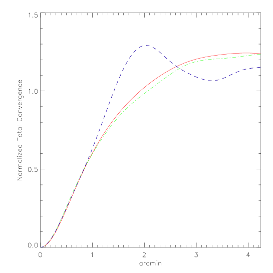
Figure 6: The cumulative convergence for our stack of 61 clusters with $2<M/10^{14}\,h^{-1}M_{\odot}<3$ and $1<z<1.5$ as a function of radius. Shown here are the input (red line), the reconstruction including kinetic SZ (green line), and reconstruction including kinetic SZ and noise (blue line).

Our investigation of the likely success of reconstruction of individual cluster mass profiles has shown that it will prove a more difficult problem than one might have hoped. It is worth noting that some of the difficulties we have encountered have come because we have used full field lensing and SZ simulations, rather than clusters that have been ‘cut out’ of simulations and then used to lens voids. Despite this technical difference though, our results so far are qualitatively in agreement with those of ?. They show in their Fig. 4 that they reconstruct the cluster mass to be essentially zero at the virial radius. We shall return to this point, and some of the reasons behind it, in the next section.

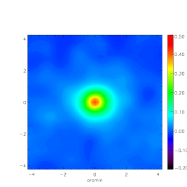
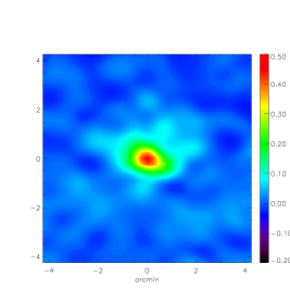
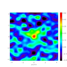
Figure 7: The convergence map (left) of our stack of 61 clusters with $2<M/10^{14}\,h^{-1}M_{\odot}<3$ and $1<z<1.5$, it’s reconstruction (center) including the kinetic SZ, and then again (right) with both Gaussian noise and kinetic SZ included.

Another approach, called stacking, is to consider a group of clusters binned according to relevant observables (e.g. temperature and redshift), cut out regions in the signal maps within a specified area centered on each cluster, stack them one on top of another, and then compute the average. The principal advantage of this technique is that essentially every unbiased source of confusion is reduced by this kind of averaging as $\sqrt{\rm N}$, where N is number of clusters used. This includes the important cases of the kinetic SZ, since the baryons are a priori equally likely to be moving toward or away from the observer, and of projection effects that proved so troublesome in the case of “isolated” clusters. If our cluster signal grows as $M$, our signal-to-noise is enhanced by stacking more relatively low mass clusters as long as the mass function is steeper than $M^{-2}$ per mass interval considered. This is the case for the high mass and redshift clusters we consider, suggesting we should target more lower mass clusters rather than fewer high mass clusters.

In Figure (7) we show the reconstruction of a stack made from 61 intermediate mass, high redshift clusters. First, consider the case where the only source of noise is the kinetic SZ. The convergence profile of the stack is circularly symmetric to a good approximation, which greatly reduces the mass line artifact that can arise in the reconstruction of finite fields, and it becomes feasible to reconstruct more of the central region. As in the case of single clusters, adding Gaussian instrument noise of $1.25\ \mu$K-arcmin to the stack (consistent with the anticipated $10\ \mu$K-arcmin for APEX-SZ averaged over 61 clusters) introduces substantial uncertainty to the convergence profile, but the total convergence as a function of radius is reasonably constrained, as can be seen in Figure (6). Thus, there is some promise that one might be able to provide reasonable mass estimates for cluster stacks, which might then be used to constrain the mass-temperature relation.

The reconstruction of cluster convergence profiles using weak lensing of the CMB is a technique that clearly shows promise for cluster stacks if the approximations of the toy model can be trusted. Some potentially important issues are not addressed by this simple model, the most important of which is the fact that the unlensed CMB is not a known quantity, so the signal as described in equation (13) is not directly measurable. We examine this issue in the next section.

4 Beyond the Toy Model

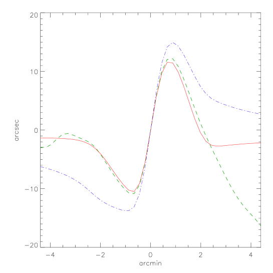
Figure 8: The deflection angles for an isolated cluster that occurred naturally in our simulations. The dot-dash line shows the deflection angle for the cluster if there were no other matter in the universe. The solid line shows the lensing from the projected convergence profile at the cluster’s location on the sky. Since lensing is dependent on the relative mass overdensity $\delta$, the void acts as a negative mass sheet. Finally, the dashed line is the actual deflection angle. Structures away from the center of the cluster do contribute to deflections, sometimes quite substantially.

In the previous section we showed that using high resolution maps of the CMB temperature to reconstruct stacked cluster convergence profiles is a technique that shows some promise when examined within the context of a simple toy model. By employing a toy model we have brushed aside a number of potentially important complications, perhaps the most glaring of which is having so far ignored the fluctuations intrinsic to the primordial CMB itself. Although our main focus in this section will be on stacked clusters, we nonetheless begin with some discussion in the context of individual clusters as a natural lead in to understanding this issue.

First recall the toy model ansatz of ? where the CMB temperature gradient can be approximated as constant over relevant length scales, and the CMB can be measured far from the cluster where the kinetic SZ and lensing by the cluster are both small. The unlensed CMB gradient can then be simply determined, as we illustrate in Figure (9), by ‘connecting the dots’ between the CMB on either side of the cluster. However, the CMB cannot be well approximated as a gradient on scales greater than a few arcminutes even for carefully selected portions of the CMB, so to use this technique to get a good fit for the unlensed CMB at the center of the cluster you are forced to set the lensing signal (and therefor the deflection angle) to zero at roughly a few arcminutes from the center of the cluster. Obviously the lensing effect of large clusters extends well beyond this range, so the ‘connect the dots’ method systematically underestimates the cluster’s mass (Equation 10) as you go farther from the cluster’s center, culminating in a total cluster mass estimate equal to zero on scales of a few arcminutes; that is, roughly at the virial radius. This is a completely generic feature of the method, and is easily seen in the second panel of Figure (9) or in Figure (4) of ?.

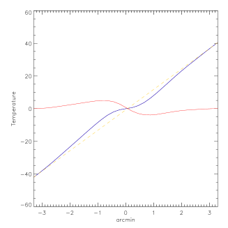
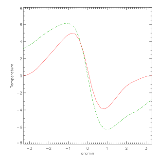
Figure 9: The lensing signal estimated using the ansatz of ? (Left) The lensed CMB (blue) is used as an estimate of the unlensed CMB on either side of the cluster, and the unlensed CMB (dashed orange) is estimated by connecting the dots. The difference between the two is then the estimate of the signal (red). (Right) A generic feature of this method of reconstruction is its systematic underestimate of the magnitude of the signal. The actual signal (dot-dash orange) is included for comparison.

A better method of estimating the unlensed CMB is certainly of interest. One obvious improvement is to extend on the original proposal of ? by making use of something other than a simple gradient. For example, one could fit the CMB far from the cluster with a second order polynomial (but note that nearby structure may cause problems). Alternatively, you could use a Wiener filter, as was recently suggested by ?. Unfortunately, although the fit is somewhat improved, these methods appear to suffer from the same drawback as the original, and lead to estimates of the virial mass that are systematically low and often consistent with zero.

A more sophisticated approach would be to iterate the fit or to include a model for both lensing and the unlensed CMB. This is the approach we take. Specifically we assume that the cluster is spherically symmetric and has an NFW profile, and we model the unlensed CMB locally as a 2nd degree polynomial in 2D (the above mentioned nearby structure contamination will average out when stacking). We consider a range of masses for the assumed NFW cluster and compute the lensing deflection angle for each. This is used to “delens” the CMB map. The resulting map which best fits, in the $\chi^{2}$ sense, a second degree polynomial (in 2D) is chosen. A second degree polynomial has the advantage of being even about the center of the cluster, while the lensing effect is odd, and on scales of a few arcminutes fitting an unlensed CMB fairly well. As a result, ‘bad’ fits will often be glaring.

We initially tested this method on clusters ‘cut out’ from simulations and with no instrument noise, kinetic SZ, etc., and were able to routinely estimate the mass to within 10%, and to within a few percent for our fiducial 61 cluster stack. However, the method incurs a bias toward underestimating the mass that becomes more significant as you include regions further from the center of the cluster. The bias occurs due to the failure of the 2D polynomial to accurately represent the CMB in the region around a cluster. One look at Figure (9) will convince the reader of the origin of the bias. The departure of the CMB from a constant gradient is also odd about the center of the cluster, so that while lensing by a cluster will degrade the ability of the polynomial to fit CMB near the cluster, it will actually help it fit better farther away, and the two effects compete. Given the need for as much usable area as possible to overcome other difficulties, it is likely that a 2D polynomial is ultimately not the best choice for the fit. One way to correct for this is to determine the expectation value of the odd component in the unlensed CMB and include this in the fitting procedure. Alternatively with enough clusters to beat down the kSZ contamination, a higher resolution, higher sensitivity observation would be able to work at smaller radius where the bias is much reduced.

5 Conclusion

In this paper we have investigated in some detail the promise of cluster lensing of the CMB. This idea was first introduced by ? and will soon become observationally feasible with the imminent commissioning of the APEX-SZ telescope. We verify that the method of Seljak & Zaldarriaga works well given their assumptions, but note that these assumptions are not well satisfied in practice.

In particular we highlight the role of the kinetic SZ signal as an important contaminant which is spatially correlated with the cluster and spectrally indistinguishable from the lensing signal itself. The kSZ fluctuations, being non-Gaussian and signal-correlated, are also an issue for reconstruction of large-scale structure as we discuss further in ?. If the unlensed CMB can be adequately estimated, we show that the stacked profiles and total masses are reasonably well constructed by CMB lensing, in contrast to profiles or masses of any individual cluster. We elucidate some of the issues in §4.

Finally we make some comments about the role of polarization in lensing. It has been emphasized before that the inclusion of polarization information can dramatically enhance the prospects for large-scale structure reconstruction from lensing of the CMB. This is because lensing induces a $B$-mode polarization signal which is otherwise absent for purely scalar, primary fluctuations. The large intrinsic signal, which is a source of ‘noise’ for lensing reconstruction, is thus absent.

It is possible that the addition of polarization information could enhance the prospects for cluster lensing also. To see whether the effects we have identified are mitigated by polarization information requires a detailed calculation. The signal levels for polarization are much smaller, and the spatial structure complicated as for temperature. The kSZ effect, which is one of our major contaminants, is also polarized. The dominant polarization signal comes in at order $\tau Q$ where $\tau$ is the cluster optical depth and $Q$ the local CMB intensity quadrupole at the location of the cluster. The resulting field is a mix of $E$- and $B$-mode signals with the polarization pointing in the direction of the quadrupole cold lobe. Depending on the variation of the quadrupole with distance and position in the field, and on the cluster properties the polarization signal can be somewhat complex. Near each cluster though it might be possible to significantly reduce the kSZ contamination through modeling. We leave a detailed investigation of this question to future work.

Acknowledgements:
C.V. would like to thank the organizers of the workshop “Cosmology with Sunyaev-Zel’dovich cluster surveys” held in Chicago in September 2003 for allowing him the chance to present some of this work. Additionally we would like to thank T. Chang, J. Cohn, D. Holz, B. Jain, A. Lee, G. Smoot, M. Takada and M. Zaldarriaga for helpful discussions about these results. The simulations used here were performed on the IBM-SP2 at the National Energy Research Scientific Computing Center. This research was supported by the NSF and NASA.

Appendix A The simulated map

We construct maps of lensing convergence and the thermal and kinetic SZ effect making use of a large, high-resolution N-body simulation of the $\Lambda$CDM cosmology (specifically Model 1 of ?). In this appendix we give some details of how this was done.

A.1 The N-body simulation

To construct the maps we need some information on the spatial distribution and evolution of the mass in our model. We obtain this from an N-body simulation. The simulation modeled a large volume of the universe, a periodic cube $300\,h^{-1}$Mpc on a side, to ensure a good sampling of the clusters of interest to us. We considered only the dark matter component which was modeled using $512^{3}$ particles of mass $1.7\times 10^{10}h^{-1}M_{\odot}$. For computation of the thermal and kinetic SZ effects we assume that any baryonic component would trace the dark matter, a reasonable approximation on the scales of interest to us.

The simulation was started at $z=60$ and evolved to the present using the TreePM code described in ?, with the full phase space distribution dumped every $100h^{-1}$Mpc between redshifts $2>z>0$. It is this range of redshifts which dominates the lensing and SZE signal on the angular scales of interest to us. The gravitational softening used is of a spline form, with a “Plummer-equivalent” (comoving) softening length of $20h^{-1}$kpc. All of the relevant cluster-scale halos contain several thousand particles to begin to resolve sub-structure. The simulation was performed on 128 processors of the IBM-SP2 at NERSC, took nearly 4000 time steps and approximately 100 wall clock hours to complete.

The maps were made in essentially the same manner as in ? to which we refer the reader for discussion of the various approximations. The past lightcone was constructed by stacking the intermediate stages of the simulation between redshifts $2>z>0$. In order to avoid multiply sampling the same large scale structures, each $300h^{-1}$Mpc box has been randomly re-oriented in one of the six possible orientations, and has furthermore been shifted by a random amount, perpendicular to the line-of-sight, making use of the periodic boundary conditions. There are three time dumps per box length. Each $300h^{-1}$Mpc volume in the stack is made up of three segments, each segment evolved to a later epoch than the previous one by the time it takes light to travel $100h^{-1}$Mpc. We chose $100h^{-1}$Mpc as the sampling interval because it is large enough that edge effects are minimal, yet fine enough that the line of sight integrals are well approximated by sums of the (static) outputs. Because of the periodicity, we are free to choose any of the thirds as the oldest, cyclically permuting the other two. This approach preserves the continuity of large-scale structure over distances of $300h^{-1}$Mpc without compromising the resolution in time evolution.

We produced maps of the lensing and SZ effects. Each map was $7.5^{\circ}$ on a side, with $2048^{2}$ square pixels each $0.22^{\prime}$ on a side. The same particle distribution and random seeds were used to construct each of the maps, so that they represent the same patch of sky in each quantity. We now discuss each map in turn.

A.2 Convergence ($\kappa$) maps

The effect of lensing was computed from maps of the convergence, $\kappa$, assuming the weak lensing approximation (see §2). This is valid except near the very center of the cluster, and so adequate for our purposes. The convergence was computed from the density contrast along the past lightcone as

$$\kappa={3\over 2}\Omega_{\rm mat}H_{0}^{2}\int d\chi\ g(\chi){\delta\over a}$$ (16)

where $g(\chi)=\chi(\chi_{s}-\chi)/\chi_{s}$ is the lensing kernel, $\chi$ is the comoving distance and $\chi_{s}\simeq 9\,h^{-1}$Gpc is the comoving distance to the last scattering surface. We have assumed the universe is spatially flat. The (projected) density contrast within each $100\,h^{-1}$Mpc slice was computed from the dark matter distribution using a spline kernel interpolation with a smoothing length equal to the force softening in the simulation.

A.3 Compton-$y$ and $b$ maps

Because the simulation contains no gas we use a semi-analytic model to include the gas physics. First we assume that the gas closely traces the dark matter. This is likely a good approximation in all regions except the innermost $O(100)$kpc of the cluster, which for clusters at cosmological distances will be unresolved by the experiments of interest. (e.g. $100$kpc subtends only $0.26^{\prime}$ at $z=0.5$.) We ignore the presence of cold gas and stars in the ICM, assuming that the mass in hot gas is $\Omega_{\rm b}/\Omega_{\rm m}$ of the total. Second, each cluster is assumed isothermal. We assign to each particle in a group a temperature proportional to its mass to the $2/3$ power.

We generate Compton-$y$ maps by integrating for each pixel

$$y=\int\sigma_{\rm T}n_{e}{k_{\rm B}T_{e}\over m_{e}c^{2}}dl\qquad.$$ (17)

Here $\sigma_{\rm T}$ is the Thompson scattering cross section, and $n_{e}$, $m_{e}$ and $T_{e}$ are the electron number density, mass and temperature respectively. We assume that within the clusters the gas is fully ionized. The contribution from each particle is distributed over the pixels with a spline weighting and a size equal to the smoothing length of the simulation as for the $\kappa$ maps above. The temperature fluctuation at frequency $\nu$ is then obtained from the $y$-maps by

$${\Delta T\over T} = \phantom{-2}y\left(x{{\rm e}^{x}+1\over{\rm e}^{x}-1}-4\right)$$ (18)

$$\simeq -2y\qquad\mbox{for }\ x\ll 1\,,$$ (19)

where $x=h\nu/k_{B}T_{CMB}\simeq\nu/56.84$GHz is the dimensionless frequency and the second expression is valid in the Rayleigh-Jeans limit. In what follows we shall assume the low-frequency limit unless otherwise stated.

The Compton-$b$ maps are produced in an almost identical manner, replacing $kT/m_{e}c^{2}$ with $v/c$, where $v$ is the line-of-sight velocity. The spectrum is an undistorted black body, so the temperature perturbation is simply $\Delta T/T=-b$.

A.4 Primary CMB anisotropies

When needed we generate primary CMB anisotropies as a random realization of a Gaussian field with power spectrum computed from CMBfast (?). We generate random phases in momentum space, and assign amplitudes to each of the $k$-modes using a distribution whose average value is the amplitude in the CMB power spectrum. We have used the flat sky approximation, in which the $k$-mode in momentum space corresponds to $\ell$ value in the CMB power spectrum.

References

- [1]
- [2] [] Amblard, A., Vale, C., White, M., 2004, in preparation
- [3]
- [4] [] Bennett C.L., et al., 2003, ApJS, 148, 1 [astro-ph/0302208]
- [5]
- [6] [] Bartelmann, M., & Schneider, P., 2001, Phys. Rep., 340, 291-472
- [7]
- [8] [] Bartelmann M., 2003, preprint [astro-ph/0304162]
- [9]
- [10] [] Birkinshaw M., 1999, Phys. Rep., 310, 98
- [11]
- [12] [] Cooray, A., 2003, ApJ, 596, L127
- [13]
- [14] [] Hirata, C. M., Seljak, U., 2003, Phys.Rev.D, 67, 43001
- [15]
- [16] [] Holder, G., & Kosowsky, A., 2004, preprint [astro-ph/0401519]
- [17]
- [18] [] Hu, W, 2001, ApJL, 557, L79
- [19]
- [20] [] Jain B., Seljak U., White S.D.M., 2000, ApJ, 530, 547 [astro-ph/9901191]
- [21]
- [22] [] Metzler C., White M., Loken C., 2001, ApJ, 547, 560 [astro-ph/0005442]
- [23]
- [24] [] Okamoto, T., Hu, W.,2003, PhysRevD, 67, 83002
- [25]
- [26] [] Reblinsky K., Bartelmann M., 1999, A&A, 345, 1
- [27]
- [28] [] Rephaeli, Y., 1995, ARA&A, 33, 541
- [29]
- [30] [] Schulz A., White M., 2003, ApJ, 586, 723 [astro-ph/0210667]
- [31]
- [32] [] Seljak U., Zaldarriaga M., 1996, ApJ, 469, 437 [astro-ph/9603033]
- [33]
- [34] [] Seljak, U., Zaldarriaga, M., 1999, Physical Review Letters, 82, 2636
- [35]
- [36] [] Seljak, U., & Zaldarriaga, M., 2000, ApJ, 538, 57-64 (2000ApJ...538...57S)
- [37]
- [38] [] Sunyaev R.A., Zel’dovich Ya. B., 1972, Comm. Astrophys. Space Phys., 4, 173
- [39]
- [40] [] Sunyaev R.A., Zel’dovich Ya. B., 1980, ARA&A, 18, 537
- [41]
- [42] [] Vale C., White M., 2003, ApJ, 592, 699 [astro-ph/0303555]
- [43]
- [44] [] White M., 2002, ApJS, 143, 241 [astro-ph/0207185]
- [45]
- [46] [] Yan R., White M., Coil A., 2004, ApJ, in press [astro-ph/0311230]
- [47]
- [48] [] Zaldarriaga,M., Seljak, U., 1999, Phys.Rev.D, 59, 123507
- [49]
- [50] [] Zhang, P., Pen, U., Trac, H., 2003, [astro-ph/0304534]
- [51]