Spectro-photometric and weak lensing survey of a supercluster
and typical field region – I. Spectroscopic redshift measurements

Abstract

We present results from a spectroscopic study of $\sim$4000 galaxies in a $\sim 6.2$ deg² field in the direction of the Aquarius supercluster and a smaller typical field region in Cetus, down to $R<19.5$. Galaxy redshifts were measured using the Two Degree Field system on the Anglo-Australian Telescope, and form part of our wider efforts to conduct a spectro-photometric and weak gravitational lensing study of these regions. At the magnitude limit of the survey, we are capable of probing $L_{*}$ galaxies out to $z\sim 0.4$. We construct median spectra as a function of various survey parameters as a diagnostic of the quality of the sample. We use the redshift data to identify galaxy clusters and groups within the survey volume. In the Aquarius region, we find a total of 48 clusters and groups, of which 26 are previously unknown systems, and in Cetus we find 14 clusters and groups, of which 12 are new. We estimate centroid redshifts and velocity dispersions for all these systems. In the Aquarius region, we see a superposition of two strong superclusters at $z=0.08$ and $z=0.11$, both of which have estimated masses and overdensities similar to the Corona Borealis supercluster.

1. Introduction

Over the past few years our understanding of the large scale distribution of galaxies has advanced greatly. With current spectroscopic surveys of the local galaxy population ($z\sim 0.1$), such as the 2dF Galaxy Redshift Survey (2dFGRS; Colless et al. 2001) approaching 250,000 galaxies, and the ongoing Sloan Digital Sky Survey (SDSS; Strauss et al. 2002) set to capture the spectra of a million galaxies, statistical errors on key quantities of interest are fast becoming diminutive. A major goal of these surveys is to make accurate measurements of the large-scale distribution of matter density fluctuations in the Universe and so measure the cosmological parameters.

However, since one is not probing the matter directly, but instead some population of objects that merely trace the mass, e.g., galaxies of a particular luminosity class, spectral type etc…, it is necessary to make some assumptions about the way in which these two distributions are related – or more commonly biased. In recent work (Tegmark et al. 2004; Percival et al. 2004), it is assumed that there is a certain large scale, $\sim 20h^{-1}$Mpc or so, above which the galaxy tracers and mass are related by a simple scale independent constant bias. Whilst this may indeed turn out to be correct, it is important to establish the veracity of this assumption through direct observation, if redshift surveys are to be trusted as precision cosmological probes.

Weak gravitational lensing provides the most exciting progress towards solving this problem. The weak distortions in the shapes of faint background galaxies due to the gravitational deflection of light bundles as they travel through distorted spacetime provides a direct probe of the projected mass distribution (e.g., Kaiser 1992; Kaiser & Squires 1993). More recently Bacon & Taylor (2003) and Taylor et al. (2004) have shown that if one has redshift information for all galaxies, then one may also reconstruct the 3D mass distribution.

Also, Schneider (1998) has developed a method for exploring the bias. This has been applied by Hoekstra et al. (2001, 2002), who found on scales $<5h^{-1}$Mpc, that the bias was scale-dependent, with positive bias on scales $<0.25h^{-1}$Mpc, anti-bias on scales $\sim 1h^{-1}$Mpc and almost no biasing at the limits of their survey. If all of the systematics in this work are under control, then this is strong support for the ‘Concordance cosmology’ (Wang et al. 2000), which requires bias of this kind to match the galaxy clustering statistics (Benson et al. 2000; Peacock & Smith 2000).

A complicating factor in the analysis is that the lensing effect depends on the geometry of the system and one therefore requires knowledge of the spatial distribution of the lens and source galaxy populations to obtain accurate measurements. However, as Hoekstra et al. (2001, 2002) have shown, if one has redshift information for the lens galaxies only, then one may make good progress through assuming an appropriate redshift distribution for the background lens galaxies.

In a series of papers, we perform a combined weak lensing and spectro-photometric study of a supercluster and also a control field region with the specific aim of uncovering detailed information about bias over a wide range of scales and environments. We intend to bridge the gap between having no and full spatial information along the light cone, by measuring spectra for the foreground galaxies. In this, the first paper of the series, we present the spectroscopic part of the survey. In a subsequent paper we will describe our deep photometric and weak lensing analysis of the regions, and in a further paper we will combine all of the data to directly answer the above questions.

Using the 2dF instrument on the AAT we have measured the spectra for a significant fraction of all galaxies in the survey regions, down to $R<19.5$. From these data we determine redshifts through cross-correlating each spectrum with a set of standard galaxy and stellar templates. We then determine the redshift space distributions for the two survey regions, finding marked differences between them. As a by-product of this work, we have used the full redshift space sample to compile new lists of cluster candidates for the regions, and this is the subject of the latter part of the paper. For these cluster candidates we estimate redshifts and velocity dispersions.

The paper is broken down as follows: In § 2, we describe the survey and the spectroscopic target catalogs. In § 3, we describe the observations and data reduction. In § 4, we describe the redshift estimation procedure and then present some interesting properties of the spectroscopic sample. In § 5 we use the sample to establish clusters within the survey. Here, we also provide an updated cluster catalog for the Aquarius region. In § 6 we give estimates of the centroid redshift, velocity dispersion and asymmetry index of each cluster candidate. Finally, in § 8, we discuss our findings and summarize the results. Throughout this paper we have assumed concordance cosmology (Wang et al. 2000) with $\Omega_{m}=0.3$, $\Omega_{\Lambda}=0.7$, where $\Omega_{m}$ and $\Omega_{\Lambda}$ represent the matter and vacuum energy density parameters at the present epoch. All celestial coordinates are given for epoch J2000.0.

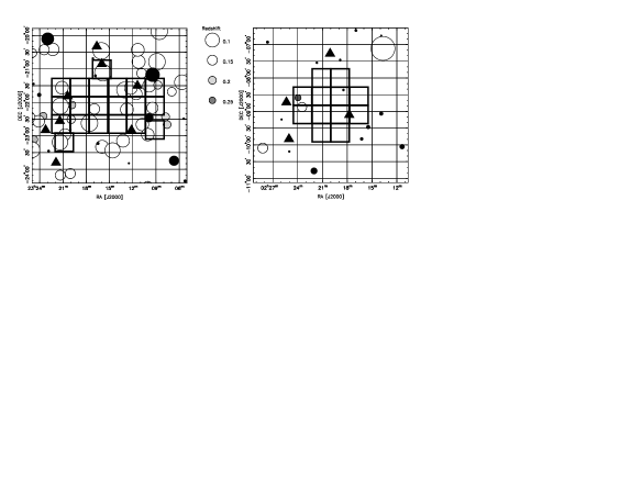
Figure 1.— Survey regions. The left panel shows the Aquarius supercluster region and the right panel shows the typical field region in Cetus. In both panels the contiguous thick square tiles correspond to the field of view of the WFI camera ($33^{\prime}\times 34^{\prime}$), and de-mark the survey boundaries. Overlaid on both plots are known clusters; those that have had redshifts measured are represented by circles, where the size and shading of the circle is in proportion to the Abell radius and redshift of the cluster; and those with no previous redshift estimate are identified as triangles. Filled black circles represent field stars brighter than $V=8.0$, where the size of the circle increases with increasing brightness.

2. Survey Description

The survey comprises deep photometric imaging and spectroscopy in two regions: the supercluster in the direction of Aquarius [$\alpha=23^{h}15^{m}$, $\delta=-22^{\circ}$], which is of general interest; and a typical field region in Cetus [$\alpha=02^{h}19^{m},\delta=-8^{\circ}50^{\prime}$]; hereafter referred to as the Aquarius and Cetus regions. The Cetus region was chosen to coincide with one of the SDSS southern strips. In the future this will provide us with additional multi-colour photometry and spectra. The deep photometric observations are being carried out on the ESO 2.2m telescope at La Silla, using the Wide Field Imaging Camera (WFI) and the spectroscopy is being carried out using the 2dF multi-fiber-object spectrograph on AAT.

The Aquarius supercluster was firmly established by Batuski et al. (1999), previously being noted as one of the highest concentrations of rich clusters on the sky (Abell 1961; Murray et al. 1978; Ciardullo et al. 1985; Abell, Corwin & Olowin 1989,  hereafter ACO). From spectroscopy, Batuski et al. deduced that the core of the supercluster contained five richness class $R\geq 1$ ACO clusters: A2546 (catalog ), A2554 (catalog ), A2555 (catalog ), A2579 (catalog ) and A3996 (catalog ); making the Aquarius supercluster even denser than the most massive superclusters at lower redshifts, such as the Shapley supercluster (Raychaudhury 1989) and the Corona Borealis supercluster (Postman, Geller & Huchra 1986). More recently a study of the region was undertaken by Caretta et al. (2002,  hereafter Caretta02), who used projected galaxy distributions and follow-up spectroscopy to compile a list of 102 cluster candidates over $\sim$80 deg². There also exists archival Chandra and/or ASCA data for 10 of the Aquarius clusters.

Fig 1 presents the survey regions. The Aquarius field comprises 20 overlapping WFI pointings, covering an angular area of $\sim$6.2 deg², which at the median redshift of the spectroscopic survey, ($\bar{z}\sim 0.176$), corresponds to scales of the order 30 $h^{-1}$ Mpc $\times$ 15 $h^{-1}$ Mpc. Out to the effective limit of the survey $(z\sim 0.45)$, the comoving volume surveyed in the Aquarius region is $1.0\times 10^{6}h^{-3}$Mpc³. The Cetus field comprises 12 overlapping WFI pointings, covering an angular area of $\sim$3.7 deg², which again at the median redshift of the spectroscopic survey corresponds to transverse scales 20 $h^{-1}$Mpc $\times$ 20 $h^{-1}$ Mpc; and out to the effective survey limit, a comoving volume of 5.6 $\times 10^{5}\,h^{-3}$Mpc³.

Within the Aquarius fields we have identified 23 known clusters (Caretta02), 5 of which have no redshift estimate. This corresponds to an average surface density of 3.7 clusters deg^-2. In contrast, the Cetus region was chosen to contain only one Abell cluster, which had a richness class $R=0$ and distance class $D=6$. This gave an average 0.27 clusters deg^-2. Since the mean surface density of Abell clusters over the whole sky is $\sim$0.2 clusters deg^-2, we are justified in our assertion that the Cetus region is indeed a ‘typical’ patch of sky. We note that there is an additional known cluster, RX J0223.4-0852 (catalog ), within the field, and an Abell cluster, A348 (catalog ) ($z=0.27$), that glances the Eastern edge of our 2dF survey region.

2.1. The Spectroscopic Input Catalog

The spectroscopic targets were taken from the SuperCOSMOS on-line catalog (Hambly et al. 2001a). We selected all objects down to a magnitude limit of $R\leq 19.5$. For $R\leq 19$, the image classification is $>90\%$ reliable and for $R\leq 19.5$ this drops to $>80\%$ (Hambly et al. 2001b). On inspecting the data we found that faint satellite trails still remained in the catalog. These were removed by matching objects from the $R$ and $b_{J}$ plates, which were observed at separate epochs. The astrometry of the SuperCOSMOS R-band data has a measured positional accuracy to better than $\pm 0.2\arcsec$ at $R\sim 18$, deteriorating to $\pm 0.3\arcsec$ at $R\sim 21$ (Hambly et al. 2001b), and this was of sufficient accuracy for the requirements (2$\arcsec$ fiber diameters) of the 2dF instrument. We then corrected the $R$ magnitudes for absorption using the dust maps of Schlegel, Finkbeiner & Davis (1998). For the Aquarius region we used an extinction correction $A_{R}\sim 0.074$, and for Cetus we used $A_{R}\sim 0.07$.

Taking $M_{*r}-5\log_{10}h=-20.83$ (Blanton et al. 2003), then for galaxies at the flux limit of our survey ($R=19.5$) we are capable of probing $M_{*}$ galaxies out to $z\sim 0.4$, or equaivalently angular diameter distances of $\sim 1$Gpc, where we have assumed a $K$-correction $\sim 0.5$ (Coleman, Wu & Weedman 1980).

To acquire spectra of sufficient quality for precise redshift estimation, we followed the 2dFGRS strategy and aimed to obtain spectra with a minimum signal-to-noise ($S/N$) $\sim$10. For galaxies with a $S/N$ of this order, Colless et al. (2001) found a redshift completeness $>90\%$. For objects at the survey flux limit and and in poor seeing conditions, we estimated that these $S/N$ levels could be reached for 6500 s integrations. However, for galaxies one magnitude brighter, a similar $S/N$ was achieved in roughly half the time. To optimize the use of telescope time, the spectroscopic observations were split into two sets: short exposures for bright ($R<18.5$) galaxies; and longer exposures for faint ($19.5<R\leq 18.5$) galaxies. Fig.2, top panel, presents the input catalog for the bright Aquarius galaxies and the bottom panel shows the faint. For the Aquarius catalogs we identified $3441$ bright galaxies and $5246$ faint. Similarly, for the Cetus region catalog we identified $1414$ bright galaxies and $1881$ faint.

Figure 2.— Source catalogs for the survey. Top panel shows all galaxies in the survey region with ($R<18.5$) and bottom panel shows all galaxies with ($19.5>R\geq 18.5$). Overlaid thick grid represents the fields that have been selected for deep $R$ band imaging using the WFI camera. Also overlaid are the 2dF fields (large circles).

3. Spectroscopic Observations and Analysis

3.1. Fiber Configurations

For the Aquarius field, six overlapping 2dF pointings were chosen to cover the target area, and for the Cetus field, the whole target area was contained within a single 2dF centre. Owing to the high surface density of sources, $\sim$1400 deg^-2 in the Aquarius region and $\sim$1048 deg^-2 in the Cetus region, multiple 2dF pointings of each of the chosen centres were required to target all of the galaxies in each field. In full operational mode the 2dF is capable of acquiring the spectra of 400 objects simultaneously. The fiber arrangements for individual fields were pre-configured using the observatory supplied software package CONFIGURE. For a full description of the 2dF instrument and configuring for dense fields see Bailey, Glazebrook & Bridges (2002, hereafter BGB02).

For the bright galaxy fields we typically allocated 360 fibers to target objects and 40 to sky (20 per spectrograph). For the faint galaxy fields we increased the allocation of sky fibers to 30 per spectrograph. This increase was to ensure accurate sky subtraction for the faint spectra. We discuss this further in § 3.3. Also as part of our allocation strategy, there was a small chance that a few objects would be re-observed. As we describe later in § 3.4, this small number of repeat observations enabled a useful test of the redshift estimation procedure.

3.2. Observing

Observations were carried out between October 29 and November 2, 2002 at the AAT. The 2dF spectrographs were configured with the 316R and 270R gratings. This pair gave FWHM resolutions of 8.5 and 9.0 Å per pixel, respectively, and an efficiency $>70\%$ for the wavelength range 5000-8500 Å. For the bright catalog galaxies, individual pointings comprised: calibration frames, consisting of a tungsten lamp flat field exposure, followed by a CuHe+CuAr arc lamp exposure; $3\times 1000$ s exposures of the target field. The target spectra were acquired as a series of snapshots to facilitate the removal of cosmic rays. For the faint catalog galaxies, the procedure was identical except that 5$\times$1300 s exposures were taken and also a further arc lamp calibration was taken at the end of the observation. In total, we acquired 6800 target spectra.

3.3. 2dF Data Reduction

All data reduction was performed using the latest version of the AAO-supplied software package 2dFDR-V2.3 (for details, see BGB02). In brief, the reduction recipe that we adopted was as follows: The data were de-biased. Bias strips were trimmed from the data frame and the mean of these was subtracted from the data. The fiber-flat field frame was then used to generate tram-line maps for the data. Since the accurate determination of these was crucial to achieving reliable reduction, they were carefully inspected at each stage in their generation.

The spectra were then extracted using the FIT routine, which performs an optimal extraction based on fitting overlapping Gaussian profiles to a fiber flat-field frame. The extracted data were then flat fielded using the fiber flat field data and re-binned onto a uniform linear wavelength scale, with the wavelength calibration for each fiber being determined from the closest in time CuHe+CuAr arc lamp exposure. The relative throughput of each fiber was then determined and the median sky generated and subtracted from each spectrum. Since good determination of the relative fiber throughput and sky subtraction was crucial for the faint galaxy spectra, we considered this carefully. We found that through using the Skyflux(cor) routine in the 2dF reduction package, we were able to produce good throughput calibration, and perform sky subtractions to an accuracy $\sim 1.5-3.0\%$. These accuracies are comparable to those obtained by Willis, Hewett & Warren (2001). In Fig. 3, we show the median sky and residual sky for all of the faint galaxy exposures. The residual sky was constructed by subtracting the median sky spectrum from each of the individual sky fibres and then calculating the median spectrum of these sky-subtracted sky fibres. This clearly demonstrates that the sky subtraction method that we have adopted is accurate. For the bright data the overall sky subtraction was of similar quality. Finally, the reduced runs were optimally combined and cosmic ray events were removed using a $5\sigma$-clipping rejection criterion.

Figure 3.— Top panel shows the median sky spectrum. Bottom panel shows the median residual sky (solid line) and the mean$+1\sigma$ residual sky (dotted line), determined from all of the sky fibers in the deep exposure frames.

Figure 4.— Comparison of redshifts for targets with repeated observations in the Aquarius region (top panel) and the Cetus region (middle panel). The bottom panel shows targets with previously measured redshifts. Plotted are the velocity difference $\Delta(cz)$ as a function of the mean redshift of the two observations $<z>$. In all panels, the points represent spectra for which both of the estimated qualities were, $Q\geq 3$. The dash lines represents the rms variation.

Figure 5.— Selection of rest frame spectra. The panels on the left show spectra from the bright ($R<18.5$) survey and those on the right show spectra from the faint ($19.5>R\geq 18.5$) with redshifts ($0.15<z<0.25$). Going from top to bottom shows changes in quality, with top panels representing $Q=5$, middle $Q=4$ and bottom $Q=3$. The short thin lines at the top of each figure denote interesting absorption/emission features.

3.4. Redshift Estimation

Redshifts were measured using a modified version of the CRCOR code developed for the 2dFGRS (Colless et al. 2001). This uses both cross-correlation against template spectra (Tonry & Davis 1979) and identification of emission lines to estimate the redshift for each galaxy. The set of templates used for this analysis was the same as presented by Colless et al. (2001). Each redshift estimate was visually checked against the galaxy spectrum, and a quality flag, $Q$, was assigned according to the reliability of the estimate. This reliability assessment was arrived at through considering the cross-correlation $R$ value and the number of identified emission lines. The value of $Q$ assigned to each estimate was between 1-5, with 1 being no confidence and 5 being extremely confident. In all our later analysis we use only galaxies with $Q\geq 3$. Of the 5875 target objects observed, 3841 had $Q\geq 3$. Of these 1245 were $Q=3$, 2251 were $Q=4$ and 345 were $Q=5$. Note that poor weather observations, for which only a handful of spectra were measurable, have also been included in this accounting.

During the observing run, 15 galaxies in the Aquarius field and 121 galaxies in the Cetus field were targeted twice. These repeats provided a useful test of the redshift estimation process. In Fig. 4, we plot the difference in recession velocity, $\Delta(cz)=c(z_{1}-z_{2})$, between the two estimated redshifts as a function of the mean redshift $\left<z\right>$ of the pair. For the Aquarius field (Fig. 4, top panel), of the 15 repeats, 10 of the redshift estimates agreed very well with an rms error of 67  km  s^-1. For four of the cases one of the observations was of poor quality $Q<3$, so that the comparison was unreliable and we do not show these. However, for one of the repeats, the estimates disagreed by $\Delta(cz)\sim 15,000\,{\rm km\,s^{-1}}$, and the quality flags were 3 and 4. We then inspected this erroneous pair to ascertain whether or not it was a genuine ‘blunder’.

Inspecting the images from the SuperCOSMOS archive we found two sources separated by less than 2$\arcsec$. Owing to the strong likelihood that the spectrum is composite, we were unable to trust the spectral features. For the Cetus field region (Fig. 4 middle panel), of the 121 repeats, 70 of the pairs had at least 1 galaxy with $Q<3$. These we did not consider further. Of the remaining 51, we found 11 pairs with a velocity difference greater than 300  km  s^-1. Inspecting these closer, we found evidence for 3 having close companions. Excluding these from the sample we then found an rms error of 153  km  s^-1.

A further test of the redshift estimation procedure was performed by comparing our sample with overlap galaxy redshifts extracted from the NED . From this archive we found 42 literature redshifts that overlapped with our Aquarius survey region. No redshifts were available for the Cetus region. Fig. 4 (bottom panel) shows the velocity differences from this comparison. For these data we initially found an rms error of $\sim 4000$  km  s^-1. However, on identifying and removing a single observation for which $\Delta(cz)=26,400$  km  s^-1, we found that the rms dropped to $\sim 160$  km  s^-1. For this NED galaxy, we traced the redshift measurement to the work of Colless & Hewett (1987), who reported that the estimate for this object was not safe and was rejected from their analysis. This leads us to conclude that our overall blunder rate for measuring redshifts is low.

4. Characterizing the Sample

4.1. The Rest-frame Spectra

Fig. 5 presents a selection of ‘early-type’ rest frame galaxy spectra with redshifts around the median for the survey, $(0.15<z<0.25)$. These were generated by linearly interpolating over important sky absorption bands, de-redshifting each spectrum and then linearly interpolating it on to a uniform wavelength scale with range 3500Å$<\lambda<$7000Å and pixel scale 5.83Å per pixel.

Figure 6.— The mean and median $S/N$ rest-frame galaxy spectra of the sample. The top panel presents the median (solid line) and mean (dotted line) galaxy spectrum for all of the galaxies with $Q\geq 3$. The middle panel presents the median galaxy spectra for the three different quality classes. The bottom panel presents the median galaxy spectra that result when the galaxies are divided into bins in magnitude: $19.5\geq R>19$; $19\geq R>18$; and $18\geq R$.

Figure 7.— The median rest-frame spectra by redshift. The galaxy sample has been split into three bins in redshift space these are: all galaxies $z\leq 0.1$ (top panel); all galaxies with $0.1<z\leq 0.2$ (middle panel); all galaxies $z>0.2$ (bottom panel).

We now calculate the mean and median signal-to-noise rest-frame spectrum as functions of quality class, magnitude and redshift as diagnostics for the sample. Fig. 6, top panel, shows the mean and median $S/N$ spectrum for galaxies with $Q\geq 3$. For both mean and median, the general shape of the spectrum is close to that of an early-type galaxy, but with emission lines superposed. Furthermore, the average galaxy spectrum in the sample has a $S/N$ better than 10.

Fig. 6, middle panel, shows the median spectrum by quality class. It is apparent that nearly all of the features in the high quality spectra are discernible in the lower quality spectra, but with lower strength absorption and emission features. Quantitatively, the $Q=3$ and $Q=4$ spectra possess a $S/N$ level a factor of $\sim 4$ and $\sim 2$ lower than the $Q=5$ spectra.

Fig. 6, bottom panel, shows the result of splitting the sample into three bins in magnitude: $R\geq 19.0$; $19.0>R\geq 18.0$; and $R<18.0$. For the brightest two bins, the median spectral energy distributions are better than $S/N=10$, but for the fainter bin galaxies the $S/N$ is lower, being $\sim 6$. This indicates that these objects are only just being detected. However, there is clear evidence of characteristic emission and absorption features, which indicates that for most cases, the correct redshift has been assigned to these galaxies. The absence of H_α emission can be attributed to two effects: The first is that the faint objects are predominantly at higher redshifts and so have had the red part of their spectrum redshifted out of the frequency bandwidth for our observations; the second is that since our sample contains a large number of low-redshift clusters we are preferentially biased to observing low-luminosity cluster ellipticals.

Finally, in Fig. 7, we consider the median by redshift. We have split the sample into three bins in redshift: $z\leq 0.1$; $0.1<z\leq 0.2$; $z>0.2$. Considering the first redshift bin, $z\leq 0.1$, the median spectrum is of high $S/N$, is flatter than a typical early-type spectrum, and has weak absorption features and fairly strong emission lines. The median spectrum for the next redshift bin, $0.1<z\leq 0.2$, again is of good $S/N$, is similar to an early type spectrum but with emission lines superposed. For the highest redshift bin, $z>0.2$, we find that the median spectrum shows strong characteristics of being an early-type galaxy, but with strong O II and O III emission features. Again, the absence of H_α emission can be understood from the arguments discussed above. It is possible that some of this evolution of the median spectrum with redshift may be due to true evolution in the galaxy populations. However, it is more likely due to selection effects. Since the Aquarius fields are cluster rich, we should expect a large number of cluster ellipticals in the intermediate redshift bins, whereas for the low redshift bins, we expect a more even mix of early- and late-type galaxies. Owing to the flux limit, the higher redshift bin will be dominated by bright ellipticals and also bright spirals, which accounts for the strong emission line and absorption features.

Figure 8.— Cone plot for Aquarius region. This shows all galaxies with $Q\geq 3$. Circles indicate cluster candidates from §5, where sizes are scaled by the estimated velocity dispersion (see Table 1).

Figure 9.— Similar to figure 8, but for the Cetus region.

Figure 10.— Redshift distributions of the galaxies with $Q\geq 3$. The top panel represents the total redshift distribution for all of the galaxies in the two regions; the middle panel, the galaxy distribution in Aquarius; and the bottom panel the galaxy distribution in Cetus. The dash line in each panel corresponds to an analytic fit to each distribution.

4.2. Spatial Distribution

Figs 8 and 9 show the cone plots for all galaxies with $Q\geq 3$ in the Aquarius and Cetus field regions, respectively. In order to show the large-scale structure more clearly, the right ascension direction of the plots has been stretched out by a factor of 10 and thus the apparent transverse filamentary features should be viewed circumspectly. Nevertheless, it is clear that there is strong clustering in the distribution of galaxies. In particular, the Aquarius region shows strong features at $z\sim$0.08, 0.11, 0.125, 0.14, 0.19 and 0.3, and the Cetus region shows features at $z\sim 0.11$, with also evidence for a void between $0.18<z<0.20$.

Fig. 10 shows the redshift distributions of the galaxies. Considering the Aquarius field, the $z=0.11$ supercluster established by Batuski et al. (1999) is seen as a spike superposed on a broad hump between $0.1<z<0.15$. However, there is also another strong spike at $z\sim 0.08$, and as we show in §7 this represents a further super cluster. Considering the Cetus region, there is evidence for three major structures at $z\sim 0.11$, 0.16 and 0.23. Furthermore, the lack of galaxies between $0.18<z<0.20$ supports the case for the void indicated in the cone plots.

We have also fitted the commonly used analytic approximation of Efstathiou & Moody (2001) to these distributions, which has the form

$$dN(z)\propto\;z^{2}\exp\left[-\left(Bz/\bar{z}\right)^{C}\right]dz\ ,$$ (1)

where $B$, $C$ are to be determined from the fitting, and $\bar{z}$ is the median redshift for the distribution. However, from Fig. 10, it is clear that this model fails to describe the complicated features in our distributions. We remark that any lensing analysis of small field surveys that assumes smooth redshift distributions as is exemplified by equation (1), must be viewed cautiously. For any future analysis where this distribution is required we will adopt a polynomial fit to the data.

4.3. Survey Completeness

As a final diagnostic, we map out the completeness distributions as a function of position on the sky. Furthermore, owing to the splitting of the source catalog into two broad magnitude bins, we generate completeness masks for the bright and the faint samples separately. These masks were created as follows: For each magnitude range, the number of target galaxies and the the number of successful redshifts were counted in square cells of roughly $~{}11\arcmin$ on a side, the completeness for that cell was then estimated as the ratio of these numbers. The uncertainty on each estimate was determined by combining the Poisson errors on the two counts in quadrature. Finally, a local completeness value was associated to each galaxy through a bi-linear interpolation of the completeness map corresponding to the galaxy magnitude. Figs 11 and 12 show the completeness distribution for the Aquarius fields, and Figs 13 and 14 show the completeness distribution for the Cetus region.

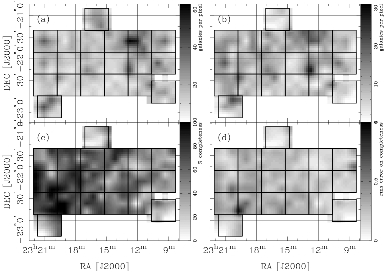
Figure 11.— Bright completeness maps. Panel (a) shows the total surface density of galaxies in the target area with R$\leq 18.5$ counted in 10.9$\arcmin$ pixels. Panel (b) shows the surface density of bright galaxies with redshift measurements $Q\geq 3$. Panel (c) shows the redshift completeness. Panel (d) shows the rms uncertainty on the completeness estimates.

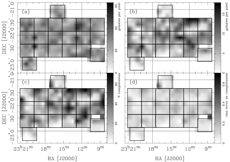
Figure 12.— Identical to Fig. 11, but for the galaxies with $18.5<$R$\leq 19.5$.

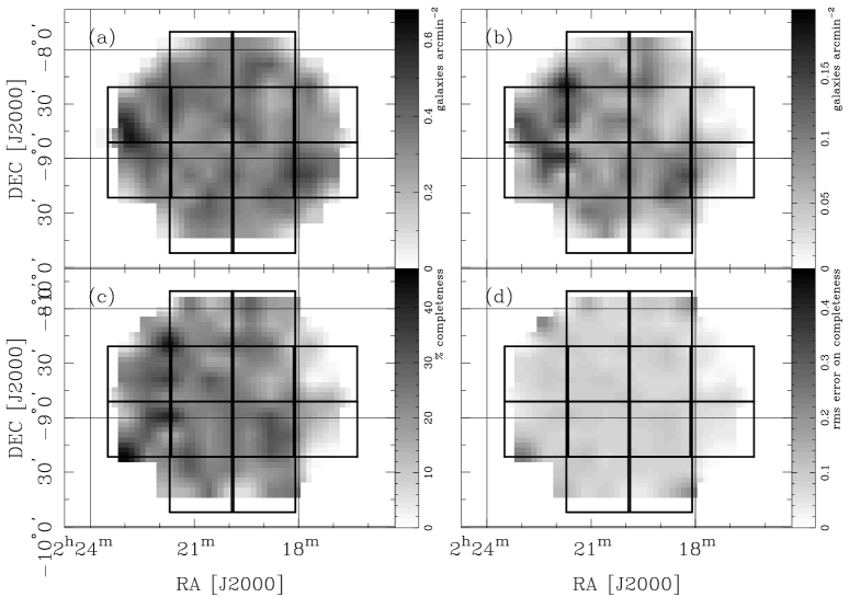
Figure 13.— Cetus region completeness masks for the bright galaxy catalogue: $R>18.5$. Individual panels are identical to those of Fig. 11.

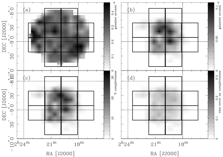
Figure 14.— Cetus field region completeness masks for the faint galaxy catalogue: $18.5<$R$\leq 19.5$. Individual panels are identical to those of Fig. 11.

5. Cluster Detection

We now identify clusters and large groups in the Aquarius and Cetus regions from the redshift data. In addition to our 2723 ($Q\geq 3$) 2dF redshifts for Aquarius, we also used 31 redshifts taken from the NED archives for this analysis. Possible duplicates were rejected by requiring that any galaxy with a NED redshift should be separated by $>5\arcsec$ from any galaxy in our 2dF redshift catalog. These literature redshifts were included in the survey completeness estimates described above.

The cluster candidates were identified as follows: First, we generated smoothed images of the galaxy distribution. This was done for a series of redshift planes running from $z_{\rm p}=0$ to $z_{\rm p}=0.42$, separated by $\Delta(cz)=1000\,{\rm km\,s}^{-1}$. In generating these maps each galaxy was weighted by the inverse of the local survey completeness and Gaussian weighted (with $\sigma=1000\,{\rm km\,s}^{-1}$) according to its difference in radial velocity from the redshift plane. These frames were all of size $832\times 832$ pixels with pixel scale $14.875\arcsec/{\rm pixel}$. These were then smoothed in the angular direction with a 2D Gaussian of scale $33\arcsec/z_{\rm p}$. For the nearest cluster in our catalogue, $z\sim 0.06$, this corresponded to a physical smoothing scale of $\sim 450$ kpc $h^{-1}$ and for the most distant cluster at $z\sim 0.3$, a scale of $\sim 350$ kpc $h^{-1}$.

Next, we located the peaks in the smoothed frames. This was done using the peak finder algorithm in the IMCAT software package (Kaiser, Squires & Broadhurst 1995). In accord with the image generation, we detected peaks using a Gaussian smoothing filter with a radius of $33\arcsec/z_{\rm p}$. The peak detection threshold was set to be a low significance threshold $\nu=2$. A “galaxy flux” was then associated to each of the identified peaks, by summing over all pixels within $33\arcsec/z_{\rm p}$ from the central pixel. All peaks below a flux threshold of 375 galaxies were rejected. This cutoff level was arrived at by determining the highest peak height that would allow us to recover all of the previously known clusters in the fields. In practice, our detection scheme would typically recover the same structure in several adjacent redshift planes. We rejected such duplicates, by identifying those peaks that had a corresponding peak with higher flux in a neighbouring plane and that were separated by less than one Abell radius $R_{A}=1\arcmin 7/z$.

As a first approximation, the redshift of each candidate cluster was assumed to be that of the plane $z_{\rm p}$. We then defined as cluster members all galaxies within a radial velocity interval of width $\Delta(cz)=6000\,{\rm km\,s}^{-1}$, centered on the estimated cluster redshift. Finally, we generated a cluster catalog containing clusters that had $N\geq 9$ members with spectroscopically measured redshifts. This selection criterion was motivated by the desire to have enough redshifts to make at least a rough estimate of the cluster velocity dispersion (see the following section). The final cluster catalogs contain a total of 48 identified objects in Aquarius (see Table 1) and 14 clusters in Cetus (see Table 2).

In these Tables, column (1) is the identifier in our catalog, where we have adopted the naming conventions “AQ HHMM.M(+/-)DDMM” for the Aquarius clusters and “CET HHMM.M(+/-)DDMM” for the Cetus clusters. The last nine digits are the celestial coordinates of the objects, which we take to be the position of the peaks in the smoothed galaxy distributions. Here, the right ascension is given in units of hours and minutes, with one decimal, and the declination is given in units of degrees and arc-minutes. The precision of these coordinates may vary significantly for different clusters because of variations in survey completeness as a function of sky position (see Figs 11 – 14). Furthermore, we note that the minimum distance between the 2dF fibres limits our spectroscopic sampling in the densest parts of the clusters, and this limits the precision of positional estimates based on our spectroscopic data only. Such sampling restrictions will also limit the detection efficiency for the more distant clusters, which cover a smaller sky area. An updated catalog with more accurate coordinates for the center of each cluster will be reported in a future paper, based on our $B$- and $R$-band imaging data from the ESO WFI.

5.1. Aquarius Region

In column (2) of Table 1 we give the ACO cluster catalog name or if the cluster does not have an ACO identifier, then we give the AqrCC catalog name (Caretta02). Of the 23 previously known clusters in our Aquarius survey region, we are able to robustly identify 20, of which five had previously unknown redshifts and two appear to be multiple systems. In addition to these, two previously known clusters (A2541 (catalog ) and A2550 (catalog )) are recovered by our detection method when we include 58 literature redshifts for galaxies that are just outside our survey region and that are fainter than $R=19.5$ (see next section for details). The only previously known system that we fail to detect is the cluster candidate AqrCC 43 (catalog ), which is a peak in the 2D galaxy distribution on the sky (Caretta02), located close to the Northern edge of our survey region.

Table 1 also contains data for 26 additional clusters that are previously unknown systems. Figure 15 shows radial velocity histograms for the 48 clusters identified with the methods described here. Figure 16 shows the cluster distribution in Aquarius projected on the sky. Each cluster is represented by a circle, where the scale of the circle is proportional to the Abell radius for the cluster.

Table 1Cluster Redshifts and Velocity Dispersions for the Aquarius Region

ID	other ID	$N$	$z$	$N_{\rm lit}$	$z_{\rm lit}$	$\sigma_{P}$ (${\rm km}\,{\rm s}^{-1}$)	Asym. index	Tail index
(1)	(2)	(3)	(4)	(5)	(6)	(7)	(8)	(9)
AQ2308.5-2124 (catalog )	$\cdots$	12	$0.0847^{+0.0005}_{-0.0006}$	$\cdots$	$\cdots$	$520^{+90}_{-46}$	-0.212	0.705
AQ2308.7-2209 (catalog )	$\cdots$	9	$0.1993^{+0.0003}_{-0.0005}$	$\cdots$	$\cdots$	$382^{+816}_{-160}$	-0.007	1.281
AQ2308.8-2133 (catalog )	A2539 (catalog )	13	$0.1782^{+0.0014}_{-0.0011}$	4	0.1863	$1383^{+317}_{-117}$	-0.522	0.980
AQ2308.8-2214 (catalog )	$\cdots$	16	$0.1361^{+0.0005}_{-0.0007}$	$\cdots$	$\cdots$	$614^{+150}_{-81}$	-0.207	1.054
AQ2309.6-2210 (catalog )	A2540 (catalog )	38	$0.1340^{+0.0006}_{-0.0006}$	8	0.129	$978^{+120}_{-77}$	-0.643	0.800
AQ2309.9-2132 (catalog )	AqrCC 24 (catalog )	25	$0.1097^{+0.0006}_{-0.0004}$	7	0.1109	$701^{+156}_{-84}$	0.902	1.114
AQ2310.5-2155 (catalog )	$\cdots$	18	$0.1107^{+0.0003}_{-0.0002}$	$\cdots$	$\cdots$	$389^{+298}_{-101}$	0.024	1.522
AQ2310.6-2238 (catalog )	A2546 (catalog )	38	$0.1136^{+0.0006}_{-0.0005}$	22	0.113	$901^{+88}_{-70}$	-0.992	0.955
AQ2311.1-2134 (catalog )	$\cdots$	12	$0.1515^{+0.0006}_{-0.0012}$	$\cdots$	$\cdots$	$770^{+795}_{-180}$	-1.102	1.339
AQ2311.1-2135 (catalog )	$\cdots$	14	$0.0903^{+0.0010}_{-0.0009}$	$\cdots$	$\cdots$	$957^{+388}_{-136}$	0.856	0.777
AQ2311.4-2126 (catalog )	AqrCC 32a (catalog )	19	$0.1647^{+0.0007}_{-0.0004}$	$\cdots$	$\cdots$	$912^{+613}_{-293}$	-0.215	2.271
AQ2311.4-2134 (catalog )	AqrCC 32b (catalog )	11	$0.1520^{+0.0006}_{-0.0010}$	$\cdots$	$\cdots$	$621^{+647}_{-231}$	0.171	1.686
AQ2311.8-2158 (catalog )	$\cdots$	18	$0.1545^{+0.0006}_{-0.0005}$	$\cdots$	$\cdots$	$562^{+343}_{-165}$	0.783	1.574
AQ2312.2-2129 (catalog )	A2554 (catalog )	71	$0.1106^{+0.0003}_{-0.0003}$	35	0.1108	$680^{+68}_{-43}$	0.297	1.074
AQ2312.3-2202 (catalog )	$\cdots$	15	$0.1601^{+0.0007}_{-0.0012}$	$\cdots$	$\cdots$	$1123^{+238}_{-176}$	0.319	1.125
AQ2312.5-2205 (catalog )	$\cdots$	12	$0.0891^{+0.0004}_{-0.0010}$	$\cdots$	$\cdots$	$820^{+325}_{-216}$	0.431	1.627
AQ2312.6-2248 (catalog )	AqrCC 34 (catalog )	11	$0.1990^{+0.0004}_{-0.0004}$	$\cdots$	$\cdots$	$374^{+301}_{-83}$	-0.758	1.408
AQ2312.8-2209 (catalog )	$\cdots$	30	$0.1397^{+0.0003}_{-0.0003}$	$\cdots$	$\cdots$	$507^{+91}_{-50}$	-1.088	0.956
AQ2312.8-2213 (catalog )	A2555 (catalog )	23	$0.1109^{+0.0002}_{-0.0002}$	11	0.1106	$366^{+120}_{-99}$	0.172	1.628
AQ2313.1-2135 (catalog )	A2556 (catalog )	46	$0.0881^{+0.0004}_{-0.0004}$	9	0.0871	$816^{+137}_{-99}$	0.068	1.434
AQ2314.1-2145 (catalog )	$\cdots$	9	$0.3047^{+0.0009}_{-0.0002}$	$\cdots$	$\cdots$	$447^{+314}_{-333}$	0.736	1.065
AQ2314.2-2241 (catalog )	$\cdots$	9	$0.1306^{+0.0005}_{-0.0004}$	$\cdots$	$\cdots$	$288^{+1111}_{-71}$	-0.198	3.138
AQ2314.5-2118 (catalog )	$\cdots$	17	$0.1495^{+0.0007}_{-0.0007}$	$\cdots$	$\cdots$	$1048^{+463}_{-239}$	-0.081	1.412
AQ2314.8-2119 (catalog )	A2565 (catalog )	16	$0.0845^{+0.0006}_{-0.0005}$	12	0.0825	$584^{+114}_{-63}$	1.155	1.130
AQ2315.0-2223 (catalog )	$\cdots$	14	$0.0857^{+0.0012}_{-0.0017}$	$\cdots$	$\cdots$	$1077^{+228}_{-74}$	1.160	0.728
AQ2315.1-2149 (catalog )	$\cdots$	16	$0.0873^{+0.0003}_{-0.0003}$	$\cdots$	$\cdots$	$478^{+313}_{-306}$	-0.180	1.083
AQ2315.7-2138 (catalog )	$\cdots$	9	$0.1253^{+0.0004}_{-0.0003}$	$\cdots$	$\cdots$	$309^{+381}_{-67}$	-0.697	2.161
AQ2316.4-2143 (catalog )	$\cdots$	9	$0.0620^{+0.0008}_{-0.0025}$	$\cdots$	$\cdots$	$1016^{+1017}_{-553}$	0.039	1.655
AQ2316.8-2233 (catalog )	$\cdots$	10	$0.0995^{+0.0007}_{-0.0010}$	$\cdots$	$\cdots$	$826^{+630}_{-323}$	1.107	1.577
AQ2317.2-2212 (catalog )	A2568 (catalog )	16	$0.1383^{+0.0005}_{-0.0005}$	6	0.1397	$488^{+75}_{-41}$	-0.443	0.724
AQ2317.3-2213 (catalog )	$\cdots$	15	$0.0643^{+0.0002}_{-0.0002}$	$\cdots$	$\cdots$	$152^{+187}_{-24}$	-1.126	3.054
AQ2317.4-2223 (catalog )	AqrCC 48a (catalog )	15	$0.0874^{+0.0009}_{-0.0008}$	5	0.0827	$654^{+401}_{-143}$	-1.484	1.178
AQ2317.9-2152 (catalog )	$\cdots$	10	$0.1405^{+0.0006}_{-0.0002}$	$\cdots$	$\cdots$	$314^{+182}_{-139}$	1.341	1.222
AQ2318.1-2135 (catalog )	$\cdots$	9	$0.1209^{+0.0013}_{-0.0009}$	$\cdots$	$\cdots$	$1202^{+743}_{-343}$	0.257	2.025
AQ2318.6-2135 (catalog )	$\cdots$	15	$0.1115^{+0.0032}_{-0.0009}$	$\cdots$	$\cdots$	$1586^{+511}_{-261}$	0.070	0.678
AQ2318.9-2232 (catalog )	AqrCC 48b (catalog )	14	$0.0894^{+0.0003}_{-0.0007}$	5	0.0827	$417^{+261}_{-126}$	-0.851	0.940
AQ2319.7-2140 (catalog )	AqrCC 56 (catalog )	23	$0.0849^{+0.0003}_{-0.0003}$	$\cdots$	$\cdots$	$340^{+46}_{-32}$	-0.490	0.755
AQ2319.8-2203 (catalog )	A2575 (catalog )	16	$0.2731^{+0.0011}_{-0.0010}$	$\cdots$	$\cdots$	$1200^{+243}_{-155}$	0.016	1.134
AQ2319.8-2227 (catalog )	A2576 (catalog )	29	$0.1895^{+0.0006}_{-0.0006}$	9	0.1876	$887^{+131}_{-87}$	0.048	1.047
AQ2320.1-2238 (catalog )	$\cdots$	9	$0.1235^{+0.0004}_{-0.0005}$	$\cdots$	$\cdots$	$305^{+115}_{-25}$	0.440	0.854
AQ2320.8-2255 (catalog )	$\cdots$	10	$0.1496^{+0.0003}_{-0.0002}$	$\cdots$	$\cdots$	$182^{+1162}_{-41}$	1.048	0.610
AQ2320.8-2304 (catalog )	A2577 (catalog )	11	$0.1256^{+0.0006}_{-0.0009}$	7	0.1248	$496^{+252}_{-59}$	-0.584	1.222
AQ2320.8-2308 (catalog )	A2580 (catalog )	18	$0.0890^{+0.0009}_{-0.0010}$	17	0.0890	$1013^{+370}_{-151}$	-0.909	1.058
AQ2321.1-2128 (catalog )	$\cdots$	9	$0.1410^{+0.0002}_{-0.0004}$	$\cdots$	$\cdots$	$264^{+554}_{-73}$	0.599	3.069
AQ2321.3-2135 (catalog )	A2579 (catalog )	30	$0.1103^{+0.0004}_{-0.0004}$	9	0.1114	$543^{+98}_{-61}$	-0.706	1.110
AQ2321.3-2224 (catalog )	AqrCC 62 (catalog )	9	$0.1935^{+0.0004}_{-0.0005}$	$\cdots$	$\cdots$	$417^{+138}_{-80}$	0.010	1.359
AQ2321.7-2147 (catalog )	$\cdots$	17	$0.1233^{+0.0003}_{-0.0003}$	$\cdots$	$\cdots$	$416^{+648}_{-129}$	-0.085	2.382
AQ2322.1-2205 (catalog )	A3996 (catalog )	17	$0.1125^{+0.0003}_{-0.0011}$	6	0.0854	$841^{+918}_{-486}$	-0.625	1.634

Note. — See the text for further comments on specific clusters.

Figure 15.— Velocity histograms for the 48 clusters identified in the Aquarius region. The properties of each cluster are listed in Table 1

Figure 16.— 2D plot of the distribution of the identified clusters in the Aquarius region (left panel: Clusters with $z<0.12$; right panel: Clusters with $z>0.12$). The member galaxies for all clusters with $N\geq 9$ spectroscopically determined galaxy redshifts are indicated by the asterisks, and the Abell radius $R_{A}$ of each cluster is indicated by the circles.

5.2. Cetus Region

In the typical field region in Cetus, our cluster detection method recovers 12 new galaxy clusters in addition to the 2 previously known clusters identified in column (2) of Table 2. Figure 17 shows radial velocity histograms for all 14 clusters. Figure 18 shows the cluster distribution projected on the sky. Each cluster is represented by a circle, where the scale of the circle is proportional to the Abell radius for the cluster.

6. Cluster Redshifts and Velocity Dispersions

We now present estimates of the centroid redshifts and the velocity dispersions for the cluster candidates. Owing to the modest number of observed galaxies per cluster, typically between 9 and 71, it was important to use robust statistical estimators to avoid problems caused by e.g., deviations from a Gaussian velocity distribution and contamination from fore- and background galaxies. We therefore use the biweight estimators of location and scale described by Beers et al. (1990), to measure velocity dispersions and centroid redshifts. Confidence intervals for the estimates were calculated using the bias corrected and accelerated bootstrap method (Efron 1987) with 10,000 bootstrap replications. These robust estimators and methods for determining confidence intervals have been well tested on redshift samples like ours (see e.g., Beers et al. 1990; Girardi et al. 1993; Borgani et al. 1999; Irgens et al. 2002). Our statistical analysis was performed using the ROSTAT program kindly provided by Dr. T. C. Beers.

The cluster redshifts and one-dimensional velocity dispersion estimates, together with 68% confidence limits, are presented for the Aquarius region in Table 1 as columns (4) and (7) and for the Cetus region in Table 2 as columns (4) and (6). Figures 8 and 9 show the cluster candidates overlayed on the measured galaxy distribution.

Column (3) in both tables shows the number of galaxy redshifts used in these estimates for each cluster. We note that from the sample, there are 15 clusters for which estimates were derived from only 9 redshifts, and as expected these have respectively large confidence limits for the velocity dispersion estimates. Previous redshift estimates have been made by Caretta02 for a total of 15 clusters in our Aquarius survey region (one of which we identify as a double system). These values are listed in column (6) of Table 1, and the number of cluster members used for their redshift estimate is given in column (5). We find very good agreement with the literature redshifts for 12 clusters, while 3 clusters have discrepant redshift values. These cases are discussed in detail below. However, we point out that our estimates are based upon more (in most cases many more) galaxies than Caretta02. In the Cetus region, Romer et al. (2000) have published a redshift for a single cluster, listed in column (5) of Table 2, which is consistent with our value.

Columns (8) and (9) of Table 1 and columns (7) and (8) of Table 2 show the asymmetry index and normalized tail index defined by Bird & Beers (1993). For a Gaussian distribution, the asymmetry index is zero and the normalized tail index is unity. Large deviations from these numbers are a strong indication that the cluster is not in dynamic equilibrium, or that it is strongly contaminated by non-cluster galaxies, i.e., that the found velocity dispersion is not to be taken as a good measurement of its dynamical mass. For our sample sizes, an asymmetry index with absolute value larger than 0.9 and/or a reduced tail index larger than 1.5 (somewhat higher values for the clusters with $N<25$) should signify that the cluster velocity dispersion is suspect. We see that the bootstrap method gives large confidence limits on the velocity dispersions for these clusters.

Table 2Cluster Redshifts and Velocity Dispersions for the Cetus Region

ID	other ID	$N$	$z$	$z_{\rm lit}$	$\sigma_{P}$ (${\rm km}\,{\rm s}^{-1}$)	Asym. index	Tail index
(1)	(2)	(3)	(4)	(5)	(6)	(7)	(8)
CET0218.0-0859 (catalog )	A339	12	$0.1123^{+0.0011}_{-0.0012}$	$\cdots$	$778^{+179}_{-82}$	0.436	0.735
CET0218.9-0848 (catalog )	$\cdots$	9	$0.0745^{+0.0002}_{-0.0001}$	$\cdots$	$118^{+1065}_{-41}$	-0.843	0.650
CET0219.3-0814 (catalog )	$\cdots$	25	$0.1097^{+0.0002}_{-0.0002}$	$\cdots$	$342^{+112}_{-79}$	-0.317	2.026
CET0219.3-0935 (catalog )	$\cdots$	9	$0.0551^{+0.0004}_{-0.0006}$	$\cdots$	$437^{+886}_{-381}$	0.710	2.313
CET0220.7-0838 (catalog )	$\cdots$	26	$0.1102^{+0.0004}_{-0.0004}$	$\cdots$	$697^{+236}_{-146}$	0.277	1.375
CET0221.2-0926 (catalog )	$\cdots$	20	$0.1609^{+0.0005}_{-0.0005}$	$\cdots$	$526^{+72}_{-41}$	-0.034	0.738
CET0221.6-0809 (catalog )	$\cdots$	9	$0.1056^{+0.0026}_{-0.0040}$	$\cdots$	$1484^{+542}_{-115}$	-0.205	0.811
CET0221.5-0827 (catalog )	$\cdots$	10	$0.2302^{+0.0002}_{-0.0003}$	$\cdots$	$251^{+74}_{-45}$	0.179	1.307
CET0222.0-0840 (catalog )	$\cdots$	24	$0.1097^{+0.0005}_{-0.0003}$	$\cdots$	$589^{+404}_{-133}$	1.028	1.584
CET0222.4-0821 (catalog )	$\cdots$	9	$0.2152^{+0.0006}_{-0.0007}$	$\cdots$	$569^{+149}_{-39}$	-1.223	0.718
CET0222.4-0856 (catalog )	$\cdots$	9	$0.1668^{+0.0002}_{-0.0001}$	$\cdots$	$165^{+283}_{-56}$	-1.435	3.144
CET0222.7-0858 (catalog )	$\cdots$	12	$0.2234^{+0.0012}_{-0.0011}$	$\cdots$	$780^{+210}_{-83}$	-0.487	0.489
CET0223.0-0912 (catalog )	$\cdots$	9	$0.1598^{+0.0008}_{-0.0028}$	$\cdots$	$918^{+567}_{-266}$	-1.023	-0.907
CET0223.3-0851 (catalog )	RX J0223.4-0852	19	$0.1615^{+0.0007}_{-0.0014}$	0.163	$1035^{+220}_{-170}$	-0.705	0.874

Figure 17.— Velocity histograms for the 14 clusters identified in the Cetus region. The properties of each cluster are listed in Table 2

Figure 18.— 2D plot of the distribution of the identified clusters in the Cetus region. The member galaxies for all clusters with $N\geq 9$ spectroscopically determined galaxy redshifts are indicated by the asterisks, and the Abell radius $R_{A}$ of each cluster is indicated by the circles.

We have made some notes on specific clusters:

A2539

Caretta02 report that this cluster appears to be a superposition of groups at $z\sim 0.175$ and $z\sim 0.186$. Our redshift estimate falls between these two values, but is more consistent with the lower value. The rather high estimated velocity dispersion could be caused by such a superposition of two groups along the line of sight, although the asymmetry index and the normalized tail index do not indicate a significant departure from a Gaussian distribution.

A2540

Our redshift value of $z=0.134$ is significantly higher than the value of $z=0.129$ measured by Caretta02. However, our estimate is based on a significantly larger number of redshifts.

A2546

This appears to form a double system with nearby A2541 (catalog ), which is located near the Southeastern end of our survey region. By including additional literature redshifts of galaxies located slightly outside our survey region, we measure a redshift $z=0.1124^{+0.0014}_{-0.0011}$ and velocity dispersion of $995^{+854}_{-423}\,{\rm km\,s}^{-1}$, based on 11 member galaxies. This redshift value is consistent with the redshift reported by Caretta02 ($z=0.1135$, based on 16 galaxies).

AQ2311.4-2126

The coordinates of the cluster candidate AqrCC 32 (catalog ) identified by Caretta02 places it between our clusters AQ2311.4-2126 (catalog ) and AQ2311.4-2134 (catalog ), and it is most likely a superposition of these two clusters.

A2550

While this cluster was not recovered using our standard detection scheme outlined in § 5, a significant peak was detected at this location when using all available literature redshifts in the region. We note that the apparent center of this cluster is located in a region where the completeness of our spectroscopic survey is particularly low (see Figs. 11 and 12). Our measured redshift value $z=0.1151^{+0.0022}_{-0.0013}$, based on 14 galaxies, is discrepant from previously reported estimates: Caretta02 give a value $z=0.1226$ from 6 galaxies, while Kowalski, Ulmer & Cruddace (1983) reported $z=0.1543$ based on a single redshift measurement. The latter value is close to the redshifts of the clusters AQ2311.4-2136 (catalog ) and AQ2311.4-2134 (catalog ) which are both located within $\sim 0.5\arcdeg$ from the ACO position of A2550 (catalog ). On inspection of a deep $R$-band image of this field, from our ESO WFI data (Dahle et al. 2004; in preparation), we find that the bright elliptical galaxy 2MASX J23113576-2144462 (catalog ) is dominating the center of A2550 (catalog ). Its redshift was measured as $z=0.1216$ by Batuski et al. (1999), similar to the cluster redshift value reported by Caretta02. Furthermore, we note that line-of-sight contamination from the very rich nearby cluster A2554 (catalog ) may have influenced our results, and the high velocity dispersion ($1427^{+410}_{-210}\,{\rm km\,s}^{-1}$) and asymmetry index (1.4) of our galaxy sample indicates that we may be probing a filamentary structure linked to A2554 (catalog ) rather than A2550 (catalog ).

A2554

Based on 23 cluster members, Colless & Hewett (1987) measured a velocity dispersion of $797^{+165}_{-114}$  km  s^-1, consistent with our estimate at the $1\sigma$ level.

A2565

Our redshift value is slightly discrepant from that reported by Caretta02, but our cluster position is also significantly mis-aligned with their position. We note that this cluster is located in a region where the spectroscopic completeness value is particularly low, and our position is shifted in a direction towards a region where the completeness is higher. Thus, we are probably sampling a slightly different region than Caretta02, and the high asymmetry index indicates that our redshift estimate may be significantly affected by filaments or other structures outside the virial radius of the cluster.

AQ2317.4-2223

The coordinates of the cluster candidate AqrCC 48 (catalog ), described by Caretta02 as “a superposition of small groups”, places it between our clusters AQ2317.4-2223 (catalog ) and AQ2318.9-2232 (catalog ), and it is most likely a superposition of these two objects.

A2576

Batuski et al. (1995) reported a velocity dispersion measurement of $630$  km  s^-1 for this cluster, which is somewhat lower than the value we measure. However, their measurement is based on only 10 member galaxies, so the uncertainty should be significantly higher than for our measurement.

AQ2321.3-2224

This cluster probably corresponds to the cluster candidate AqrCC 62 (catalog ) reported by Caretta02. While these authors did not detect a concentration in redshift space at this location, we find from our data a corresponding galaxy group (or poor cluster) at $z\sim 0.193$.

A3996

While the redshift measurement of Caretta02 ($z=0.0854$) is significantly lower than our value, these authors report A3996 (catalog ) to be a superposition of small groups. Our redshift value is quite similar to that reported by Batuski et al. (1999) ($z=0.1155$), based on 8 redshifts. The high tail index and highly uncertain velocity dispersion indicate that this cluster may be significantly affected by foreground/background contamination.

7. The Aquarius Superclusters

Based on a percolation analysis of Abell and ACO clusters in Aquarius, Batuski et al. (1999) interpreted the region at $0.08<z<0.12$ as a single supercluster structure. In contrast, Caretta02 found that the Aquarius region contains two separate superclusters, seen in projection, at $z\sim 0.08$ and $z\sim 0.11$. While Batuski et al. (1999) argued that these two superclusters are physically linked and form a single system, most of the evidence for this link came from an erroneous redshift for A2541 (catalog ). In fact, this cluster is situated within the densest portion of the most distant of the two superclusters rather than in a region between the superclusters. The cone plot of Fig. 8, clearly shows strong clustering at $z\sim 0.08$ and $z\sim 0.11$, separated by a region of comparatively low density.

The overdensities and total masses of these structures can be estimated from the measured galaxy velocity dispersions of their member clusters. A lower limit on the supercluster mass can be found by summing the estimated masses of all the clusters within their respective virial radii, and an upper limit can be found by assuming a given cluster density profile and integrating this for all clusters over the volume covered by the supercluster.

We assume that the clusters generally follow the density profile of cold dark matter halos proposed by Navarro, Frenk, & White (1997, hereafter NFW). While this model has been shown to provide a good fit to the radial cluster density profile in the virialized region of clusters (Arabadjis, Bautz, & Garmire 2002; Biviano & Girardi 2003; Dahle, Hannestad, & Sommer-Larsen 2003b), there are currently only limited constraints on the density profile in the infall region beyond the virial radius (Rines et al. 2003; Kneib et al. 2003). Also, clusters embedded in the rare, high-density environment of a supercluster may have density profiles that deviate significantly from those of average clusters. With our weak lensing data set from WFI imaging, we will be able to directly constrain the density profiles of clusters within the superclusters and provide more accurate estimates of the supercluster masses. Our density estimates given below do not take into account any redshift space distortions due to departures from the Hubble flow. In reality, the cluster distribution could be either flattened or elongated in the $z$ direction by cluster peculiar velocities.

For each cluster, we assume an NFW model with an effective velocity dispersion $\sigma_{v}=\sqrt{50}H(z)r_{200}$, where $H(z)$ is the Hubble parameter, and $r_{200}$ is the radius within which the average mass density is 200 times the critical density at the relevant redshift. The average mass within $r_{200}$ of the members of the superclusters discussed below is $\langle M_{200}\rangle\sim 4\times 10^{14}h^{-1}M_{\sun}$. For this cluster mass, an NFW cluster in a $\Lambda$CDM universe has a predicted concentration parameter $C=6$, which we will adopt as a general value. In a $\Lambda$CDM universe, the virial radius is actually slightly larger than $r_{200}$, while the two are the same in an Einstein-de Sitter universe.

7.1. The $z\sim 0.11$ Supercluster

As noted in § 2, Batuski et al. (1999) identified a particularly dense knot of five $R\geq 1$ ACO clusters contained within a sphere of radius 10 $h^{-1}$ Mpc at $z=0.11$, representing a spatial number density 150 times the mean density of $R\geq 1$ ACO clusters. By this measure, the Aquarius knot represents the strongest overdensity of any known supercluster. The knot is very obvious in Figure 8, and corresponds to the densest part of the supercluster.

All of the 5 ACO clusters forming the knot noted by Batuski et al. (1999) are located within our survey field. In § 6 (see the note regarding A2546 (catalog )) we provide a new redshift estimate for another $R\geq 1$ ACO cluster, A2541 (catalog ), which makes it a sixth member of the knot. In addition, we find that AqrCC 24 (catalog ) plus two previously unknown systems are also members of the knot at $z=0.11$.

The lower limit on the supercluster mass obtained from the sum of the $M_{200}$ values of the nine clusters within our survey region is $4.5\times 10^{15}h^{-1}M_{\sun}$. Integrating NFW density profiles for the nine galaxy clusters over the volume bounded by $23^{\rm h}09^{\rm m}00^{\rm s}<\alpha<23^{\rm h}22^{\rm m}30^{\rm s}$, $-23\arcdeg 10\arcmin<\delta<-21\arcdeg 15\arcmin$ and $0.109<z<0.114$, corresponding to a volume of $17\times 8.5\times 15h^{-3}{\rm Mpc}^{3}$, gives an estimate of the total mass of $8.3\times 10^{16}h^{-1}M_{\sun}$. The lower and upper limits for the mass correspond to overdensities of $\rho=17\bar{\rho}$ and $\rho=330\bar{\rho}$ within this volume.

7.2. The $z\sim 0.08$ supercluster

We identify 11 clusters and groups in the most nearby Aquarius supercluster at $0.084<z<0.091$, of which three are ACO clusters, three more were detected by Caretta02 (AqrCC 48 (catalog ), which we interpret to be a binary system, and AqrCC 56 (catalog )), and the remaining five are new detections. The sum of their $M_{200}$ masses is $3.2\times 10^{15}h^{-1}M_{\sun}$, and their integrated masses over a volume of $15\times 7.9\times 20h^{-3}{\rm Mpc}^{3}$ (bounded by $23^{\rm h}08^{\rm m}00^{\rm s}<\alpha<23^{\rm h}22^{\rm m}30^{\rm s}$, $-22\arcdeg 55\arcmin<\delta<-21\arcdeg 15\arcmin$ and $0.084<z<0.091$) is $8.3\times 10^{16}h^{-1}M_{\sun}$. The lower and upper limits for the mass correspond to overdensities of $\rho=13\bar{\rho}$ and $\rho=330\bar{\rho}$ within this volume. We note that our Aquarius survey field is too small to encompass the entire supercluster, and Caretta02 identify several supercluster members outside our field.

The integrated masses of the $z=0.11$ and $z=0.08$ structures are similar to the upper limit on the mass of the Corona Borealis supercluster ($M<8\times 10^{16}h^{-1}M_{\sun}$) estimated by Small et al. (1998).

8. Summary

In this paper we have presented a spectroscopic analysis of $\sim 4000$ galaxies down to $R<19.5$ in the direction of Aquarius and Cetus. These observations form part of our wider efforts to conduct a spectro-photometric and weak lensing survey of these two regions. The spectroscopic data are sensitive to structures out to $\sim$1 Gpc or equivalently $z\sim 0.4$. These data will greatly aid our ongoing efforts to measure the dark matter distribution in these regions and quantify the bias over a large range of scales and environments.

We described the survey that we are conducting, focusing on the spectroscopic input catalogue. We then presented our 2dF observations and the reduction of the spectra. We characterized the spectroscopic sample by considering the median spectra, finding evolution of the median galaxy spectrum with redshift. This evolution was attributed to selection effects, rather than any true evolution in the galaxy population. We presented spatial diagrams for the two target regions and also quantified the number redshift distributions. These displayed a large amount of structure and were poorly fit by a 2dFGRS-like number redshift distribution. For our future lensing analysis, where these quantities are required, we will use direct fits to the data. Using the full redshift space sample we then identified clusters in both the Aquarius and Cetus regions. In Aquarius we found a total of 48 clusters and galaxy groups, 26 of which had not before been noted, and for 5 of those that had, we provided the first spectroscopic redshift estimates. For Cetus we found 14 clusters and galaxy groups, of which 12 were previously unknown systems. For each candidate system we then provided estimates of the centroid redshift and velocity dispersion. We showed that there are two superclusters in Aquarius, one at redshift $z=0.08$ and the other at $z=0.11$. For these we estimated the overdensities and total masses, finding that they were similar to the Corona Borealis supercluster.

In the future, we intend to characterize the galaxies through their spectral energy distributions using a principal components analysis (Madgwick et al. 2002). This will allow us to explore the putative result that early-type galaxy light is an unbiased tracer of the dark matter (Kaiser et al. 1998; Gray et al. 2002; Dahle et al. 2002). In addition to the primary goals, we anticipate that when fully complete this survey will provide other valuable scientific information. For example, comparison of the weak lensing data with the optically identified clusters and with the archival X-ray data, will allow us to assess the objectivity of optical and X-ray luminosity selection methods for cluster surveys (Dahle et al. 2003a). This will be important to quantify if cluster abundance surveys that aim to constrain cosmological parameters are to be taken seriously in this new age of precision.

References

- Abell (1961) Abell, G. O. 1961, AJ, 66, 607
- Abell, Corwin & Olowin (1989) Abell, G., Corwin, H., & Olowin, R. 1989, ApJS, 70, 1; (ACO)
- Arabadjis, Bautz, & Garmire (2002) Arabadjis, J. S., Bautz, M. W., & Garmire, G. P. 2002, ApJ, 572, 66
- Bacon & Taylor (2003) Bacon, D., & Taylor, A. N., 2003, MNRAS, 344, 1307
- Bailey, Glazebrook & Bridges (2002) Bailey, J., Glazebrook, K., & Bridges, Y. 2002, “The 2dF user manual”, http://www.aao.gov.au/2df/manual.html; (BGB02)
- Batuski et al. (1995) Batuski, D. J., Maurogordato, S., Balkowski, C., & Olowin, R. P. 1995, A&A, 294, 677
- Batuski et al. (1999) Batuski, D. J., Miller, C. J., Slinglend, K. A., Balkowski, C., Maurogordato, S., Cayatte, V., Felenbok, P., & Olowin, R. 1999, ApJ, 520, 491
- Beers et al. (1990) Beers, T. C., Flynn, K., & Gebhardt, K. 1990, AJ, 100, 32
- Benson et al. (2000) Benson, A. J., Cole, S., Frenk, C. S., Baugh, C. M., & Lacey, C. G., 2000, MNRAS, 311, 793
- Bird & Beers (1993) Bird, C. M., & Beers, T. C. 1993, AJ, 105, 1596
- Biviano & Girardi (2003) Biviano, A., & Girardi, M. 2003, ApJ, 585, 205
- Blanton et al. (2003) Blanton, M., & The SDSS Team, 2003, ApJ, 592, 819
- Borgani et al. (1999) Borgani, S., Girardi, M., Carlberg, R. G., Yee, H. K. C., & Ellingson, E. 1999, ApJ, 527, 572
- Caretta et al. (2002) Caretta, C., Maia, M., Kawasaki, W., & Willmer, C. 2002, AJ, 123, 1200; (Caretta02)
- Ciardullo et al. (1985) Ciardullo, R., Ford, H., & Harms, R. 1985, ApJ, 293, 69
- Coleman, Wu & Weedman (1980) Coleman, G. D., Wu, C.-C., & Weedman, D. W. 1980, ApJS, 43, 393
- Colless & Hewett (1987) Colless, M., & Hewett, P. 1987, MNRAS, 224, 453
- Colless et al. (2001) Colless, M., & The 2dFGRS Team, 2001, MNRAS, 328, 1039
- Dahle et al. (2002) Dahle, H., Kaiser, N., Irgens, R., Lilje, P. B., & Maddox, S. 2002, ApJS, 139, 313
- Dahle et al. (2003a) Dahle, H., Pedersen, K., Lilje, P. B., Maddox, S. J., & Kaiser, N. 2003a, ApJ, 591, 662
- Dahle, Hannestad, & Sommer-Larsen (2003b) Dahle, H., Hannestad, S., & Sommer-Larsen, J. 2003b, ApJ, 588, L73
- Efron (1987) Efron, B. 1987, Journal of the American Statistical Association, 82, 171
- Efstathiou & Moody (2001) Efstathiou, G., & Moody, S. 2001, MNRAS, 325, 1603
- Girardi et al. (1993) Girardi, M., Biviano, A., Giuricin, G., Mardirossian, F., & Mezzetti, M. 1993, ApJ, 404, 38
- Gray et al. (2002) Gray, M. E., Taylor, A. N., Meisenheimer, K., Dye, S., Wolf, C., & Thommes, E. 2002, MNRAS, 568, 141
- Hambly et al. (2001a) Hambly, N. C., MacGillivray, H. T., Read, M. A., Tritton, S. B., Thomson, E. B., Kelly, B. D., Morgan, D. H., Smith, R. E., Driver, S. P., Williamson, J., Parker, Q. A., Hawkins, M. R. S., Williams, P. M., & Lawrence, A. 2001a, MNRAS, 326, 1279
- Hambly et al. (2001b) Hambly, N., Irwin, M. J., & MacGillivray, H. T. 2001b, MNRAS, 326, 1315
- Hoekstra et al. (2001) Hoekstra, H., Yee, H. K. C., & Gladders, M. D. 2001, ApJ, 558, L11
- Hoekstra et al. (2002) Hoekstra, H., van Waerbeke, L., Gladders, M. D., Mellier, Y., & Yee, H. K. C. 2001, ApJ, 558, L11
- Irgens et al. (2002) Irgens, R. J., Lilje, P. B., Dahle, H., & Maddox, S. J. 2002, ApJ, 579, 227
- Kaiser (1992) Kaiser, N. 1992. ApJ, 388, 272
- Kaiser & Squires (1993) Kaiser, N., & Squires, G. 1993. ApJ, 404, 441
- Kaiser, Squires & Broadhurst (1995) Kaiser, N., Squires, G., Broadhurst, T. 1995, ApJ, 449, 460
- Kaiser et al. (1998) Kaiser, N., Wilson, G., Luppino, G., Kofman, L., Gioia, I., Metzger, M., & Dahle, H. 1998, astro-ph/9809268
- Kneib et al. (2003) Kneib, J., Hudelot, P., Ellis, R. S., Treu, T., Smith, G. P., Marshall, P., Czoske, O., Smail, I., & Natarajan, P. 2003, ApJ, 598, 804
- Kowalski, Ulmer & Cruddace (1983) Kowalski, M. P., Ulmer, M. P., & Cruddace, R. G. 1983, ApJ, 268, 540
- Madgwick et al. (2002) Madgwick, D., & The 2dFGRS Team, 2002, MNRAS, 333, 133
- Murray et al. (1978) Murray, S. S., Forman, W., Jones, C., & Giacconi, R. 1978, ApJ, 219, L89
- Navarro, Frenk, & White (1997) Navarro, J. F., Frenk, C. S., & White, S. D. M. 1997, ApJ, 490, 493; (NFW)
- Peacock & Smith (2000) Peacock, J. A., Smith, R. E., 2000, MNRAS, 318, 1144
- Percival et al. (2004) Percival, W. J., & The 2dFGRS Team, 2004, MNRAS, submitted (astro-ph/0406513)
- Postman, Geller & Huchra (1986) Postman, M., Geller, M., & Huchra, J. 1986, AJ, 92, 1238
- Raychaudhury (1989) Raychaudhury, S. 1989, Nature, 342, 251
- Rines et al. (2003) Rines, K., Geller, M. J., Kurtz, M. J., & Diaferio, A. 2003, AJ, 126, 2152
- Romer et al. (2000) Romer, A. K., Nichol, R. C., Holden, B. P., Ulmer, M. P., Pildis, R. A., Merrelli, A. J., Adami, C., Burke, D. J., Collins, C. A., Metevier, A. J., Kron, R. G., & Commons, K. 2000, ApJS, 126, 209
- Schlegel, Finkbeiner & Davis (1998) Schlegel, D. J., Finkbeiner, D. P., & Davis, M. 1989, ApJ, 500, 525
- Schneider (1998) Schneider, P. 1998, ApJ, 498, 43
- Small et al. (1998) Small, T. A., Ma, C., Sargent, W. L. W., & Hamilton, D. 1998, ApJ, 492, 45
- Strauss et al. (2002) Strauss, M. A., & The SDSS Team, 2002, AJ, 124, 1810
- Taylor et al. (2004) Taylor, A. N., Bacon, D. J., Gray, M. E., Wolf, C., Meisenheimer, K., Dye, S., Borch, A., Kleinheinrich, M., Kovacs, Z., & Wisotzki, L., 2004, MNRAS, submitted (astro-ph/0402095)
- Tegmark et al. (2004) Tegmark, M., & The SDSS Team, 2004, ApJ, 606, 702
- Tonry & Davis (1979) Tonry, J., & Davis M. 1979, AJ, 84, 1511
- Wang et al. (2000) Wang, L., Caldwell, R. R., Ostriker, J. P., & Steinhardt, P. J. 2000, ApJ, 530, 17
- Willis, Hewett & Warren (2001) Willis, J., Hewett, P., & Warren, S. 2001, MNRAS, 325, 1002