A General Relativistic Model of Light Propagation
in the Gravitational Field of the Solar System: the Static Case

Abstract

We develop here a new approach for the relativistic modeling of the photons moving into a quasi-Minkowskian space-time, where the metric is generated by an arbitrary n-body distribution within an isolated Solar System. Our model is built on the prescriptions of the theory of General Relativity and leaves the choices of the metric, as well as that of the motion of the observer, arbitrary. Adopting a quasi-Minkowskian expression of the metric accurate to order $(v/c)^{2}$, a thorough numerical test campaign is conducted to verify correctness and reliability of the model equations. The test results show that the model behaves according to predictions. Specifically, comparisons to true (simulated) data demonstrate that stellar distances are reconstructed up to the specified level of accuracy. Although the $(v/c)^{2}$ approximation is not always sufficient for its application to future astrometric experiments, which require modeling to $(v/c)^{3}$, this work serves also as a natural test-ground for the higher order model, whose formulation is now close to completion, and will be presented in a forthcoming paper.

1 Introduction

It is known that the light signal carries most of the physical information on the celestial objects and the physical field it passed through (see Kopeikin and Schäfer (1999); Kopeikin and Mashhoon (2002) and references therein). Part of this information, like e.g. the distance to the source and its velocity, can be extracted by means of (classical) astrometric techniques, but at high-level of accuracy, as demonstrated by ESA space mission Hipparcos, relativistic effects cannot be neglected, and this “relativistic astrometry” can be considered part of fundamental physics (for example, astrometric measurements are one of the natural choices to detect possible deviations from General Relativity generated by a scalar field $\phi$ that couples with the metric tensor $g$ to generate gravity (Damour et al., 2002a, b), or they were used for a possible attempt at measuring the speed of gravity (Kopeikin, 2001; Fomalont and Kopeikin, 2003).

The purpose of this paper is to construct a model of the celestial sphere using the prescriptions of the General Theory of Relativity in order to take into account the relativistic effects suffered by light while propagating through the gravitational field of the Solar System. The planned future astrometric experiments set the optimal target accuracy for such models to the micro-arcsecond level. To this level, it was shown that the light propagation will be affected not only by the mass of the Sun and of the other planets but also by their gravitational quadrupole and their translational and rotational motion (Klioner and Kopeikin, 1992; Kopeikin and Mashhoon, 2002). Assuming that the Solar System is isolated and it is the only source of gravity, then the accuracy of $0.1~{}\mu$arcsec is achieved by considering terms of the background metric up to the order of $(v/c)^{3}$; here $c$ is the velocity of light in vacuum and $v$ is an average velocity for energy balance. In the Solar System this is of $\sim 10$ Km sec^-1.

In this sense, the next generation astrometric missions like GAIA, of ESA (Perryman et al., 2001; Perryman, 2003), and SIM, of NASA (Shao, 1998; Marr, 2003), offer a unique opportunity to test our model. On the other hand, the observational error of these satellites will be pushed to the microarcsecond level ($\mu$arcsec) therefore, the need is to implement a model of the celestial sphere and of the observables which is accurate to that order. As a reference, we recall that Hipparcos (of ESA), the only previous example of a global astrometric mission, had an accuracy of 1 milliarcsecond only.

The construction of a general relativistic many-body astrometric model with the required accuracy is expected to be complicated not only by the mathematical structure of the relativistic equations but also by the numerical methods deployed to implement the model into software code. Therefore it is crucial to have an efficient strategy for testing the model. With this goal in mind, we had already developed a relativistic astrometric model taking as background geometry the exact (unperturbed) Schwarzschild solution (de Felice et al., 1998, 2001). That model was used as a basic touchstone for comparison in the construction of our many-body model. Moreover, since a model limited to the $(v/c)^{2}$ order of accuracy is significantly simpler to handle and test, we decided for a full computer implementation of the $(v/c)^{2}$-model, with the intention to use it as test-ground for the higher order extension, which is our ultimate goal.

Finally, it is worth stressing that our aim was not to add to the theory of light propagation, which is well known, but to develop a relativistic astrometric model with a new theoretical approach that treats the light propagation in a curved space-time in such a way that all the possible relativistic perturbations coming from the gravity sources are naturally included in the light-path reconstruction.

In sections 2 and 3, we define the background geometry in a way compatible with our basic physical assumptions. In section 4 we discuss how to handle light propagation through the Solar System and provide the differential equations which enable us to reconstruct the light trajectory from a distant star to the observer. Then, in sections 5 and 6, we define the observables as the measurements coming from a given satellite and link them to the mathematical boundary conditions needed to integrate the light trajectory. Finally, in sections 7 and 8, we present the test campaign used to validate the model.

In what follows, Greek indices run from $0$ to $3$ and Latin indices run from $1$ to $3$.

2 The space-time metric

The space-time structure which underlies the development of relativistic astrometry must mirror the physical and operational reality experienced by the observer.

The basic step of this project is to identify the background geometry. Our first assumption is that the Solar System is isolated; this means that there are no perturbing bodies intervening between the emitting stars and the Solar System boundaries. It is clear that this assumption may not be fully justified since light rays from distant stars may suffer deflections due to microlensing induced by intervening bodies (e.g., as far as the mission GAIA is concerned, we expect nearly 1000 microlensing events along the Galactic disk during 5 years (Dominik and Sahu, 2000)); indeed they could generate systematic errors in the data reduction of the celestial sphere, however, their number is very small as compared to the number of observations ($\geq 10^{9}$). Furthermore, we know that most of the stars are in a binary system and have proper motion which generates an unsteady gravitational field causing a rotation of the celestial reference frame. However, the rotation coefficients have a temporal variation which amounts to 1 $\mu$arcsec every 20 years, a period much longer than the lifetime of all the future space astrometric missions (Sazhin et al., 1998). So we judge that the above cases do not affect the validity of the hypothesis that the Solar System is isolated.

A second assumption is that the Solar System generates a weak gravitational field. We can then adopt a quasi-Minkowskian coordinate system so that the space-time metric can be written as a perturbation of the Minkowski metric $\eta_{\alpha\beta}$, namely:

$$g_{\alpha\beta}=\eta_{\alpha\beta}+h_{\alpha\beta}+O(h^{2})$$ (1)

where the ${h_{\alpha\beta}}^{\prime}s$ describe effects generated by the bodies of the Solar System and are small in the sense that $|h_{\alpha\beta}|\ll 1$, their spatial variations are of the order of $|h_{\alpha\beta}|$ while their time variations are at most of the order $(v/c)|h_{\alpha\beta}|$. Clearly the metric form (1) is preserved under gauge transformations of the order of $h$. The order of magnitude of the correction terms entering the ${h_{\alpha\beta}}^{\prime}s$, is expressed in terms of powers of $(v/c)$. The ${h_{\alpha\beta}}^{\prime}s$ are at least of the order of $(v/c)^{2}$ (Newtonian terms) hence any higher level of accuracy within the model, is fixed by the power of $(v/c)$ larger than two that one likes to include in the analysis.

Having the above considerations in mind, we choose a solution of Einstein’s equations of the type:

$$g_{\alpha\beta}=\eta_{\alpha\beta}+\sum_{a}h^{(a)}_{\alpha\beta}+O(h^{2})$$ (2)

where now the sum is extended to the bodies of the Solar System. In this approximation, the metric tensor (2) has in general a non-vanishing term $g_{0i}=O[(v/c)^{3}]$ and the non-linearity of the gravitational field is confined to terms $O[(v/c)^{4}]$ in $h_{00}$ and $h_{ij}$.

Moreover, in August 2000 the General Assembly of the IAU stated that a solution like (2) has to be adopted to define the reference frames and time scales in the Solar System (Damour et al., 1991; Brumberg and Kopeikin, 1989). At the first Post-Newtonian level of approximation, the metric tensor nearby any planet of the Solar System takes the form:

$$g_{00} = -1+\frac{2W}{c^{2}}-\frac{2W^{2}}{c^{4}}+O(c^{-5})$$ (3)

$$g_{0i} = -\frac{4W_{i}}{c^{3}}+O(c^{-5})$$ (4)

$$g_{ij} = \delta_{ij}\Big{(}1+\frac{2W}{c^{2}}\Big{)}+O(c^{-4})$$ (5)

with $i,j$ = 1, 2, 3.

In the equations above, $W$ represents a generalization of the Newtonian potential and $W_{i}$ is a vector potential describing the dynamical contribution to the background geometry by the relative motion of the gravitating sources as well as by the peculiarities of their extended structures. The same form (3) to (5) is adopted to describe the metric tensor generated by the whole Solar System referring so forth to the Barycentric Celestial Reference System. Assuming the space-time to be asymptotically flat, the potentials $W$ and $W_{i}$ are a sum of integrals containing terms of gravitational mass and mass-current density. Such integrals are taken over the support of each body of the Solar System. It should be stressed here that the linearized form of the metric, in the weak field and slow motion ($v\ll c$) approximation, is the current support for calculating the ephemerides at the Jet Propulsion Laboratory (Soffel, 2000), California Institute of Technology.

A light ray, on its way to the observer from a distant star, first feels the gravitational field of the Solar System as a point like mass centered in its barycenter, then, as it gets closer, it feels the gravitational perturbations of the individual bodies of the System. To the order of $(v/c)^{2}$, the light ray will feel the contributions from the individual mass structures while the effects arising from their relative motion and spin would enter terms of higher order. Since a time derivative adds a factor of the order of $(v/c)$, time derivatives of the metric coefficients generate terms at least of the order of $(v/c)^{3}$. Our third assumption then is that light rays will not feel perturbations of the order O$[(v/c)^{3}]$ so, within each integration of the light trajectories, the Solar System is approximated in our model to a static, non-rotating and non-expanding gravitating system. A natural consequence of this assumption is that, along with time variations of the metric, we shall also neglect mixed metric coefficients of type $h_{0i}$. Furthermore, in calculating the background metric coefficients which affects the light signal at each spatial point of its trajectory, we need not to consider the spatial location of the individual gravitational source at the corresponding retarded time. This does not mean that the positions of the perturbing bodies are considered fixed during the whole integration, but simply that the ephemeris used do not include the retarded time, and that we neglect, to $(v/c)^{2}$, the effects due to their velocities.

3 Setting the geometry of the celestial sphere

Let ($\xi^{i},\xi^{0}\equiv\tau$) be a quasi-Minkowskian coordinate system with respect to which the space-time metric takes form (1); as stated, the choice to consider only terms up to $(v/c)^{2}$ amounts to assume that space-time is static. Hence there exists a time-like Killing vector field $\eta$, say, along which the physical properties of the space-time do not change and therefore uniquely identifies a time direction. Let the coordinate time $\tau$ be a parameter along $\bm{\eta}$ so that $\eta^{\alpha}=\delta^{\alpha}_{0}$. From the Killing equation $\eta_{(\alpha;\beta)}=0$, where semicolon means covariant derivative with respect to the given metric and round brackets mean symmetrization, one easily deduces that the congruence $C_{\bm{\eta}}$ of Killing lines is, to the required order, vorticity-free. In fact, denoting as $P(\eta)^{\alpha}{}_{\beta}=\delta^{\alpha}_{\beta}+\eta^{\alpha}\eta_{\beta}$ the tensor operator which projects orthogonally to $\bm{\eta}$, one finds:

$$\omega_{\alpha\beta}=P(\eta)^{\rho}{}_{[\alpha}P(\eta)^{\sigma}{}_{\beta]}\eta_{\rho;\sigma}=O[(v/c)^{3}]$$ (6)

where $\omega_{\alpha\beta}$ is the vorticity tensor and square brackets mean anti-symmetrization. A space-time which admits a vorticity-free congruence of lines can be foliated, namely it admits a family of three-dimensional space-like hypersurfaces $S(\xi^{i},\tau)$ which are everywhere orthogonal to $C_{\bm{\eta}}$. It is always possible to choose a coordinate system such that the surfaces $S(\xi^{i},\tau)$ have equation $\tau=$constant; in this case the spatial coordinates can be fixed within each slice up to spatial transformations only. We shall term these surfaces $S(\tau)$.

Let us now consider the unit vector field $\bm{u}$ which is everywhere proportional to $\bm{\eta}$, namely $u^{\alpha}={\rm e}^{\psi}\delta^{\alpha}_{0}$ where $\rm{e}^{\psi}=(-g_{00})^{-1/2}$ is the normalization factor which assures that $u_{\alpha}u^{\alpha}=-1$; the associated one-form has components $u_{\alpha}=-{\rm e}^{-\psi}\frac{\partial\tau}{\partial\xi^{\alpha}}$ so it is proportional to the gradient of $S(\tau)$, as expected. Through each point of a slice $S(\tau)$, for any $\tau$, there goes a time-like curve, orthogonal to $S(\tau)$ and having as tangent a vector of the vector field ${\bf u}$; the totality of these curves through all the points of $S(\tau)$ form a non-intersecting family of curves, or a congruence $C_{\bf u}$, which identifies a physical observer. The property of this observer is to be static with respect to the selected coordinate representation, that is the spatial coordinates do not vary along its world-lines. The parameter $\sigma$ on the congruence, such that $u^{\alpha}=d\xi^{\alpha}/d\sigma$, is the proper-time of the observer $\bm{u}$. We then require that the geometry that each photon feels before reaching the target is described by metric (1); moreover we also require that within each photon travel time the world-lines of the bodies of the Solar System belong to the congruence $C_{\bf u}$ and in particular the barycenter of the Solar System is fixed at the origin of the spatial coordinates on each slice, (Figure 1). With this choice, the observer ${\bf u}$ will be termed locally barycentric. This observer is an essential prerequisite of our relativistic astrometric model because at any space-time point and apart from a position-dependent rescaling of its time rate, it plays the role of the barycentric observer which is located at the origin of the spatial coordinates fixed, as said, at the barycenter of the Solar System. Before concluding this section, let us recall here that the constraints on the metric, namely $h_{0i}=0$ and $C_{\bm{\eta}}$ being Killing and vorticity-free, are gauge invariant only up to the order of $(v/c)^{2}$.

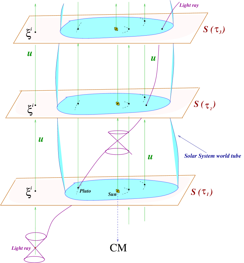
Figure 1: In our model each light ray behaves as if the bodies did not move with respect to the center of mass CM.

4 The light trajectories

A photon traveling from a distant star to the observer within the Solar System, would see the space-time as a time development of slices of constant $\tau$. As stated, we shall treat each light trajectory assuming that the bodies of the Solar System were fixed at the spatial position they had at the time of observation, say. Evidently, any subsequent light ray will be considered updating the positions of the bodies of the Solar System according to their actual motion. Let us then prepare the way to a suitable treatment of a light ray. Let

$$P(u)_{\alpha}{}^{\beta}=\delta_{\alpha}{}^{\beta}+u_{\alpha}u^{\beta}$$ (7)

be the operator which projects orthogonally to $\bm{u}$. Because of the unitary condition, the parameter $\sigma$ on the trajectories of $\bm{u}$ is not constant on the slices $S(\tau)$ but varies differentially with the position as $\sigma=\sigma(\xi^{i},\tau)$. Since the spatial coordinates $\xi^{i}$ are constant along the unique normal going through the point with those coordinates, the parameter $\sigma$ along it will be function of $\tau$ only; i.e. $\sigma=\sigma_{\xi^{i}}(\tau)$. Let us now consider a null geodesic $\mit\Upsilon$ with tangent vector field $k^{\alpha}\equiv d\xi^{\alpha}/d\lambda$ which satisfies the following equations:

$$k^{\alpha}k_{\alpha} = 0$$ (8)

$$\frac{dk^{\alpha}}{d\lambda}+{\Gamma}^{\alpha}_{\rho\sigma}k^{\rho}k^{\sigma} = 0;$$

the latter express respectively the null and the geodesic conditions; here $\lambda$ is a real parameter on $\mit\Upsilon$ and $\Gamma^{\alpha}_{\rho\sigma}$ are the connection coefficients of the given metric (Figure 2). Assume that the trajectory starts at a point $P_{\ast}$ on a slice $S(\tau_{*})$ (say) and with spatial coordinates $\xi_{*}^{i}$. The light trajectory will end at the observation place on a slice $S(\tau_{0})$ and at a point with spatial coordinates $\xi_{(0)}^{i}$. We remember that the origin of the coordinate system is meant to be the barycenter of the Solar System. The purpose of this work is to determine $\xi_{*}^{i}$, namely the coordinates of the star, from a prescribed set of observables.

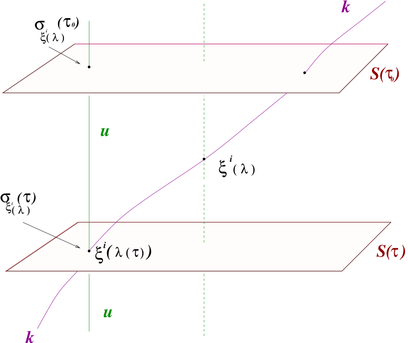
Figure 2: The point $\xi^{i}(\lambda(\tau))$ belongs to the null geodesic but also to the unique normal to the slice $S(\tau)$ crossing it with a value of the parameter $\sigma_{\xi^{i}(\lambda)}(\tau)$.

Since our approximation permits a global foliation of the space-time, we find it more convenient for the determination and physical interpretation of the gravitational effects on light propagation, to consider the spatial projection of the light ray $\mit\Upsilon$ on the slice $S(\tau_{0})$; this projection is a curve made of the points of $S(\tau_{0})$ which one gets to by moving along the unique normal through the point of intersection of the light ray with the slice $S(\tau)$, for any $\tau$. This curve, that we denote as $\bar{\mit\Upsilon}$, is smooth and has a tangent vector field ${\bf\ell}$ whose coordinate components are equal to those of the projection of the tangent ${\bf k}$ to the null ray into the rest frame of the local barycentric observer at each of its points, namely

$$\ell^{\alpha}=P(u)^{\alpha}{}_{\beta}k^{\beta}$$ (9)

(see Appendix A for a mathematical description of this mapping procedure). The vector ${\bf\ell}$ physically identifies the local line of sight of the local barycentric observer at each space-time point of the light ray trajectory. Indeed, the knowledge of ${\bf\ell}$ is essential to reconstruct the whole story of the light ray. The curve $\bar{\mit\Upsilon}$ will be naturally parametrized by $\lambda$.

From $u^{\alpha}u_{\alpha}=-1$, it follows that:

$$\ell^{\alpha}=k^{\alpha}+u^{\alpha}(u_{\beta}k^{\beta})\,.$$ (10)

Clearly it is $\ell^{0}=0$ showing that $\ell^{\alpha}$ lies everywhere on the slice $S(\tau_{0})$ as expected. Since each point of $\bar{\mit\Upsilon}$ is the image under the above projection operation of a point of $\mit\Upsilon$ at time $\tau$, it is more convenient to label the points of $\bar{\mit\Upsilon}$ with the value of the parameter $\sigma_{\xi^{i}(\lambda)}(\tau)$ which, as we have already said, uniquely identifies that point on the normal to the slice $S(\tau)$ which contains it. Hence, being

$$d\sigma=-(u_{\alpha}k^{\alpha})d\lambda\,,$$ (11)

we define the new tangent vector field:

$$\bar{\ell}^{\alpha}\equiv\frac{d\xi^{\alpha}}{d\sigma_{\xi^{i}(\lambda)}}=-\frac{\ell^{\alpha}}{\Big{(}u^{\beta}k_{\beta}\Big{)}}.$$ (12)

In the same way we denote

$$\bar{k}^{\alpha}\equiv-\frac{k^{\alpha}}{(u_{\beta}k^{\beta})}$$ (13)

so that

$$\bar{k}^{\alpha}=\bar{\ell}^{\alpha}+u^{\alpha}$$ (14)

which implies:

$$\bar{\ell}^{\alpha}\bar{\ell}_{\alpha}=1.$$ (15)

In what follows we shall denote $\sigma_{\xi^{i}(\lambda)}$ as $\sigma$. We can now write the differential equation which is satisfied by the vector field $\bar{\bm{\ell}}$. From (11) and (13), the second of equations (8) writes:

$$\frac{d\bar{\ell}^{\alpha}}{d\sigma} + \frac{du^{\alpha}}{d\sigma}-(\bar{\ell}^{\alpha}+u^{\alpha})(\bar{\ell}^{\beta}\dot{u}_{\beta}+\bar{\ell}^{\beta}\bar{\ell}^{\tau}\nabla_{\tau}u_{\beta})$$ (16)

$$+ \Gamma^{\alpha}_{\beta\gamma}(\bar{\ell}^{\beta}+u^{\beta})(\bar{\ell}^{\gamma}+u^{\gamma})=0\,.$$

In this equation the quantity $\bar{\ell}^{\beta}\bar{\ell}^{\tau}\nabla_{\tau}u_{\beta}$ can be written explicitly in terms of the expansion $\Theta_{\rho\sigma}$ of $C_{\bm{u}}$ (de Felice and Clarke, 1990), as:

$$\bar{\ell}^{\beta}\bar{\ell}^{\tau}\nabla_{\tau}u_{\beta}=\Theta_{\rho\sigma}\bar{\ell}^{\rho}\bar{\ell}^{\sigma}$$ (17)

where $\Theta_{\rho\sigma}=P(u)^{\alpha}{}\rho P(u)^{\beta}{}_{\sigma}\nabla_{(\alpha}u_{\beta)}$ Since the only non vanishing components of the expansion are $\Theta_{ij}=(1/2)\partial_{0}h_{ij}$, the expansion vanishes identically as consequence of the assumption to neglect time variations of the metric. From this condition and imposing $h_{0i}=0$ equation (16) becomes to the required order and after some algebra:

$$\frac{d\bar{\ell}^{\alpha}}{d\sigma} + \frac{1}{2}\left(\bar{\ell}^{i}\partial_{i}h_{00}\right)\delta^{\alpha}_{0}+\frac{1}{2}\left(\bar{\ell}^{i}\partial_{i}h_{00}\right)\left(\bar{\ell}^{\alpha}+\delta^{\alpha}_{0}\right)$$ (18)

$$+ \eta^{\alpha\sigma}\left(\partial_{i}h_{\sigma j}-\frac{1}{2}\partial_{\sigma}h_{ij}\right)\bar{\ell}^{i}\bar{\ell}^{j}+\eta^{\alpha\sigma}\left(\partial_{i}h_{0\sigma}\right)\bar{\ell}^{i}$$

$$- \frac{1}{2}\eta^{\alpha\sigma}\partial_{\sigma}h_{00}=0$$

If $\alpha=0$, equation (18) leads to $\frac{d\bar{\ell}^{0}}{d\sigma}=0$ assuring that condition $\bar{\ell}^{0}=0$ holds true all along the curve $\bar{\mit\Upsilon}$; if $\alpha=k$ equation (18) gives the set of differential equations that we need to integrate to identify the coordinate position of the star:

$$\frac{d\bar{\ell}^{k}}{d\sigma} + \bar{\ell}^{k}\left(\frac{1}{2}\bar{\ell}^{i}\partial_{i}h_{00}\right)+\delta^{ks}\left(\partial_{i}h_{sj}-\frac{1}{2}\partial_{s}h_{ij}\right)\bar{\ell}^{i}\bar{\ell}^{j}$$

$$- \frac{1}{2}\delta^{ks}\partial_{s}h_{00}=0,$$

$$\bar{\ell}^{k} = \frac{d\xi^{k}}{d\sigma}.$$ (19)

Here we remind that Latin indexes take values $1,2,3$.

5 Observables and boundary conditions

Our aim is to determine the coordinate positions of a star, from a prescribed set of observables. As first step we shall express the observables in a way which reflects a convenient set up for the observer. The latter carries a frame, namely a clock which measures its proper-time and a rest-space, which are different from the barycentric proper-time and rest-space, respectively given by the parameter $\sigma(\tau)$ along the congruence $C_{\bm{u}}$ and the space-like slices $S(\tau)$. To determine the boundary conditions needed to integrate equation (19), we need both frames; the observer frame allows us to define the measurements and the barycentric one to express all the coordinate tensorial components. Each measurement is made at a coordinate time $\tau_{0}$ when the observer was at a spatial position with respect to the barycenter given by the coordinates $\xi^{i}_{(0)}$. Hence we consider as observables the angles between the direction of the incoming photon and the three spatial directions of a frame adapted to the observer. These three angles provide the required boundary values for $\bar{\ell}^{i}$. Let $\bm{u^{\prime}}$ be the vector field tangent to the observer’s world-line and let $\{\bm{\lambda_{\hat{a}}}\}$ (where $\hat{a}=1,2,3$) be a space-like triad carried by the observer. The angles $\psi_{(\lambda_{\hat{a}},\bar{\ell})}$ that the incoming light ray forms with each of the triad direction, is given by (de Felice and Clarke, 1990):

$$\cos\psi_{(\lambda_{\hat{a}},\bar{\ell})}\equiv\textbf{e}\bm{{}^{\prime}_{\hat{a}}}=\frac{\gamma^{\prime}_{\alpha\beta}\bar{k}^{\alpha}\lambda^{\beta}_{\hat{a}}}{(\gamma^{\prime}_{\alpha\beta}\bar{k}^{\alpha}\bar{k}^{\beta})^{1/2}(\gamma^{\prime}_{\alpha\beta}\lambda^{\alpha}_{\hat{a}}\lambda^{\beta}_{\hat{a}})^{1/2}}$$ (20)

where no sum is meant over $\hat{a}$ and ${\gamma^{\prime}_{\alpha}}^{\beta}=\delta_{\alpha}^{\beta}+u^{{}^{\prime}\beta}u^{\prime}_{\alpha}$ is the operator which projects into the observer’s rest-frame (Figure 3).

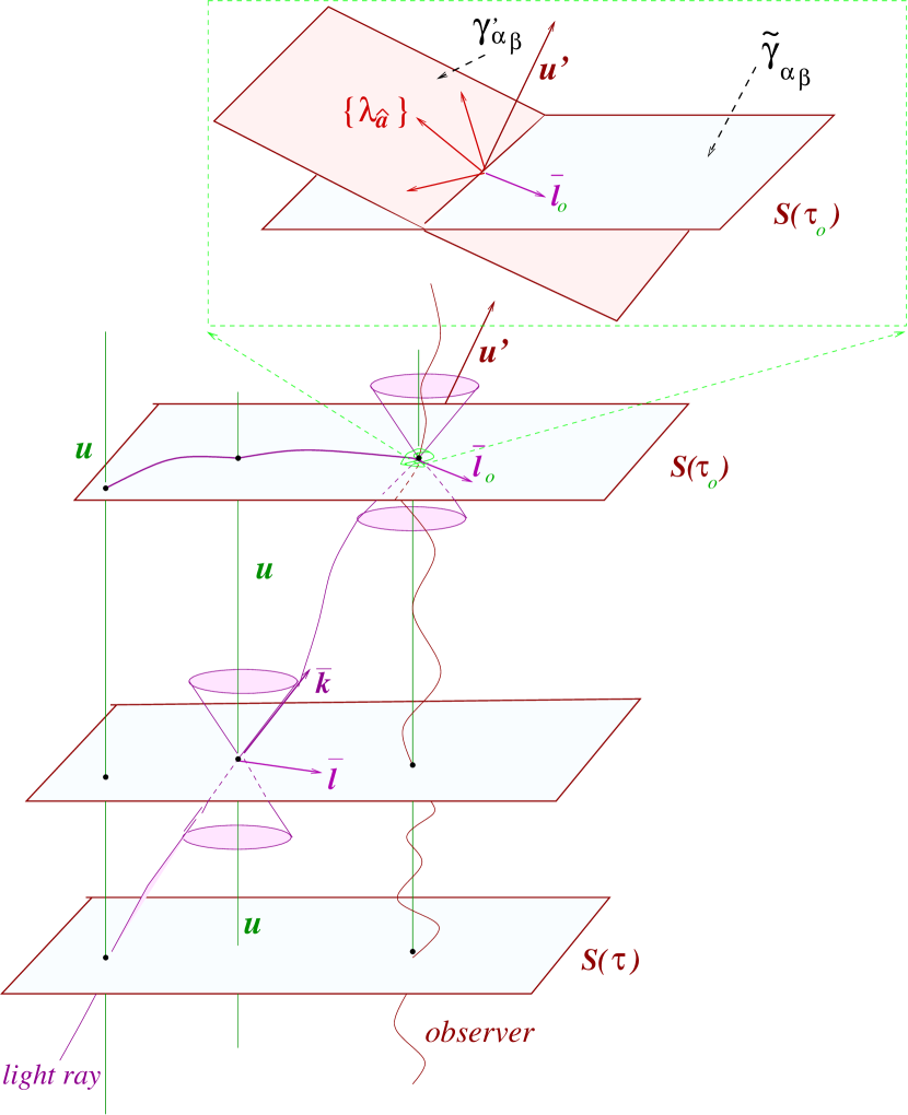
Figure 3: Fixing the boundary condition at the time of the observation $\tau_{0}$, where $u^{\prime}$ is the tangent vector to the world line of the observer.

From (14), the above equation can be written more conveniently as

$$\textbf{e}\bm{{}^{\prime}_{\hat{a}}}=\frac{\bar{\ell}^{i}_{0}\lambda_{i\hat{a}}+u^{\beta}\lambda_{\beta\hat{a}}}{{u^{\prime}}_{j}\bar{\ell}_{0}^{j}+u^{{}^{\prime}\rho}u_{\rho}}$$ (21)

where $\bar{\ell}_{0}\equiv\bar{\ell}(\tau_{0})$ and recalling that $\gamma^{\prime}_{\alpha\beta}\lambda^{\alpha}_{\hat{a}}\lambda^{\beta}_{\hat{a}}=1$; this is a matrix equation where the unknowns are the photon’s spatial directions $\bar{l}^{k}_{0}$ at the time of observation; they can be singled out as

$$\bar{\ell}^{i}_{0}[u^{\prime}_{i}\textbf{e}\bm{{}^{\prime}_{\hat{a}}}-\lambda_{i\hat{a}}]=u^{\alpha}\lambda_{\hat{a}\alpha}-\textbf{e}\bm{{}^{\prime}_{\hat{a}}}(u^{{}^{\prime}\alpha}u_{\alpha}).$$ (22)

The direction of the light ray, as it is seen from the point of observation, depends on the motion of the latter relative to the center of mass. This dependence gives rise to the stellar aberration. Did the observer not move with respect to the spatial coordinate grid, namely if $u^{{}^{\prime}\alpha}=u^{\alpha}$, then (22) would become $\bar{\ell}^{i}_{0}\lambda_{i\hat{a}}=\textbf{e}\bm{{}_{\hat{a}}}$ as expected. Equations (19) and the three conditions (22) together with equations (12) and the coordinate positions $\xi^{i}_{(o)}=\xi^{i}(\tau_{o})$ of the observer at the time of observation, form a closed system of equations whose solutions are the coordinate positions of the star provided one is able to identify the value of the parameter $\sigma$ at the emission. The solution of (19), in fact, is of the type $\xi^{i}(\sigma,\,\bar{\ell}_{0}^{i},\,\xi_{(o)}^{i})$ hence $\sigma_{*}\equiv\sigma(\tau_{*})$ which marks the photon emission, is an implicit unknown. The way how to determine $\sigma_{*}$ will be discussed in the following section.

In order to find the boundary conditions $\bar{\ell}^{i}_{0}$ for equations (19), we have first to construct a tetrad frame adapted to the observer. The tetrad frame {$\bm{\lambda_{\hat{\alpha}}}$} forms a system of local Cartesian axes, which equips the observer with an instantaneous inertial frame; in fact it is:

$$\left(\bm{\lambda_{\hat{\alpha}}}\mid\bm{\lambda_{\hat{\beta}}}\right)=\eta_{\hat{\alpha}\hat{\beta}}.$$ (23)

Let us relabel for convenience the coordinates $\xi^{\alpha}$ as $(\tau,\,x,\,y,\,z)$; each tetrad vector $\bm{\lambda_{\hat{\alpha}}}$ can then be expressed in terms of coordinate components with respect to the coordinate basis, as:

$$\bm{u^{\prime}}\equiv\bm{\lambda_{\hat{0}}} = \rm{e}^{\psi^{\prime}}\left(T_{s}\bm{\partial_{0}}+X_{s}\bm{\partial_{x}}+Y_{s}\bm{\partial_{y}}+Z_{s}\bm{\partial_{z}}\right)$$ (24)

$$\bm{\lambda_{\hat{a}}} = T_{a}\bm{\partial_{0}}+X_{a}\bm{\partial_{x}}+Y_{a}\bm{\partial_{y}}+Z_{a}\bm{\partial_{z}}$$ (25)

where $\rm{e}^{\psi^{\prime}}$ is the normalization function which makes $\bm{u^{\prime}}$ unitary and $a=1,\,2,\,3$. Conditions (23) must be simultaneously satisfied hence after some algebra we obtain:

$$\rm{e}^{\psi^{\prime}}=\left[-\left(T_{s}^{2}g_{00}+X_{s}^{2}g_{xx}+Y_{s}^{2}g_{yy}+Z_{s}^{2}g_{zz}\right)\right]^{-1/2}.$$ (26)

and

$$T_{s}T_{a}g_{00}+X_{s}X_{a}g_{xx}+Y_{s}Y_{a}g_{yy}+Z_{s}Z_{a}g_{zz}=0$$ (27)

$$T_{a}T_{b}g_{00}+X_{a}X_{b}g_{xx}+Y_{a}Y_{b}g_{yy}+Z_{a}Z_{b}g_{zz}=0$$ (28)

$$T_{a}^{2}g_{00}+X_{a}^{2}g_{xx}+Y_{a}^{2}g_{yy}+Z_{a}^{2}g_{zz}=1$$ (29)

where $a\neq b$. A general solution of (27–29) is given by:

$$\bm{\lambda_{\hat{0}}} = \rm{e}^{\psi^{\prime}}\left(\bm{\partial}_{0}+X_{s}\bm{\partial_{x}}+Y_{s}\bm{\partial_{y}}+Z_{s}\bm{\partial_{z}}\right)$$ (30)

$$\bm{\lambda_{\hat{1}}} = X_{1}\bm{\partial_{x}}+Y_{1}\bm{\partial_{y}}$$ (31)

$$\bm{\lambda_{\hat{2}}} = T_{2}\bm{\partial_{0}}+X_{2}\bm{\partial_{x}}+Y_{2}\bm{\partial_{y}}+Z_{2}\bm{\partial_{z}}$$ (32)

$$\bm{\lambda_{\hat{3}}} = T_{3}\bm{\partial_{0}}+Z_{3}\bm{\partial_{z}}$$ (33)

where the components are explicitly given in Appendix B. This solution describes the instantaneous inertial frame of an observer endowed with a general motion in a gravitational field described by metric (2).

It is crucial that our model is consistent, under the same conditions, with the one discussed in de Felice et al. (1998) and de Felice et al. (2001) where the Sun was the only source of gravity. In order to make comparison easier let us assume that the observer moves on a circular orbit around the barycenter of the Sun-Earth system and has, at the time of observation, spatial coordinates $x_{0},y_{0},$ and $z_{0}=0$. The 4-velocity of the observer now reads:

$$\bm{u}^{{}^{\prime}\alpha}=\rm{e}^{\psi^{\prime}}\left(\bm{\partial_{0}}-\omega(y_{0}-y_{\odot})\bm{\partial_{x}}+\omega(x_{0}-x_{\odot})\bm{\partial_{y}}\right)$$ (34)

where $\omega$ is the coordinate Keplerian angular velocity of revolution and ($x_{\odot},\,y_{\odot}$) are the coordinates of the barycenter of the Sun-Earth with respect to the barycenter of the Solar System. In this case, the tetrad frame becomes:

$$\bm{\lambda_{\hat{0}}}\!\! = \!\!\rm{e}^{\psi^{\prime}}\left(\bm{\partial_{0}}-\omega(y_{0}-y_{\odot})\bm{\partial_{x}}+\omega(x_{0}-x_{\odot})\bm{\partial_{y}}\right)$$ (35)

$$\bm{\lambda_{\hat{1}}}\!\! = \!\!X_{1}\bm{\partial_{x}}+Y_{1}\bm{\partial_{y}}$$ (36)

$$\bm{\lambda_{\hat{2}}}\!\! = \!\!T_{2}\bm{\partial_{0}}+X_{2}\bm{\partial_{x}}+Y_{2}\bm{\partial_{y}}$$ (37)

$$\bm{\lambda_{\hat{3}}}\!\! = \!\!Z_{3}\bm{\partial_{z}}$$ (38)

where:

$$\rm{e}^{\psi^{\prime}}\!\!=\!\!\left[-\!\left(g_{00}\!+\!\omega^{2}(y_{0}\!-\!y_{\odot})^{2}g_{xx}\!+\!\omega^{2}(x_{0}\!-\!x_{\odot})^{2}g_{yy}\right)\right]^{-1/2},$$ (39)

$$X_{1} = -\frac{\sqrt{g_{yy}}\,(x_{0}-x_{\odot})}{\sqrt{g_{xx}}\sqrt{\Sigma}},$$ (40)

$$Y_{1} = -\frac{\sqrt{g_{xx}}\,(y_{0}-y_{\odot})}{\sqrt{g_{yy}}\sqrt{\Sigma}},$$ (41)

$$T_{2} = \frac{\omega\sqrt{\Sigma}}{\sqrt{-g_{00}}\sqrt{-\Pi}},$$ (42)

$$X_{2} = -\frac{(y_{0}-y_{\odot})\sqrt{-g_{00}}}{\sqrt{\Sigma}\sqrt{-\Pi}},$$ (43)

$$Y_{2} = \frac{(x_{0}-x_{\odot})\sqrt{-g_{00}}}{\sqrt{\Sigma}\sqrt{-\Pi}},$$ (44)

$$Z_{3} = -\frac{1}{\sqrt{g_{zz}}},$$ (45)

and where we have named:

$$\Sigma = g_{xx}(y_{0}-y_{\odot})^{2}+g_{yy}(x_{0}-x_{\odot})^{2}$$

$$\Pi = g_{00}+\left[g_{xx}(y_{0}-y_{\odot})^{2}+g_{yy}(x_{0}-x_{\odot})^{2}\right]\omega^{2}.$$

We can now solve the system (22) explicitly, relating the observed quantities $\textbf{e}\bm{{}^{\prime}_{\hat{a}}}$ to the unknowns $\bar{\ell}^{\alpha}_{0}$ by means of the observer’s comoving frame { $\bm{\lambda_{\hat{\alpha}}}$ }, i.e.:

$$\bar{\ell}_{0}^{x} = \frac{1}{\sqrt{g_{xx}}\sqrt{\Sigma}}\left[\frac{\textbf{e}\bm{{}^{\prime}_{\hat{1}}}(x_{0}-x_{\odot})\sqrt{g_{yy}}\sqrt{-\Pi}+(y_{0}-y_{\odot})\sqrt{g_{xx}}(\omega\sqrt{\Sigma}+{\textbf{e}\bm{{}^{\prime}_{\hat{2}}}}\sqrt{-g_{00}})}{(\textbf{e}\bm{{}^{\prime}_{\hat{2}}}\omega\sqrt{\Sigma}-\sqrt{-g_{00}})}\right]$$ (46)

$$\bar{\ell}_{0}^{y} = \frac{1}{\sqrt{g_{yy}}\sqrt{\Sigma}}\left[\frac{\textbf{e}\bm{{}^{\prime}_{\hat{1}}}(y_{0}-y_{\odot})\sqrt{g_{xx}}\sqrt{-\Pi}-(x_{0}-x_{\odot})\sqrt{g_{yy}}(\omega\sqrt{\Sigma}+\textbf{e}\bm{{}^{\prime}_{\hat{2}}}\sqrt{-g_{00}})}{(\textbf{e}\bm{{}^{\prime}_{\hat{2}}}\omega\sqrt{\Sigma}-\sqrt{-g_{00}})}\right]$$ (47)

$$\bar{\ell}^{z}_{0} = -\frac{\textbf{e}\bm{{}^{\prime}_{\hat{3}}}\,\sqrt{-\Pi}}{\sqrt{g_{zz}}\left(\textbf{e}\bm{{}^{\prime}_{\hat{2}}}\omega\sqrt{\Sigma}-\sqrt{-g_{00}}\right).}$$ (48)

6 Identifying the emission time

Let us assume that the star has no proper motion with respect to the given spatial coordinate grid whose origin is at the barycenter of the Solar System. In this case the spatial coordinates $\xi^{i}_{*}\equiv\xi^{i}(\tau_{*})$ of the star remain fixed with time $\tau$ and the star’s world-line is one of the curves of the congruence $C_{\bm{u}}$. If a photon is emitted at $\tau_{*}$, say, then its trajectory all the way to the observer at ($\xi^{i}_{(0)},\,\tau_{0}$) is mapped into a spatial path on the slice $S(\tau_{0})$ having the boundary conditions fixed as explained in Section 4. Integration along this path leads to a solution $\xi^{i}=\xi^{i}(\sigma(\tau))$. Let the same star be observed at a subsequent coordinate time $\tau^{\prime}_{0}=\tau_{0}+\Delta\tau$; the received photon is emitted at a coordinate time $\tau^{\prime}_{*}=\tau_{*}+\Delta\tau$ and its trajectory is now mapped into a slice $S(\tau^{\prime}_{0})$. Evidently, this second observation implies a different set of boundary conditions for the integration along the second path hence the solution will be a new function $\xi^{i^{\prime}}=\xi^{i^{\prime}}(\sigma(\tau))$. Since the spatial coordinates of the star are preserved under the mapping, they will be identified by the value of the parameter $\sigma(\tau_{*})$ such that $\xi^{{}^{\prime}i}(\sigma(\tau_{*}+\Delta\tau))=\xi^{i}(\sigma(\tau_{*}))$ (see Figure 4).

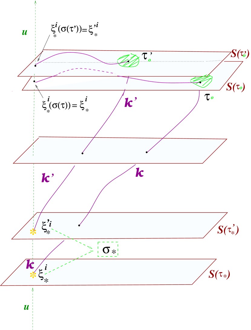
Figure 4: Identifying the coordinate position $\xi^{i}_{*}$ of the star without proper motion and the emission time $\sigma(\tau_{*})$.

A first check of the procedure is shown in Figure 5; here we assume that on the light path acts only the gravitational field of the Sun. We considered two stars at coordinate distances respectively of 1 and 2 parsecs. Fixing the boundary conditions corresponding to observations of the stars in two symmetrically opposite directions with respect to the Sun and assuming $\Delta\tau$ equal to six months, we find, in logarithmic units, the points of intersections of the two integrated spatial paths. The actual distances are slightly less that 1 and 2 parsecs respectively as expected since we calculate proper rather coordinate distances.

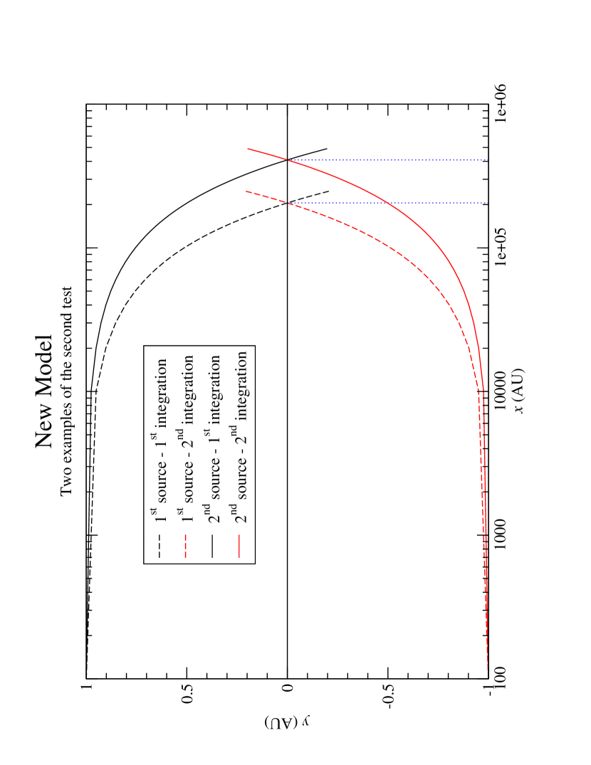
Figure 5: Two examples of a test that deduces the distance of a star from two observations of the same objects taken at opposite positions on the orbit of the observer. The first star is approximately at 1 parsec, the second at 2 parsecs. Each couple of observations gives two trajectories that cross at the expected distance of the objects.

7 Testing the model

The perturbative model presented in the last chapter is expected to include all terms to the order of $(v/c)^{2}$. This means that, for a typical velocity in the solar system of $\sim 10~{}\rm{km}\cdot\rm{s}^{-1}$, one can expect deviations from the predictions of exact models of $\simeq 2\cdot 10^{-4}~{}\rm{arcsec}$. Equations (19) cannot be integrated analytically, so numerical techniques are needed to reconstruct the light path. We then needed a test campaign to check the correctness and accuracy of the model.

We used the implementation of the RADAU integrator given in (Everhart, 1985) to integrate the system of differential equations for the null geodesic, because it has been thoroughly tested, and can be easily implemented to reach very high orders of accuracy. Since the geodesic equations include both $\bar{\ell}^{i}\equiv\dot{\xi}^{i}$ and $\xi^{i}$, the system of differential equations is of class II according to the definition used in (Everhart, 1985), that is

$$\textbf{y}^{\prime\prime}=F(\textbf{y}^{\prime},\textbf{y},t).$$

The tests we devised verify that:

1. the perturbative model is self-consistent;

2. the amount of light deflection caused by each individual body of the Solar System, as evaluated in our perturbative model, coincides with that expected for an analytical Schwarzschild solution at the same order of accuracy and under the same observational conditions;

3. the model is able to reconstruct stellar distances.

It is clear from these items that our tests do not consider comparisons with other models besides the Schwarzschild solution, like those in Kopeikin and Mashhoon (2002) and Klioner (2003); however, we believe that it is still too early for such comparisons. First of all, our model is at the $(v/c)^{2}$ order, so it’s not strictly needed to confront it with higher order models yet. Moreover, although with the same assumptions some results can be recovered, the background mathematical framework is quite different and this is another reason for not attempting a detailed comparison. Our model is evolving to the $(v/c)^{3}$ order, and this future version will be presented in a forthcoming paper and, indeed, compared to the two works cited above.

Before illustrating each specific test, let us make some general remarks on the numerical solution of the system of differential equations (19). This system requires a set of six boundary conditions and, as said in section 5, the natural choice is the three spatial coordinates of the observer at the observation time, and the three components of the vector tangent to the spatial line of sight.

We are dealing with a numerical problem, therefore we need to define methods to stop the integration procedure.

One possibility is to fix a finite range of integration, the starting point being the position of the observer and the ending point that of the star. This approach will be adopted for the test on stellar distances.

The other choice is to stop the integration when the tangent vector to the light trajectory becomes constant at the precision level of the computer. This method was used in the light deflection test. In particular, when we consider only the gravitational field generated by the Sun, the total amount of deflection produced beyond 100 AU is under $0.1~{}\mu$arcsec level, therefore this distance turns out to be a pretty good choice for stopping the integration.

As a final consideration, we mention that the geodesic equations can be adapted to various physical situations; in fact, as explained in section 2, the metric has not been explicited the only requirement being that it takes the form:

$$g_{\alpha\beta}=\eta_{\alpha\beta}+h_{\alpha\beta}+O(h^{2}).$$

In our approximation it is

$$(\eta_{\alpha\beta}+h_{\alpha\beta})\bar{\ell}^{\alpha}\bar{\ell}^{\beta}=1+O((v/c)^{3}),$$

so the first step was to verify whether the spatial vectors $\bar{\ell}$ obtained at each step of integration satisfied this unitarity condition up to the correct order of accuracy of $\sim 10^{-12}$. The results show that this always happens along the integration path.

7.1 Self-consistency test

The basic test is whether our model satisfies spherical symmetry in the case that the Sun is the only source of gravity.

Therefore, we took the $(v/c)^{2}$ approximation of the Schwarzschild metric; the fundamental property of this space-time solution is its spherical symmetry. This means that the amount of light deflection measured by an observer in a given position must depend only on the angular distance of the celestial object from the gravitational source.

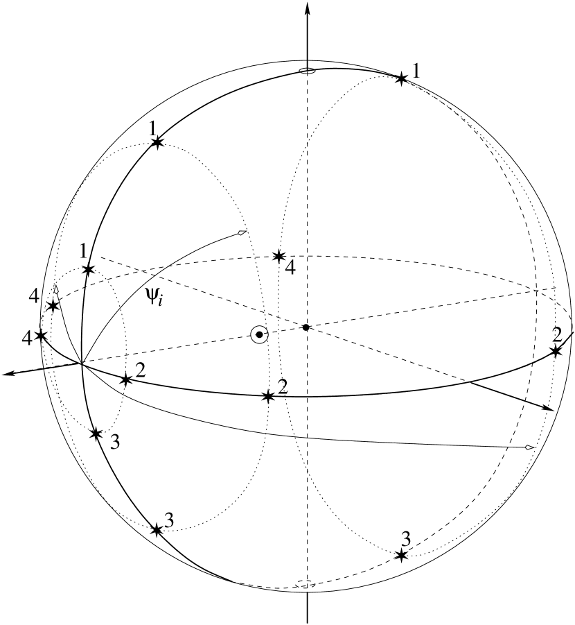
Figure 6: Geometry taken for the self-consistency test. For each $\psi$ there are four stars at symmetric positions with respect to the Sun-observer direction. The angle $\psi$ goes from $\sim 16^{\prime\prime}$ (i.e. limb-grazing rays) to nearly $180^{\circ}$. The observer is located at the origin of the reference frame.

We considered an observer at $r_{0}=1$ AU and a set of stars placed at different angular distances $\psi$ from the Sun. For each $\psi$, we have taken four stars symmetrically positioned with respect to the Sun as in Figure 6.

The results are reported in Table 1 where $\delta\psi_{i}$ are the deflections calculated in the four cases. They were calculated to the $0.1$ $\mu$arcsec level and, as expected, are the same for a given angular distance: this is a verification of the physical consistency of the model.

The way we calculated the light deflections is discussed below.

Table 1: Results for the self-consistency tests. $\psi$ is the angular distance from the Sun, $\delta\psi_{1}\ldots\delta\psi_{4}$ the deflection obtained in four symmetric cases at the same $\psi$ (only one value is reported here for each $\psi$ since they are exactly the same for each $\delta\psi_{i}$.

$\psi$	$\delta\psi_{1}\,\ldots\,\delta\psi_{4}$
$\phantom{0}\phantom{0}0^{\circ}16^{\prime}\phantom{0}5^{\prime\prime}\!\!.1428100$	$1^{\prime\prime}\!\!.7406216$
$\phantom{0}\phantom{0}1^{\circ}\phantom{0}0^{\prime}\phantom{0}0^{\prime\prime}\!\!.0\phantom{000000}$	$0^{\prime\prime}\!\!.4666385$
$\phantom{0}\phantom{0}2^{\circ}\phantom{0}0^{\prime}\phantom{0}0^{\prime\prime}\!\!.0\phantom{000000}$	$0^{\prime\prime}\!\!.2333012$
$\phantom{0}\phantom{0}5^{\circ}\phantom{0}0^{\prime}\phantom{0}0^{\prime\prime}\!\!.0\phantom{000000}$	$0^{\prime\prime}\!\!.0932707$
$\phantom{0}10^{\circ}\phantom{0}0^{\prime}\phantom{0}0^{\prime\prime}\!\!.0\phantom{000000}$	$0^{\prime\prime}\!\!.0465464$
$\phantom{0}45^{\circ}\phantom{0}0^{\prime}\phantom{0}0^{\prime\prime}\!\!.0\phantom{000000}$	$0^{\prime\prime}\!\!.0098314$
$\phantom{0}60^{\circ}\phantom{0}0^{\prime}\phantom{0}0^{\prime\prime}\!\!.0\phantom{000000}$	$0^{\prime\prime}\!\!.0070534$
$\phantom{0}75^{\circ}\phantom{0}0^{\prime}\phantom{0}0^{\prime\prime}\!\!.0\phantom{000000}$	$0^{\prime\prime}\!\!.0053071$
$\phantom{0}85^{\circ}\phantom{0}0^{\prime}\phantom{0}0^{\prime\prime}\!\!.0\phantom{000000}$	$0^{\prime\prime}\!\!.0044441$
$\phantom{0}95^{\circ}\phantom{0}0^{\prime}\phantom{0}0^{\prime\prime}\!\!.0\phantom{000000}$	$0^{\prime\prime}\!\!.0037316$
$105^{\circ}\phantom{0}0^{\prime}\phantom{0}0^{\prime\prime}\!\!.0\phantom{000000}$	$0^{\prime\prime}\!\!.0031248$
$120^{\circ}\phantom{0}0^{\prime}\phantom{0}0^{\prime\prime}\!\!.0\phantom{000000}$	$0^{\prime\prime}\!\!.0023511$
$135^{\circ}\phantom{0}0^{\prime}\phantom{0}0^{\prime\prime}\!\!.0\phantom{000000}$	$0^{\prime\prime}\!\!.0016868$
$170^{\circ}\phantom{0}0^{\prime}\phantom{0}0^{\prime\prime}\!\!.0\phantom{000000}$	$0^{\prime\prime}\!\!.0003563$
$175^{\circ}\phantom{0}0^{\prime}\phantom{0}0^{\prime\prime}\!\!.0\phantom{000000}$	$0^{\prime\prime}\!\!.0001778$
$179^{\circ}43^{\prime}54^{\prime\prime}\!\!.8571900$	$0^{\prime\prime}\!\!.0000095$

7.1.1 Numerical calculation of the light deflection

The integrator takes as boundary conditions the Cartesian coordinates of the observer at the time of observation and the component of the unit vector representing the direction of the line of sight (that is the tangent unit vector to the light path at the moment of observation). The quantities $\mathbf{\xi}$ and $\dot{\mathbf{\xi}}$ are recalculated at each step of integration, so the total light deflection angle is the angle between the viewing direction $\bar{\ell}^{i}_{0}$ at the observation time and the direction $\bar{\ell}^{i}_{f}$ of the unit vector tangent to the light path at the end of integration (Figure 7).

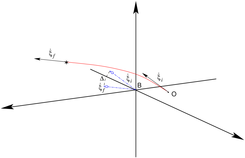
Figure 7: The deflection angle $\Delta$ is the angle between the initial viewing direction $\mathbf{\dot{\xi}}_{i}$ and the final tangent unit vector at the end of the integration to the light path $\mathbf{\dot{\xi}}_{f}$ but parallely propagated along the light trajectory to the observation point.

The most straightforward formula for the computation of an angle between two direction would be just

$$\Delta=\arccos(\mathbf{v}|\mathbf{w}),$$ (49)

where $\mathbf{v}$ and $\mathbf{w}$ are any two given unit tangent vectors. Unfortunately, from a numerical point of view, this formula is of little utility, because of the smallness of the deflection angle. In fact the numerical accuracy that we need for $\Delta$ is $\delta\Delta\sim 1~{}\mu$arcsec, but for angles as small as those expected for the relativistic deflections, namely $\Delta\lesssim 2~{}$arcsec, the accuracy of the built-in $\arccos$ function drops at the $10^{-4}~{}$arcsec level. Let us show this with a simple test. Consider two points $\mathsf{R}_{1}$ and $\mathsf{R}_{2}$ on the unit celestial sphere with polar coordinates $(\alpha_{1},\delta_{1})$ and $(\alpha_{2},\delta_{2})$, and let $\alpha_{1}=\delta_{1}=\delta_{2}=0$ and $\alpha_{2}$ variable. Then the angle $\Delta$ between the two directions v and w pointing to them is simply given by $\alpha_{2}$. However, application of formula (49) leads to the results with poor accuracy shown in Table 2.

Table 2: Test for the accuracy of the arccos function for small angles. The angular coordinates of two points are given as follows: the first one has $\alpha_{1}=\delta_{1}=0$, the second one has $\delta_{2}=0$ while $\alpha_{2}$ decreases. The angle $\Delta$ between the two directions $\mathbf{v}$ and $\mathbf{w}$ pointing to $\mathsf{R}_{1}$ and $\mathsf{R}_{2}$ is exactly given by $\alpha_{2}$, but is also calculated taking the arccos of the scalar product of the two unit vectors. The results show that when $\Delta\sim 10^{-1}~{}$arcsec the accuracy of the built-in arccos is less than $1~{}\mu$arcsec.

$\Delta=\alpha_{2}~{}(^{\prime\prime})$	$\arccos~{}(^{\prime\prime})$	$\Delta-\arccos~{}(\mu\rm{arcsec})$
3240.003043	3240.003043	000.000
0324.000304	0324.000304	0-0.001
0032.400030	0032.400031	0-0.069
0003.240003	0003.240004	0-0.485
0000.324000	0000.323998	002.721
0000.032400	0000.032382	017.771
0000.003240	0000.003074	166.415
0000.000324	0000.000000	324.000

A solution to this problem is to consider an approximate formula for $\Delta$ which is better suitable for our case. From spherical trigonometry the exact formulas for the angular distance $\Delta$ and the position angle $p$ of two points on the unit celestial sphere (Figure 8) $\mathsf{R}_{1}=(\alpha_{1},\delta_{1})$ and $\mathsf{R}_{2}=(\alpha_{2},\delta_{2})$ are

$$\sin\!\Delta\sin\!p\!\! = \!\!\cos\!\delta_{2}\sin(\alpha_{2}-\alpha_{1})$$ (50)

$$\sin\!\Delta\cos\!p\!\! = \!\!\sin\!\delta_{2}\cos\!\delta_{1}\!-\!\cos\!\delta_{2}\sin\!\delta_{1}\cos(\alpha_{2}\!-\!\alpha_{1}).$$ (51)

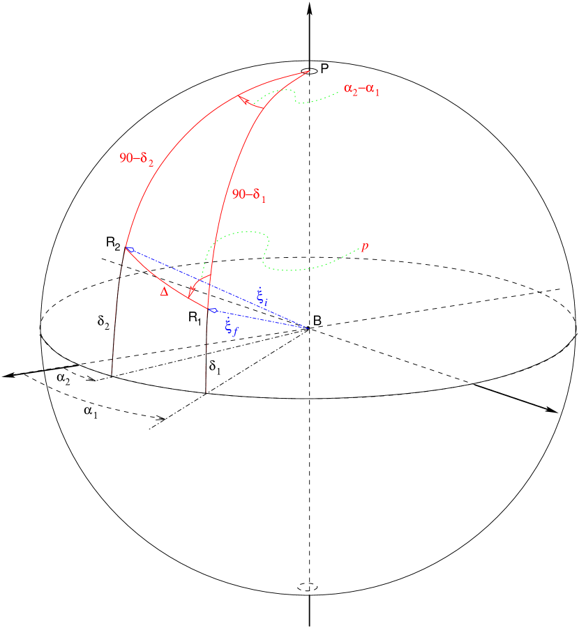
Figure 8: Angular distance $\Delta$ between two points $\mathsf{R}_{1}=(\alpha_{1},\delta_{1})$ and $\mathsf{R}_{2}=(\alpha_{2},\delta_{2})$. Here P is the pole of the celestial sphere and $p$ is the position angle of $\mathsf{R}_{2}$ with respect to $\mathsf{R}_{1}$.

The Taylor series of the sine and cosine functions about $x=0$ are

$$\sin x = x-\frac{x^{3}}{6}+\frac{x^{5}}{120}+\mathcal{O}(x^{7})$$ (52)

$$\cos x = 1-\frac{x^{2}}{2}+\frac{x^{4}}{24}+\mathcal{O}(x^{6}).$$ (53)

For $x\simeq 2~{}\rm{arcsec}\simeq 10^{-5}~{}\rm{rad}$, $x^{2}\simeq 10^{-10}~{}\rm{rad}\sim 10~{}\mu\rm{arcsec}$ and $x^{3}\simeq 10^{-15}~{}\rm{rad}\sim 2\cdot 10^{-4}~{}\mu\rm{arcsec}$ we can write $\forall~{}x\lesssim 2~{}\rm{arcsec}$

$$\sin x = x+\mathcal{O}(10^{-3}\mu\rm{arcsec})$$ (54)

$$\cos x = 1-\frac{x^{2}}{2}+\mathcal{O}(10^{-8}\mu\rm{arcsec})).$$ (55)

Let’s now write $\alpha_{2}-\alpha_{1}=\zeta\lesssim 10^{-5}~{}\rm{rad}$ and $\delta_{2}-\delta_{1}=\epsilon\lesssim 10^{-5}~{}\rm{rad}$. The right-hand side of the (51) can be re-written, to the correct accuracy, as

$$\sin\delta_{2}\cos\delta_{1}-\cos\delta_{2}\sin\delta_{1}\cos(\alpha_{2}-\alpha_{1})$$ (56)

$$\simeq \sin\delta_{2}\cos\delta_{1}-\cos\delta_{2}\sin\delta_{1}\left(1-\frac{\zeta^{2}}{2}\right)$$

$$= \sin(\delta_{2}-\delta_{1})+\frac{1}{2}\zeta^{2}\cos\delta_{2}\sin\delta_{1}$$

$$\simeq (\delta_{2}-\delta_{1})+\frac{1}{2}\cos\delta_{2}\sin\delta_{1}$$

The system of equations (50) and (51) can then be approximated as

$$\Delta\,\sin p = (\alpha_{2}-\alpha_{1})\cos\delta_{2}$$ (57)

$$\Delta\,\cos p = (\delta_{2}-\delta_{1})+\frac{1}{2}\cos\delta_{2}\sin\delta_{1}$$ (58)

so

$$\Delta^{2} = (\alpha_{2}-\alpha_{1})^{2}\cos^{2}\delta_{2}+(\delta_{2}-\delta_{1})^{2}+$$ (59)

$$\frac{1}{2}\zeta^{2}(\delta_{2}-\delta_{1})\cos\delta_{2}\sin\delta_{1}+\frac{1}{4}\zeta^{4}\cos^{2}\delta_{2}\sin^{2}\delta_{1}$$

$$= (\alpha_{2}-\alpha_{1})^{2}\cos^{2}\delta_{2}+(\delta_{2}-\delta_{1})^{2}+\mathcal{O}(\zeta^{3}).$$

This is the formula that we shall use to compute the angle between any two vectors

.

Table 3: Results for the light deflection test. The deflection $\Delta_{m}$ is computed with a formula for the Schwarzschild metric for increasing values of the angular displacement $\psi$ of the light source from the Sun. This value is compared with that deduced from our model, ($\Delta$). The difference $\Delta-\Delta_{m}$ goes rapidly under the $0.1~{}\mu$arcsec level for $\psi>5^{\circ}$, and the magnitude of its maximum value is well within that expected for the $(v/c)^{2}$ approximation.

$\psi$			$\Delta$	$\Delta_{m}$	$\Delta-\Delta_{m}(\mu$arcsec$)$
$0^{\circ}$	$16^{\prime}$	$\phantom{0}5^{\prime\prime}\!\!.1428100$	$1^{\prime\prime}\!\!.7406216$	$1^{\prime\prime}\!\!.7406073$	$14.3$
$1^{\circ}$	$0^{\prime}$	$\phantom{0}0^{\prime\prime}\!\!.0$	$0^{\prime\prime}\!\!.4666385$	$0^{\prime\prime}\!\!.4666375$	$\phantom{0}1.0$
$2^{\circ}$	$0^{\prime}$	$\phantom{0}0^{\prime\prime}\!\!.0$	$0^{\prime\prime}\!\!.2333012$	$0^{\prime\prime}\!\!.2333010$	$\phantom{0}0.2$
$5^{\circ}$	$0^{\prime}$	$\phantom{0}0^{\prime\prime}\!\!.0$	$0^{\prime\prime}\!\!.0932707$	$0^{\prime\prime}\!\!.0932706$	$\phantom{0}0.1$
$10^{\circ}$	$0^{\prime}$	$\phantom{0}0^{\prime\prime}\!\!.0$	$0^{\prime\prime}\!\!.0465464$	$0^{\prime\prime}\!\!.0465464$	$\phantom{0}0.0$
$45^{\circ}$	$0^{\prime}$	$\phantom{0}0^{\prime\prime}\!\!.0$	$0^{\prime\prime}\!\!.0098314$	$0^{\prime\prime}\!\!.0098314$	$\phantom{0}0.0$
$60^{\circ}$	$0^{\prime}$	$\phantom{0}0^{\prime\prime}\!\!.0$	$0^{\prime\prime}\!\!.0070534$	$0^{\prime\prime}\!\!.0070534$	$\phantom{0}0.0$
$75^{\circ}$	$0^{\prime}$	$\phantom{0}0^{\prime\prime}\!\!.0$	$0^{\prime\prime}\!\!.0053071$	$0^{\prime\prime}\!\!.0053071$	$\phantom{0}0.0$
$85^{\circ}$	$0^{\prime}$	$\phantom{0}0^{\prime\prime}\!\!.0$	$0^{\prime\prime}\!\!.0044441$	$0^{\prime\prime}\!\!.0044441$	$\phantom{0}0.0$
$95^{\circ}$	$0^{\prime}$	$\phantom{0}0^{\prime\prime}\!\!.0$	$0^{\prime\prime}\!\!.0037316$	$0^{\prime\prime}\!\!.0037316$	$\phantom{0}0.0$
$105^{\circ}$	$0^{\prime}$	$\phantom{0}0^{\prime\prime}\!\!.0$	$0^{\prime\prime}\!\!.0031248$	$0^{\prime\prime}\!\!.0031248$	$\phantom{0}0.0$
$120^{\circ}$	$0^{\prime}$	$\phantom{0}0^{\prime\prime}\!\!.0$	$0^{\prime\prime}\!\!.0023511$	$0^{\prime\prime}\!\!.0023511$	$\phantom{0}0.0$
$135^{\circ}$	$0^{\prime}$	$\phantom{0}0^{\prime\prime}\!\!.0$	$0^{\prime\prime}\!\!.0016868$	$0^{\prime\prime}\!\!.0016868$	$\phantom{0}0.0$
$170^{\circ}$	$0^{\prime}$	$\phantom{0}0^{\prime\prime}\!\!.0$	$0^{\prime\prime}\!\!.0003563$	$0^{\prime\prime}\!\!.0003563$	$\phantom{0}0.0$
$175^{\circ}$	$0^{\prime}$	$\phantom{0}0^{\prime\prime}\!\!.0$	$0^{\prime\prime}\!\!.0001778$	$0^{\prime\prime}\!\!.0001778$	$\phantom{0}0.0$
$179^{\circ}$	$43^{\prime}$	$54^{\prime\prime}\!\!.8571900$	$0^{\prime\prime}\!\!.0000095$	$0^{\prime\prime}\!\!.0000095$	$\phantom{0}0.0$

7.2 The light deflection test

A formula for the light deflection is given in Misner et al. (1973), for the case of the Schwarzschild metric, as

$$\Delta_{m}=\frac{2M_{\odot}}{r_{\rm{o}}}\sqrt{\frac{1+\cos\psi}{1-\cos\psi}},$$ (60)

where $M_{\odot}$ is the solar mass in geometrized units, $r_{\rm{o}}$ is the distance of the observer from the Sun and $\psi$ is the angular displacement of a star from the Sun.

Since (60) is an analytical formula to the same order of $(v/c)^{2}$, we expect that its predictions coincide with those of our model, namely to $\lesssim 10^{-9}$ rad.

Taking the same stars and computing the light deflection using the methods seen previously, the tests show that the difference between the two predictions is always much less than the limit of the approximation. The maximum value ($\simeq 15~{}\mu$arcsec) is reached for limb grazing rays and the difference becomes rapidly less than $0.1~{}\mu$arcsec for $\psi>5^{\circ}$ (see Table 3).

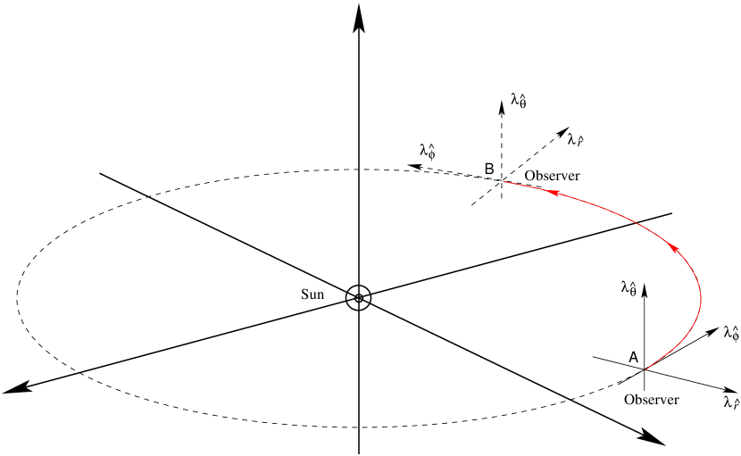
Figure 9: The spatial axes of a phase-locked tetrad are such that one is constantly lying in the Sun-observer direction, one is always tangent to the circular path of the observer around the Sun and the third axes is orthogonal to the orbital plane. The figure shows how these axes change when the observer moves from A to B along the fraction of the orbit represented with solid line.

Table 4: Difference (in $\mu$arcsec) between the parallax $p^{*}_{e}$ calculated from the exact Schwarzschild model and that reconstructed using our $(v/c)^{2}$ model ($p^{*}_{a}$). The first column reports the exact distance in parsec, the remaining four give $(p^{*}_{e}-p^{*}_{a})$ as obtained for each of the corresponding $\varepsilon_{r_{c}}$, the level of accuracy for the impact parameter $r_{c}$ expressed in meters.

$r^{*}_{e}~{}($pc$)$	$(p^{*}_{e}-p^{*}_{a})~{}(\mu$arcsec$)$
	$\varepsilon_{r_{c}}=4.8$	$\varepsilon_{r_{c}}=9.6\cdot 10^{-2}$	$\varepsilon_{r_{c}}=1.9\cdot 10^{-3}$	$\varepsilon_{r_{c}}=4\cdot 10^{-5}$
$1$	$-262.2$	$-12.5$	$-17.8$	$-17.8$
$10$	$\phantom{-}124.6$	$-19.1$	$-17.8$	$-17.8$
$100$	$\phantom{-}150.9$	$-23.1$	$-17.8$	$-17.8$
$1000$	$\phantom{-}229.1$	$-20.6$	$-17.7$	$-17.8$
$10000$	$\phantom{-}\phantom{0}85.6$	$-12.8$	$-17.8$	$-17.8$

7.3 Stellar distances test: comparison with a Schwarzschild model

Recently we developed a Schwarzschild model for astrometric observations (Vecchiato, 1996; de Felice et al., 1998). In that model we express the components of the vector $k^{i}$ tangent to a null geodesic relative to the spatial axes $\hat{r}$, $\hat{\theta}$ and $\hat{\phi}$ of a phase-locked tetrad adapted to an observer on a circular orbit around the Sun (Figure 9), namely (de Felice and Usseglio-Tomasset, 1992)

$$\textbf{e}_{\hat{r}}\equiv\cos\Theta_{(\hat{r},k)} = \pm\frac{\sqrt{\left(1-\frac{2M_{\odot}}{r_{\rm{o}}}\right)^{-1}-\frac{\Lambda^{2}}{r_{\rm{o}}^{2}}}}{\left(1-\omega\lambda\right)\sqrt{1-\frac{3M_{\odot}}{r_{\rm{o}}}}}$$ (61)

$$\textbf{e}_{\hat{\theta}}\equiv\cos\Theta_{(\hat{\theta},k)} = \pm\frac{\frac{1}{r_{\rm{o}}}\sqrt{\Lambda^{2}-\lambda^{2}}}{\left(1-\omega\lambda\right)\sqrt{1-\frac{3M_{\odot}}{r_{\rm{o}}}}}$$ (62)

$$\textbf{e}_{\hat{\phi}}\equiv\cos\Theta_{(\hat{\phi},k)} = \frac{\sqrt{1-\frac{2M_{\odot}}{r_{\rm{o}}}}\left[\lambda-\frac{\omega r_{\rm{o}}^{2}}{1-\frac{2M}{r_{\rm{o}}}}\right]}{r_{\rm{o}}\left(1-\omega\lambda\right)}.$$ (63)

Here $r_{\rm{o}}$ is the distance of the observer from the Sun, $\omega$ is the coordinate angular velocity of the observer, while $\Lambda$ and $\lambda$ are two constants of motion of the null geodesic. The constants of motion $\lambda$ and $\Lambda$ can be expressed as functions of the impact parameter of the light geodesic with respect to the Sun ($r_{c}$) and of the angular Schwarzschild coordinates of the star $(\theta,\phi)$. Finally, $r_{c}$ can be implicitly expressed as a function of the complete set of Schwarzschild coordinates of the star $(r,\theta,\phi)$. This means that, given the position of a star and of an observer (in Schwarzschild coordinates), we are able to derive the Cartesian components of the tangent to the null geodesic at the position of the observer by means of an almost completely analytical procedure. These components allow us to define the observables according to Eq.(21).

In the present model, we can reproduce the same physical situation and the same observables by taking $h_{\alpha\beta}$ as the approximation to the Schwarzschild metric and by adopting the tetrad, defined by Eqs.(35)–(38), of an observer on a circular orbit. Hence we can use those observables and the position of the observer as the boundary conditions needed to integrate backwards the set of differential equations (19). It was this complementarity of the two algorithms that was exploited for our test.

We start by giving the “true” position of a star $(r^{*},\theta^{*},\phi^{*})$ and two symmetric observers (with respect to the Sun) $(r_{1},\theta_{1},\phi_{1})$ and $(r_{2},\theta_{2},\phi_{2})$ in the “Schwarzschild model”, from which we calculate the tetraedal components of the local light directions for both observers using Eqs.(61)–(63). Let’s call those components $(\textbf{e}_{r_{1}},\textbf{e}_{\theta_{1}},\textbf{e}_{\phi_{1}})$ and $(\textbf{e}_{r_{2}},\textbf{e}_{\theta_{2}},\textbf{e}_{\phi_{2}})$. Note that $(r_{1},\theta_{1},\phi_{1})$ and $(\textbf{e}_{r_{1}},\textbf{e}_{\theta_{1}},\textbf{e}_{\phi_{1}})$ represent the boundary conditions needed in our model to integrate the light trajectory for the first observer, and analogously $(r_{2},\theta_{2},\phi_{2})$ and $(\textbf{e}_{r_{2}},\textbf{e}_{\theta_{2}},\textbf{e}_{\phi_{2}})$ are the boundary conditions for the second observer.

The point of intersection of the two paths obtained in this way should be the position of the star at $(r^{*},\theta^{*},\phi^{*})$; however we expect to find slightly different coordinates $(r^{*}_{a},\theta^{*}_{a},\phi^{*}_{a})$. Indeed, there are two reasons for this difference: the approximation of our perturbative model which is up to $(v/c)^{2}$, and possible numerical errors. The latter should always be maintained below the level of the intrinsic approximation.

In this test we have taken the two observers at opposite positions on the orbit of the Earth around the Sun (i.e. $r_{1}=r_{2}=r_{\rm{o}}$, $\theta_{1}=\theta_{2}=\pi/2$ and $\phi_{2}=\phi_{1}+\pi$). The stars are also on the orbital plane ($\theta^{*}=\pi/2$) in such a way the two observers are symmetrically placed with respect to the Sun-star direction ($\phi^{*}=(\phi_{1}+\phi_{2})/2$). Their distances ($r^{*}$) range from $1$ pc to $10$ kpc.

With this configuration it is easy to calculate the parallax of a star as $p^{*}=1/r^{*}$ rad (the distances being in AU), and so it is equally easy to determine the numerical accuracy of the position in terms of angles by simply subtracting the parallax $p^{*}_{e}$ of the exact model from the approximate one, $p^{*}_{a}$, reconstructed from the numerical integrations described above.

The results in Table 4, show that there is an accuracy floor at about $18~{}\mu$arcsec, as one could expect given the intrinsic level of approximation of the model. This table also shows that an accuracy on the determination of $r_{c}$ to $\sim 10^{-3}$ m at least, is needed to reach the theoretical floor for $(p^{*}_{e}-p^{*}_{a})$. We stress that in our case, where $r_{c}\simeq r_{0}\simeq 1.5\cdot 10^{11}~{}$m, this means that the numerical accuracy needed is $\varepsilon_{r_{c}}/r_{c}\sim 10^{-14}$, pushing to the edge the typical accuracy for a standard double precision number; however to this level the numerical contribution to the error is contained to the $0.1~{}\mu$arcsec level.

Figure 10: The geometrical configuration of the deflection test with more than one body is such that all the planets are aligned behind the Sun and along the line joining the Sun with the observer.

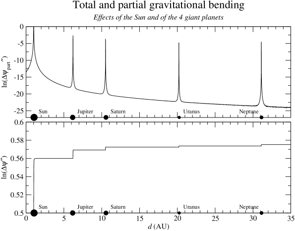
Figure 11: The upper plot shows the natural logarithm of the partial deflection $\Delta\psi_{\rm{part}}$ (expressed in arcseconds) of the light ray due to the Sun and the four major planets of the Solar System, while the other gives the total deflection. Both are plotted against the approximate distance $d$ from the observer in Astronomical Units. All the bodies considered are drawn as circles in their approximate locations along the $x$-axis.

8 N-body tests

The tests described in section 7 consider the Sun as the unique source of gravity. This is because in that section we wanted to compare our $(v/c)^{2}$ model with an exact one (or at least with a model which was already tested at the level of accuracy we require) and the obvious choice was the Schwarzschild model.

However, our model has been built to include an arbitrary number of gravity sources. We shall then subject our model with more than one gravitating body to similar tests to see whether in this case the results are consistent with expectations. This will also serve as the proper testing ground for our forthcoming $(v/c)^{3}$ model and whatever others would be available. Indeed, to the best of our knowledge, we do not know of any extensive numerical testing for multi-body relativistic models.

8.1 Deflection due to a variable number of aligned bodies

In this test we have calculated the total deflection due to the Sun plus a variable number of planets. The geometry is depicted in Figure 10; here the planets are aligned behind the Sun with respect to the observer and the light ray was assumed to be grazing the solar limb. The results are reported in Table 5 and in Figure 11.

The first row of the table provides the total deflection in four different cases: the first one gives the result for the Sun plus Jupiter, the second one for the Sun, Jupiter and Saturn, and so on.

Table 5: Results for the multi-body deflection test. All the numbers are expressed in arcseconds. The first row gives the total deflection due to the gravitational pull of the Sun, plus that of the planet indicated in the corresponding column heading, and plus that of all the other planets on its left. The value of the deflection in the last row, $\Delta\psi_{\astrosun}$, is for a light ray grazing the limb of the Sun, i.e. where the distance of closest approach to the center of the Sun is $r_{\mathrm{c}}=R_{\astrosun}=696\,000$ km.

	Jupiter (♃)	Saturn (♄)	Uranus (⛢)	Neptune (♆)
$\Delta\psi_{i}$	$1.7509921$	$1.7510398$	$1.7510436$	$1.7510465$
$\Delta\equiv\Delta\psi_{\astrosun}-\Delta\psi_{i}$	$0.0002699$	$0.0003176$	$0.0003214$	$0.0003243$
$\Delta_{\mathrm{schw}}$	$0.0002695$	$0.0003172$	$0.0003210$	$0.0003239$
$\Delta-\Delta_{\mathrm{schw}}$	$0.0000004$	$0.0000004$	$0.0000004$	$0.0000004$
$\Delta\psi_{\astrosun}=1.7507222$

The second row shows the differences between the deflection due to the Sun (i.e. the value $\Delta\psi_{\astrosun}$) and the amount of total deflection immediately above. This difference gives the deflection due to the planets alone.

The same effect can be approximately estimated calculating the light deflection due to each planet, with the analytical formula for the Schwarzschild solution, and summing them up. This is what is represented in the third row. Finally the fourth row simply reports the differences among the values in second row and those in third.

We stress here that the predictions contained in the third row are not well justified from a theoretical point of view. However they can be considered reasonably close to reality; hence this and the following tests just tell us that our model behaves “well” with respect to a reasonable (but not exact) model under the same physical situation.

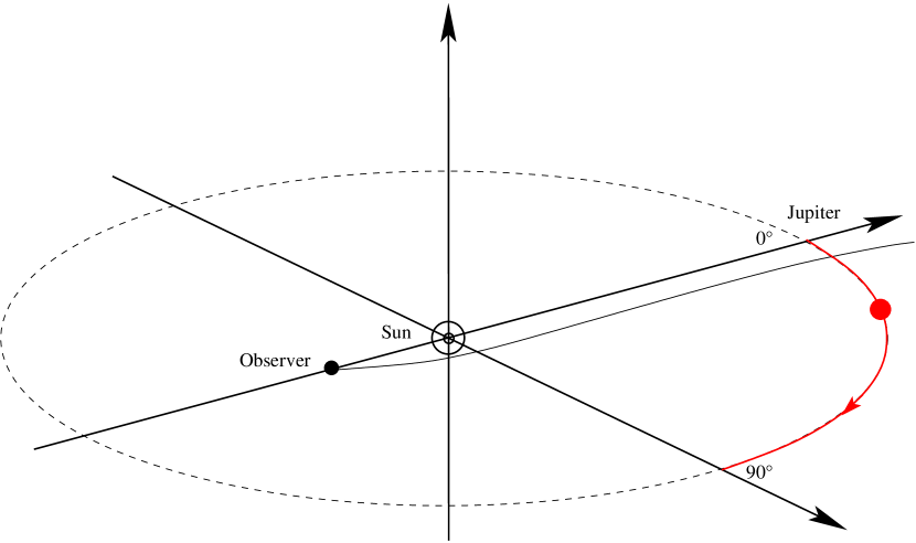
Figure 12: The total deflection due to the Sun and Jupiter was calculated varying the position of Jupiter along its orbit.

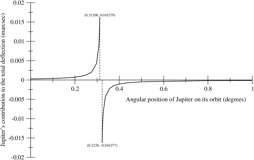
Figure 13: When Jupiter is aligned with the Sun and the observer its position on the orbit is $\alpha=0^{\circ}$. Its contribution to the total deflection increases approximately to $16.28$ mas for $\alpha\simeq 0^{\circ}\!\!.31208$, where the light path grazes both the Sun and the planet leaving them on the same side. For $\alpha\simeq 0^{\circ}\!\!.3226$ the light ray still grazes both of them, but passing in the middle, so that Jupiter’s contribution subtracts to the total deflection. With Jupiter in the range $0^{\circ}\!\!.31208<\alpha<0^{\circ}\!\!.3226$ the photons are stopped by the planet.

Table 6: Results for the test of section 8.2. The angular positions of Jupiter are in degrees and the deflections in arcseconds.

Angle	$\Delta\psi_{\mathrm{tot}}$	$\Delta\psi_{\jupiter}$
0.0000000	1.7509921	0.0002699
0.0355333	1.7510261	0.0003039
0.0794550	1.7510823	0.0003601
0.1123663	1.7511401	0.0004179
0.1376200	1.7511988	0.0004766
0.1589100	1.7512629	0.0005407
0.1776667	1.7513355	0.0006133
0.1946242	1.7514202	0.0006980
0.2247327	1.7516472	0.0009250
0.2512588	1.7520185	0.0012963
0.2752403	1.7527570	0.0020348
0.2972935	1.7549956	0.0042734
0.3077281	1.7596352	0.0089130
0.3097728	1.7620437	0.0113215
0.3118041	1.7661978	0.0154756
0.3120065	1.7667852	0.0160630
0.3120672	1.7669702	0.0162480
0.3120773	1.7670014	0.0162792
0.3226012	1.7344451	-0.0162771
0.3226110	1.7344754	-0.0162468
0.3227480	1.7348868	-0.0158354
0.3229435	1.7354393	-0.0152829
0.3237245	1.7373081	-0.0134141
0.3256688	1.7404386	-0.0102836
0.3276016	1.7423752	-0.0083470
0.3370993	1.7463871	-0.0043351
0.3553339	1.7484676	-0.0022546
0.3726774	1.7491742	-0.0015480
0.3892489	1.7495309	-0.0011913
0.4051432	1.7497466	-0.0009756
0.4204370	1.7498130	-0.0009092
0.4351937	1.7499953	-0.0007269
0.5025188	1.7502596	-0.0004626
0.7945559	1.7505427	-0.0001795
0.9401342	1.7505846	-0.0001376
1.1236807	1.7506159	-0.0001063
1.3762332	1.7506413	-0.0000809
1.5891499	1.7506548	-0.0000674
1.9463344	1.7506696	-0.0000526
2.2474695	1.7506778	-0.0000444
2.5127875	1.7506832	-0.0000390
3.5539031	1.7506957	-0.0000265
7.9518754	1.7507110	-0.0000112
11.2547126	1.7507143	-0.0000079
15.9423686	1.7507167	-0.0000055
19.5572137	1.7507177	-0.0000045
30.0733476	1.7507193	-0.0000029
39.7151372	1.7507200	-0.0000022
54.7655820	1.7507206	-0.0000016
67.3801351	1.7507209	-0.0000013
78.9125108	1.7507211	-0.0000011
90.0000000	1.7507213	-0.0000009

Table 7: The distance of maximum approach of the light ray to Jupiter ($r_{\mathrm{min}}$) is calculated in the two extremal cases in which the photons pass nearby the limb of the planet. It is always slightly more than the planet’s actual radius $R_{\jupiter}=71398$ km (Murray and Dermott, 1999).

Row	$r_{\mathrm{min}}$	$\Delta\psi_{\jupiter}$
18	71461 km	$\phantom{-}0^{\prime\prime}\!\!.0162792$
19	71474 km	$-0^{\prime\prime}\!\!.0162771$

8.2 Deflection of two bodies with variable relative position

In this test we considered only two bodies, the Sun and Jupiter, and calculated the total light deflection experienced by a light ray grazing the solar limb and positioning Jupiter in several different places along its orbit. In particular, the planet’s position varied in a range of $90$ degrees, from conjunction to quadrature (Figure 12).

The results (Table 6 and Figure 13) show that the contribution of Jupiter, as it should be, adds to that of the Sun when the two masses are both “on the same side” with respect to the light path; their their influences subtract when the light passes between the bodies. Moreover, when the light ray grazes the Jovian limb (rows number 18 and 19 of Table 6), the contribution to the total deflection due to the planet approaches the predicted theoretical value of $16.28$ marcsec (de Felice et al., 2000; Klioner, 2000) as shown in Table 7.

Finally, it is also worth noting that the amount of Jupiter’s contribution to the total deflection is of the order of $1~{}\mu$arcsec when the planet is $90$ degrees far from the light path, again in very good agreement with the theoretical predictions (Klioner, 2000).

Table 8:

	☉	☉+♃	☉+♃+♄	☉+♃+♄+⛢	☉+♃+♄+⛢+♆
distance $\sim 1$ pc
$d~{}($AU$)$	206261.338	206259.698	206259.216	206259.142	206259.054
$p_{i}~{}(^{\prime\prime})$	1.00001775	1.00002571	1.00002804	1.00002840	1.00002883
$p_{i}-p_{\astrosun}~{}(\mu$arcsec$)$	$\cdots$	-7.95	-10.29	-10.65	-11.07
$\Delta\psi_{i}~{}(\mu$arcsec$)$	$\cdots$	-8.00	-10.30	-10.60	-11.10
distance $\sim 10$ pc
$d~{}($AU$)$	2062283.55	2062120.14	2062072.27	2062064.94	2062056.3
$p_{i}~{}(^{\prime\prime})$	0.10001777	0.10002569	0.10002802	0.10002837	0.10002879
$p_{i}-p_{\astrosun}~{}(\mu$arcsec$)$	$\cdots$	-7.93	-10.25	-10.60	-11.02
$\Delta\psi_{i}~{}(\mu$arcsec$)$	$\cdots$	-8.00	-10.30	-10.60	-11.00
distance $\sim 100$ pc
$d~{}($AU$)$	20589921.6	20573645.4	20568881.5	20568152.5	20567292.3
$p_{i}~{}(^{\prime\prime})$	0.01001777	0.01002569	0.01002801	0.01002837	0.01002879
$p_{i}-p_{\astrosun}~{}(\mu$arcsec$)$	$\cdots$	-7.93	-10.25	-10.60	-11.02
$\Delta\psi_{i}~{}(\mu$arcsec$)$	$\cdots$	-7.99	-10.30	-10.60	-11.00
distance $\sim 1000$ pc
$d~{}($AU$)$	202664764	201098829	200644596	200575248	200493473
$p_{i}~{}(^{\prime\prime})$	0.00101776	0.00102569	0.00102801	0.00102837	0.00102879
$p_{i}-p_{\astrosun}~{}(\mu$arcsec$)$	$\cdots$	-7.93	-10.25	-10.60	-11.02
$\Delta\psi_{i}~{}(\mu$arcsec$)$	$\cdots$	-7.99	-10.30	-10.60	-11.00
distance $\sim 10000$ pc
$d~{}($AU$)$	1751489760	1641052370	1611285280	1609051510	1603803810
$p_{i}~{}(^{\prime\prime})$	0.00011777	0.00012569	0.00012801	0.00012819	0.00012861
$p_{i}-p_{\astrosun}~{}(\mu$arcsec$)$	$\cdots$	-7.93	-10.25	-10.42	-10.84
$\Delta\psi_{i}~{}(\mu$arcsec$)$	$\cdots$	-7.99	-10.30	-10.60	-11.00

8.3 Stellar distances revisited: effect of many bodies

As a final test, we have repeated the experiment of section 7.3, but with an increasing number of aligned planets as in section 8.1 (the sequence of planets was kept the same). However, unlike the previous case, in this test we cannot compare our model with any other, so this is in fact another test of self-consistency for the $(v/c)^{2}$ model. The sense of this statement will be clarified below.

Figure 14: The same initial conditions (i.e. viewing directions) should result in a decreased distance of the star when other planets are added.

We consider the same boundary conditions as those used for the test with the Schwarzschild model. These were unchanged as we added Jupiter, Saturn and the other planets.

Therefore, the expectation was the the distance to a star decreased as we added more planets (and the corresponding parallax increased) because of the increased total deflection (Figure 14).

The results are reported in Table 8. Stellar distances, as before, ranged from 1 pc to 10 kpc. The first row in each set of 4 is the derived distance, $d$, in AU (i.e. that obtained by the intersection of the two geodesics), the second is the corresponding parallax $p=206265/d$ arcsec. The third row contains the difference between $p_{\astrosun}$ and the parallax of the corresponding column. For instance, in the case of Jupiter, the value is $p_{\astrosun}-p_{\jupiter}\equiv\Delta p_{\jupiter}$. Finally, the fourth row provides the contribution $\Delta\psi_{i}$, ($i=\jupiter,\saturn,\uranus,\neptune$) of the planets to the total deflection. This contribution is calculated independently, following the method used in section 8.1.

The self-consistency of the model assures that these last two values coincide up to numerical errors.

The results show that, as we add more planets, the distances decrease confirming our qualitative expectations. Moreover, the numerical residuals are $\Delta p_{i}-\Delta\psi_{i}\lesssim 10^{-1}~{}\mu$arcsec ($i=\jupiter,\saturn,\uranus,\neptune$), and this again is compatible with our accuracy for double precision numbers.

9 Conclusions

We have developed a general relativistic astrometric n-body model capable of following a light ray all the way from the emitting star to an observer (satellite) orbiting around the Sun.

This model has an intrinsic accuracy of $\sim 0.1$ milliarcsecond ($(v/c)^{2}$) and its computer implementation was validated via a thorough test campaign that proved: a) the self-consistency of the model; b) that the amount of light deflection, in the case of a spherical, non-rotating, single-body metric, coincides with that produced by an analytical solution; c) that, under the same assumptions, our model is able to reconstruct stellar distances; d) that in the case of a multi-body configuration, for which we don’t have any exact or even well-founded analytical approximation, the outcomes for the light deflection and the reconstruction of stellar distances are consistent with the results from semi-quantitative derivations.

Finally, this model will be the natural test-bed for the more advanced astrometric model, accurate to $(v/c)^{3}$, which will be presented in a forthcoming article.

Appendix A Mathematical description of the mapping procedure

Here we describe rigorously the mathematical procedure used to obtain the spatial projection of the light ray on the slice $S(\tau_{0})$. The null geodesic crosses each slice $S(\tau)$ at a point with coordinates $\xi^{i}=\xi^{i}(\lambda(\tau))$; but this point also belongs to the unique normal to the slice $S(\tau)$, crossing it with a value of the parameter $\sigma=\sigma(\xi^{i}(\lambda),\,\tau)\equiv\sigma_{\xi^{i}(\lambda)}(\tau)$. (Figure 2).

Let us now define the one-parameter local diffeomorphism:

$$\phi_{\Delta\sigma}\equiv\phi_{(\sigma_{\xi^{i}(\lambda)}(\tau_{0})-\sigma_{\xi^{i}(\lambda)}(\tau))}\,:\,\mit\Upsilon\cap S(\tau)\to S(\tau_{0})$$ (A1)

which maps each point of the null geodesic $\mit\Upsilon$ to the point on the slice $S(\tau_{0})$ which one gets to by moving along the unique normal through the point $\mit\Upsilon(\lambda)\cap S(\tau)$, by a parameter distance $\Delta\sigma=\sigma_{\xi^{i}(\lambda)}(\tau_{0})-\sigma_{\xi^{i}(\lambda)}(\tau)$ (Figure 2). Since the spatial coordinates $\xi^{i}$ are Lie-transported along the normals to the slices, then the points in $S(\tau_{0})$, which are images of those on the null geodesic under $\phi_{\Delta\sigma}$, have coordinates $(\phi_{\Delta\sigma}(\mit\Upsilon(\lambda)\cap S(\tau)))^{i}=\xi^{i}$. The curve in $S(\tau_{0})$ which is the image of $\mit\Upsilon$ under $\phi_{\Delta\sigma}$, is:

$$\bar{\mit\Upsilon}\equiv\phi_{\Delta\sigma}\circ\mit\Upsilon;$$ (A2)

it has tangent vector:

$$\dot{\bar{\mit\Upsilon}}^{\alpha}=\dot{\Big{(}\phi_{\Delta\sigma}^{*}\circ k\Big{)}}^{\alpha}=\frac{\partial\xi^{\alpha}(\sigma(\tau_{0}))}{\partial\xi^{\beta}(\sigma(\tau))}k^{\beta}\equiv\ell^{\alpha}.$$ (A3)

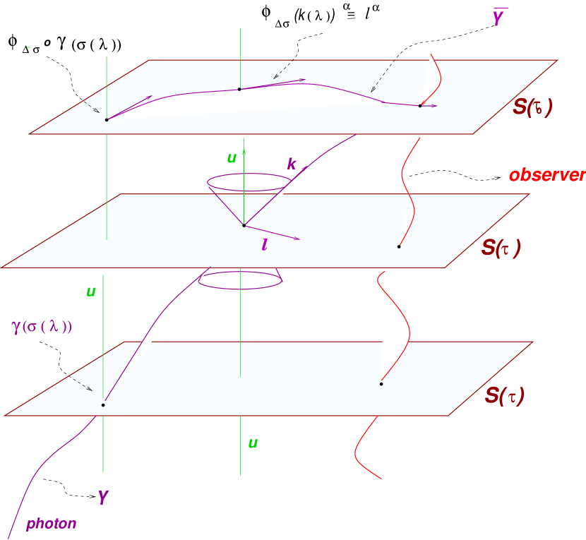
Figure 15: The curve $\bar{\mit\Upsilon}$ will be the image of the null geodesic $\mit\Upsilon_{k}$ under the diffeomorphism $\phi_{\Delta\sigma}$.

The map (A1) acts on a 4-dimensional manifold with images in a 3-dimensional one hence the coordinates of the target points ($\mit\Upsilon\cap S(\tau)$) and those of the image points on $S(\tau_{0})$ are respectively:

$$\xi^{\alpha}(\sigma(\tau)) = \tau\delta^{\alpha}_{0}+\xi^{i}(\sigma(\tau))\delta^{\alpha}_{i}$$

$$\xi^{\alpha}(\sigma(\tau_{0})) = \xi^{\alpha}(\sigma(\tau))-\tau\delta^{\alpha}_{0}.$$

From this and (A2) it follows that (Figure 15).

$$\ell^{\alpha}=\tilde{\gamma}^{\alpha}{}_{\beta}k^{\beta}\,,$$ (A4)

hence the curve $\bar{\mit\Upsilon}$ is the spatial projection of the null geodesic on the slice $S(\tau_{0})$ at the time of observation.

Appendix B Explicit expression for the tetrad components

The following expressions represent the coordinate components of each tetrad vector $\lambda_{\hat{a}}$ (a= 1, 2, 3) with respect the coordinate basis $\bm{\partial_{\alpha}}$ ($\alpha=0,x,y,z$) when the observer moves on the orbit which has general barycentric component $X_{s}$, $Y_{s}$, $Z_{s}$ (to be specified):

$$T_{s} = 1$$

$$T_{1} = 0$$

$$X_{1} = \mp\frac{Y_{s}\sqrt{g_{yy}}}{\sqrt{g_{xx}}\sqrt{g_{xx}X_{s}^{2}+g_{yy}Y_{s}^{2}}}$$

$$Y_{1} = \pm\frac{X_{s}\sqrt{g_{xx}}}{\sqrt{g_{yy}}\sqrt{g_{xx}X_{s}^{2}+g_{yy}Y_{s}^{2}}}$$

$$Z_{1} = 0$$

$$T_{2} = \mp\frac{\sqrt{(g_{xx}X_{s}^{2}+g_{yy}Y_{s}^{2})/(g_{00}+g_{zz}Z_{s}^{2})}}{\sqrt{g_{00}+g_{xx}X_{s}^{2}+g_{yy}Y_{s}^{2}+g_{zz}Z_{s}^{2}}}$$

$$X_{2} = \pm\frac{X_{s}\sqrt{(g_{00}+g_{zz}Z_{s}^{2})/(g_{xx}X_{s}^{2}+g_{yy}Y_{s}^{2})}}{\sqrt{g_{00}+g_{xx}X_{s}^{2}+g_{yy}Y_{s}^{2}+g_{zz}Z_{s}^{2}}}$$

$$Y_{2} = \pm\frac{Y_{s}\sqrt{(g_{00}+g_{zz}Z_{s}^{2})/(g_{xx}X_{s}^{2}+g_{yy}Y_{s}^{2})}}{\sqrt{g_{00}+g_{xx}X_{s}^{2}+g_{yy}Y_{s}^{2}+g_{zz}Z_{s}^{2}}}$$

$$Z_{2} = \mp\frac{Z_{s}\sqrt{(g_{xx}X_{s}^{2}+g_{yy}Y_{s}^{2})/(g_{00}+g_{zz}Z_{s}^{2})}}{\sqrt{g_{00}+g_{xx}X_{s}^{2}+g_{yy}Y_{s}^{2}+g_{zz}Z_{s}^{2}}}$$

$$T_{3} = \mp\frac{Z_{s}\sqrt{g_{zz}}}{\sqrt{g_{00}}\sqrt{g_{00}+g_{zz}Z_{s}^{2}}}$$

$$X_{3} = 0$$

$$Y_{3} = 0$$

$$Z_{3} = \pm\frac{\sqrt{g_{00}}}{\sqrt{g_{zz}}\sqrt{g_{00}+g_{zz}Z_{s}^{2}}}.$$

References

- Ashby and Bertotti (1986) N. Ashby and B. Bertotti. Relativistic effects in local inertial frames. Phys. Rev. D, 34:2246–2259, October 1986.
- Bertotti and Grishchuk (1990) B. Bertotti and L. P. Grishchuk. The strong equivalence principle . Class. Quantum Grav., 7:1733–1745, October 1990.
- Brumberg (1991) V. A. Brumberg. Essential Relativistic Celestial Mechanics. Adam Hilger, Bristol, 1991.
- Brumberg and Kopeikin (1989) V. A. Brumberg and S. M. Kopeikin. Relativistic Reference Systems and Motion of Test Bodies in the Vicinity of the Earth. Nuovo Cimento B, 103:63–98, 1989.
- Damour et al. (2002a) T. Damour, F. Piazza, and G. Veneziano. Runaway Dilaton and Equivalence Principle Violations. Phys. Rev. Lett., 89(8):81601, August 2002a.
- Damour et al. (2002b) T. Damour, F. Piazza, and G. Veneziano. Violations of the equivalence principle in a dilaton-runaway scenario. Phys. Rev. D, 66:46007, August 2002b.
- Damour et al. (1991) T. Damour, M. Soffel, and C. Xu. General-relativistic celestial mechanics. I. Method and definition of reference systems. Phys. Rev. D, 43:3273–3307, May 1991.
- Damour et al. (1992) T. Damour, M. Soffel, and C. Xu. General-relativistic celestial mechanics. II. Translational equations of motion. Phys. Rev. D, 45:1017–1044, February 1992.
- Damour et al. (1993) T. Damour, M. Soffel, and C. Xu. General-relativistic celestial mechanics. III. Rotational equations of motion. Phys. Rev. D, 47:3124–3135, April 1993.
- Damour et al. (1994) T. Damour, M. Soffel, and C. Xu. General-relativistic celestial mechanics. IV. Theory of satellite motion. Phys. Rev. D, 49:618–635, January 1994.
- de Felice et al. (2001) F. de Felice, B. Bucciarelli, M. G. Lattanzi, and A. Vecchiato. General relativistic satellite astrometry. II. Modeling parallax and proper motion. Astron. Astrophys., 373:336–344, July 2001.
- de Felice and Clarke (1990) F. de Felice and C. J. S. Clarke. Relativity on curved manifolds. Cambridge University Press, 1990.
- de Felice et al. (1998) F. de Felice, M. G. Lattanzi, A. Vecchiato, and P. L. Bernacca. General relativistic satellite astrometry. I. A non-perturbative approach to data reduction. Astron. Astrophys., 332:1133–1141, April 1998.
- de Felice and Usseglio-Tomasset (1992) F. de Felice and S. Usseglio-Tomasset. Circular Orbits and Relative Strains in Schwarzschild Space-Time. Gen. Relativ. Gravit., 24:1091, 1992.
- de Felice et al. (2000) F. de Felice, A. Vecchiato, B. Bucciarelli, M. Lattanzi, and M. Crosta. General Relativistic Models for a GAIA-like Astrometry Mission. In IAU Colloq. 180: Towards Models and Constants for Sub-Microarcsecond Astrometry, page 314, 2000.
- Dominik and Sahu (2000) M. Dominik and K. C. Sahu. Astrometric Microlensing of Stars. Astrophys. J., 534:213–226, May 2000.
- Epstein and Shapiro (1980) R. Epstein and I. I. Shapiro. Post-post-Newtonian deflection of light by the Sun. Phys. Rev. D, 22:2947–2949, December 1980.
- Everhart (1985) E. Everhart. An Efficient Integrator that Uses Gauss-Radau Spacings. In A. Carusi and G. B. Valsecchi, editors, IAU Colloq. 83: Dynamics of comets: their origin and evolution, volume 115 of Astrophysics and Space Science Library, pages 185–202. D. Reidel Publishing Company, 1985.
- Fomalont and Kopeikin (2003) E. B. Fomalont and S. M. Kopeikin. The Measurement of the Light Deflection from Jupiter: Experimental Results. Astrophys. J., 598:704–711, November 2003.
- Klioner (2000) S. A. Klioner. Relativity in Modern Astrometry and Celestial Mechanics - Overview. In IAU Colloq. 180: Towards Models and Constants for Sub-Microarcsecond Astrometry, page 265, 2000.
- Klioner (2003) S. A. Klioner. A Practical Relativistic Model for Microarcsecond Astrometry in Space. Astron. J., 125:1580–1597, March 2003.
- Klioner and Kopeikin (1992) S. A. Klioner and S. M. Kopeikin. Microarcsecond astrometry in space - Relativistic effects and reduction of observations. Astron. J., 104:897–914, August 1992.
- Klioner and Voinov (1993) S. A. Klioner and A. V. Voinov. Relativistic theory of astronomical reference systems in closed form. Phys. Rev. D, 48:1451–1461, August 1993.
- Kopeikin (2001) S. M. Kopeikin. Testing the Relativistic Effect of the Propagation of Gravity by Very Long Baseline Interferometry. Astrophys. J. Lett., 556:L1–L5, July 2001.
- Kopeikin and Mashhoon (2002) S. M. Kopeikin and B. Mashhoon. Gravitomagnetic effects in the propagation of electromagnetic waves in variable gravitational fields of arbitrary-moving and spinning bodies. Phys. Rev. D, 65:64025, March 2002.
- Kopeikin and Schäfer (1999) S. M. Kopeikin and G. Schäfer. Lorentz covariant theory of light propagation in gravitational fields of arbitrary-moving bodies. Phys. Rev. D, 60:124002, December 1999.
- Marr (2003) J. C. Marr. Space interferometry mission (SIM): overview and current status. In Interferometry in Space. Edited by Shao, Michael. Proceedings of the SPIE, Volume 4852, pp. 1-15 (2003)., pages 1–15, February 2003.
- Misner et al. (1973) C. W. Misner, K. S. Thorne, and J. A. Wheeler. Gravitation. San Francisco: W.H. Freeman and Co., 1973.
- Murray and Dermott (1999) C. D. Murray and S. F. Dermott. Solar System Dynamics. Cambridge University Press, 1999.
- Perryman (2003) M. A. C. Perryman. The GAIA mission. In U. Munari, editor, GAIA Spectroscopy, Science and Technology, volume 298 of ASP Conf. Ser., pages 3–12, 2003. Proceedings of the Monte Rosa International Conference “GAIA Spectroscopy, Science and Technology”, Sept. 9-12 2002, Gressoney St. Jean (Aosta), Italy.
- Perryman et al. (2001) M. A. C. Perryman, K. S. de Boer, G. Gilmore, E. Høg, M. G. Lattanzi, L. Lindegren, X. Luri, F. Mignard, O. Pace, and P. T. de Zeeuw. GAIA: Composition, formation and evolution of the Galaxy. Astron. Astrophys., 369:339–363, April 2001.
- Sazhin et al. (1998) M. V. Sazhin, V. E. Zharov, A. V. Volynkin, and T. A. Kalinina. Microarcsecond instability of the celestial reference frame. Mon. Not. R. Astron. Soc., 300:287–291, October 1998.
- Shao (1998) M. Shao. SIM: the space interferometry mission. In Proc. SPIE Vol. 3350, p. 536-540, Astronomical Interferometry, Robert D. Reasenberg; Ed., pages 536–540, July 1998.
- Soffel (2000) M. Soffel. Report of the Working Group “Relativity for Celestial Mechanics and Astrometry”. In IAU Colloq. 180: Towards Models and Constants for Sub-Microarcsecond Astrometry, page 283, 2000.
- Vecchiato (1996) A. Vecchiato. Astrometria relativistica. Applicazioni al progetto GAIA. Thesis (tesi di laurea), University of Padova — Dept. of Physics, June 1996. In italian.