A relativistic helical jet in the $\gamma$-ray AGN 1156+295

We present the results of a number of high resolution radio observations of the AGN 1156+295. These include multi-epoch and multi-frequency VLBI, VSOP, MERLIN and VLA observations made over a period of 50 months. The 5 GHz MERLIN images trace a straight jet extending to $\sim 2\arcsec$ at ${\rm P.A.}\sim-18\degr$. Extended low brightness emission was detected in the MERLIN observation at 1.6 GHz and the VLA observation at 8.5 GHz with a bend of $\sim 90\degr$ at the end of the 2 arcsecond jet. A region of similar diffuse emission is also seen about 2 arcseconds south of the radio core. The VLBI images of the blazar reveal a core-jet structure with an oscillating jet on a milli-arcsecond (mas) scale which aligns with the arcsecond jet at a distance of several tens of milli-arcseconds from the core. This probably indicates that the orientation of the jet structure is close to the line of sight, with the northern jet being relativistically beamed toward us. In this scenario the diffuse emission to the north and south is not beamed and appears symmetrical. For the northern jet at the mas scale, proper motions of $13.7\pm 3.5,10.6\pm 2.8$, and $11.8\pm 2.8\;c$ are measured in three distinct components of the jet ($q_{0}=0.5$, $H_{0}=65\leavevmode\nobreak\$km s^-1Mpc^-1 are used through out this paper). Highly polarised emission is detected on VLBI scales in the region in which the jet bends sharply to the north-west. The spectral index distribution of the source shows that the strongest compact component has a flat spectrum, and the extended jet has a steep spectrum. A helical trajectory along the surface of a cone was proposed based on the conservation laws for kinetic energy and momentum to explain the observed phenomena, which is in a good agreement with the observed results on scales of 1 mas to 1 arcsec.

1 Introduction

The AGN 1156+295 is extremely variable over a broad range of the electromagnetic spectrum, from radio waves to $\gamma$-rays. At a redshift of $z=0.729$ (Véron-Cetty & Véron (1998)), it has been classified as both a Highly Polarised Quasar (HPQ) and an Optically Violent Variable (OVV) source (Wills et al. (1983), 1992, Glassgold et al. (1983)). In its active phase, the source shows fluctuations at optical wavelengths with an amplitude of $\sim 5-7\%$ on a time scale of 0.5 hour (Wills et al. (1983)). There are also large and rapid changes of the optical linear polarization, with the percentage of polarised flux density changing between $1-29\%$ (Wills et al. (1992)). It is one of the class of radio sources detected by EGRET (Energetic Gamma Ray Experiment Telescope) on the Compton Gamma Ray Observatory. While quiescent $\gamma$-ray emission remains undetected in the source, three strong flares ($\sim 3.9\times 10^{-10}$ Jy) were detected by EGRET at energies $>100$ MeV during the period from 1992 to 1996 (Thompson et al. (1995), Mukherjee et al. (1997), Hartman et al. (1999)).

Table 1: The epochs, frequencies, and arrays of the observations described in this paper

Obs. Epoch Band Bandwidth On-source Array Telescopes^a Correlator

No. (GHz) (MHz) (hrs)

1 1996.43 5.0 64 0.06 VLBA All 10 VLBA^b

2 1997.14 5.0 28 10 EVN + Ef Sh Cm Jb Mc On Hh Ur Wb Tr MPIfR^c

5.0 14 10 MERLIN MERLIN

3 1997.41 1.6 14 10 MERLIN MERLIN

4 1997.42 1.6 32 2.7 VSOP HALCA + VLBA (all 10) VLBA

5 1998.12 5.0 32 2.5 Global VLBA Ef Sh Jb Mc Nt On Wb Tr VLBA

6 1999.01 15.0 64 0.5 VLBA All 10 VLBA

7 1999.14 5.0 28 10 EVN + Ef Sh Cm Jb Nt On Hh Ur Wb Tr MPIfR

5.0 14 10 MERLIN MERLIN

8 1999.45 5.0 32 2.5 Global VLBA Ef Jb Mc Nt On Wb VLBA

9^d 2000.15 1.6 32 0.5 VLBA All 10 VLBA

10 2000.92 8.5 50 0.15 VLA All 27 VLA

22.5 50 0.15 VLA All 27 VLA

• ^a Telescope codes: Ef: Effelsberg, Sh: Shanghai, Cm: Cambridge, Jb: Jodrell Bank (MK2), Mc: Medicina, Nt: Noto,
     On: Onsala, Hh: Hartebeesthoek, Ur: Urumqi, Wb: WSRT, Tr: Torun

• ^b The NRAO VLBA correlator (Socorro, USA)

• ^c The MKIII correlator at MPIfR (Bonn, Germany)

• ^d Polarization observation

Radio images of 1156+295 show a typical ’core – jet – lobe(s)’ morphology. On the arcsecond scale, the VLA 1.4 GHz image shows that the source has a symmetrical structure elongated in the north-south direction (Antonucci & Ulvestad, (1985)). The MERLIN image at 1.6 GHz and VLA image at 5 GHz (McHardy et al. (1990)) show a knotty jet extending to about $2\arcsec$ north of the core in ${\rm P.A.}=-19\degr$. Diffuse emission is observed both to the north and south of the core.

High resolution VLBI images of the source show a ‘core – jet’ structure with an apparently bent jet (McHardy et al. (1990); Piner & Kingham, (1997); Hong et al. (1999)). A wide range of superluminal velocities of the VLBI jet components have been reported, up to $40c$ (McHardy et al., 1990, 1993). Piner & Kingham (1997) reported a slower superluminal velocity in the range of 5.4 to $\leavevmode\nobreak\ 13.5\leavevmode\nobreak\ c$, based on 10 epochs of geodetic VLBI observations. Jorstad et al. (2001) reported superluminal motion in the range of 11.8 to 18.8$\leavevmode\nobreak\ c$ on the basis of 22 GHz VLBA (Very Long Baseline Array) observations. Kellermann et al. (1999) and Jorstad et al. (2001) find that $\gamma$–ray loud radio sources are more likely to exhibit extreme superluminal motion in their radio jet components. The data also indicate that radio flares in $\gamma$-loud sources are much stronger than those for $\gamma$-quiet systems. In highly variable radio sources, $\gamma$-ray outbursts are often associated with radio flares (Tornikoski & Lahteenmaki (2000)).

In this paper, we present the results of MERLIN observations at 1.6 and 5 GHz, VLA observations at 8.5 and 22.5 GHz, and VLBI observations conducted with the EVN (European VLBI Network), VLBA and VSOP (VLBI Space Observatory Programme), at frequencies of 1.6, 5, and 15 GHz. The images obtained allow us to present the morphology of the source from parsec to kilo-parsec scales. We discuss how the radio morphology and details of the jet structure can be explained in the framework of the standard relativistic beaming model (Blandford & Rees (1974)).

2 The observations and data reduction

The epochs, frequencies, and arrays of various observations described in this paper are summarized in Table 1. The overall composition of the data sets listed in Table 1 consists of observations proposed specifically for this project (observations #2 & #7), together with additional data made available to us by other observers (observation #1 - Fomalont et al. (2000), #2 - Hong et al. (1999), #3 - MERLIN observation of a phase calibrator, #4 - Hirabayashi et al. (1998), #5 - Garrington et al. (1999), #6 - Gurvits et al. (2003), #8 - Garrington et al. (2001), #9 & #10 - Hong et al. (2003)).

Figure 1: MERLIN 5 GHz images of 1156+295 at the epochs 1997.14 (a) and 1999.14 (b), and the 22.5 GHz VLA image at the epoch 2000.9 (c). The images were restored with a 80 mas FWHM Gaussian beam. Peak flux densities are 1.6, 2.2 and 1.6 Jy/beam, the r.m.s. noise values are 0.15, 0.15, and 0.3 mJy/beam, and the lowest contours are 0.5, 0.5 and 1.0 mJy/beam, respectively. Contour levels increase by a factor of 2.

2.1 MERLIN observations

Two full-track observations (EVN + MERLIN) at 5 GHz were carried out on 21 February 1997 and 19 February 1999. Another observation (in which 1156+295 was used as a primary phase calibrator) was made at 1.6 GHz on 28 May 1997. The MERLIN array consists of 6 antennas (Defford, Cambridge, Knockin, Darnhall, MK2, and Tabley) at 5 GHz and 7 antennas (the same as above plus the Lovell telescope) at 1.6 GHz (Thomasson (1986)).

2.2 VLA observations

The source was observed with the VLA in A-configuration at 8.5 and 22.5 GHz as a part of a sample of EGRET-detected AGNs in December 2000. All 27 antennas participated in the observation.

2.3 VLBI observations

Two epochs of full track observations with EVN (+ MERLIN), two epochs of Global VLBI (1156+295 again was used as a phase calibrator), and three epochs of VLBA observations of 1156+295 were carried out from 1996 to 2000 (see Table 1). The polarization VLBA observations (epoch 2000.15) at 1.6 GHz were carried out for 24 hours for a sample of EGRET-detected AGNs.

The EVN data were correlated at the MKIII processor at MPIfR (Bonn, Germany), the VLBA and Global VLBI data were correlated at the NRAO (Socorro, NM, USA).

2.4 VSOP observation

The source 1156+295 was observed by VSOP at 1.6 GHz on 5 June 1997 as part of the VSOP in-orbit check-out procedure (Hirabayashi et al. (1998)). In that observation, ground support to the HALCA satellite was provided by the Green Bank tracking station, and the co-observing ground-based array was the VLBA.

2.5 Data reduction

The MERLIN data were calibrated with the suite of D-programs (Thomasson (1986)). The VLA data were calibrated in AIPS (Astronomical Image Processing System) using standard procedures and flux density calibrators 3C48 and 3C286. Their adopted flux density values are listed in Table 2.

Table 2: Flux density values adopted for the VLA primary calibrators

Calibrator X band (8.5 GHz) K band (22.5 GHz)

(Jy) (Jy)

3C84 3.22 1.17

3C286 5.18 2.50

The VLBI data were calibrated and corrected for residual delay and delay rate using the standard AIPS analysis tasks. For the polarization observations (epoch 2000.15), the solution for the instrumental polarization (D-terms) was based on 16 scans of the calibrator DA193, covering a large range of parallactic angles. The absolute polarization angle of the calibrator, DA193, was assumed to be -58° based on the VLA measurements in D configuration at 1.67 GHz on 17 July 2000 (C. Carilli, private communication). This was the measurement closest in time of the absolute angle available, 0.4 years apart from the epoch of our observation.

Post-processing including editing, phase and amplitude self-calibration, and imaging of the data were conducted in the AIPS and DIFMAP packages (Shepherd et al. 1994). The final images were plotted within AIPS and the Caltech VLBI packages.

The task MODELFIT in the DIFMAP program was used to fit models of the source structure. This consisted of fitting and optimising a small number of elliptical Gaussian components to the MERLIN, VLA and VLBI visibility data.

We re-imaged each pair of data-sets with the same $u,v$-ranges, cell size, and restoring beams to produce differential images and a spectral index distribution. Each pair of data-sets is selected from the same correlator and as close as possible in time to extract spectral index data and to deduce the offset.

The data used in reconstructing the spectral index distributions were obtained non-simultaneously (except the VLA observations at 8.5 and 22.5 GHz). In principle, structural variability (proper motion and/or changes of size or brightness of the components) will mask the true spectral index distribution. In order to minimize this masking effect we align images obtained at different epochs and frequencies at the position of the core assuming its opacity shift is small comparing to our angular resolution.

Figure 2: A MERLIN 1.6 GHz image at the epoch 1997.41 (a) and 8.5 GHz VLA image at the epoch 2000.9 (b). The images were restored with a circular beam of 250 mas (FWHM) in diameter. Peak flux densities are 1.55 and 1.0 Jy/beam, the r.m.s. noise levels are 0.4 and 0.13 mJy/beam and the lowest contours are 1.5 and 0.4 mJy/beam, respectively. Contour levels increase by a factor of 2.

3 Results

3.1 The arcsecond-scale images

The two 5 GHz MERLIN images and the 22.5 GHz VLA image restored with the same circular 80 mas beam are shown in Fig. 1. The peak brightness at 5 GHz has increased by 37% from 1.6 Jy/beam at the epoch 1997.14 to 2.2 Jy/beam at the epoch 1999.14. This could be related to an outburst in the radio core (see section 3.3).

The arcsecond-scale morphologies are similar with an almost straight jet at a position angle of about $-18\degr$ with perhaps some evidence of a sinusoidal fluctuation on the sub-arcsecond scale (Fig. 1). A knot at $\sim 0.7\arcsec$ and a hotspot $2\arcsec$ from the core are well detected. Within $1\arcsec$ from the core, the jet is resolved into several regularly spaced knots. When the jet passes the knot, it bends slightly and ends with a hotspot around $\sim 2\arcsec$ from the core. No counter-jet emission is detected with the MERLIN at 5 GHz and VLA at 22.5 GHz. Only the three main discrete components (D, D3 and D1) were detected at 22.5 GHz (Fig. 1c).

The MERLIN image at 1.6 GHz and the VLA image at 8.5 GHz are presented in Fig. 2. We restored the two data sets with a circular Gaussian beam of 250 mas in diameter for comparison. They both show a $2\arcsec$ jet at $P.A.\sim-18\degr$. Low brightness extended emission was also detected with MERLIN at 1.6 GHz and the VLA at 8.5 GHz. This emission is seen to bend away eastwards ($\sim 90\degr$) from the main arcsecond scale jet structure. A region of diffuse radio emission is seen about $2\arcsec$ south of the core too.

One explanation for the overall morphology of the source is that it is a double-lobed radio source seen almost end-on with the northern jet relativistically beamed towards us. Doppler boosting makes the northern jet much brighter than its de-boosted southern counterpart. The southern jet remains undetected except when it becomes sub-relativistic at the end of the jet. It appears as the diffuse emission seen to the south of the core.

Another possible explanation of the brightening of the southern jet at distances of 1.4 and 2.2 arcseconds from the core is that it bends closer to the line of sight, thus increasing the Doppler boosting. However, this explanation seems to be less likely since it would require the southern jet to be closer to the sky plane in its inner parts while the inner northern counterpart appears to be close to the line of sight.

3.2 VLBI images

VLBI images of 1156+295 at various frequencies (1.6, 5, and 15 GHz) are shown in Fig. 3 in the time sequence from (a) to (h). The parameters of the images are summarized in Table 3.

Figure 3: The VLBI Images of 1156+295. The parameters of the images are listed in Table 3.

Table 3: The parameters of the images in Fig. 3

No. Epoch Array Band $$S_{peak}^{*}$$ Contours Restoring Beam

(GHz) (Jy/beam) (mJy/beam ) (mJy/beam) MajMin(mas), ()

a 1996.43 VLBA 5.0 2.08 1.5

b 1997.14 EVN 5.0 1.02 2.0

c 1997.42 VSOP 1.6 0.89 3.0

d 1998.12 Global 5.0 0.38 0.13 0.5

e 1999.01 VLBA 2.22 0.3

f 1999.14 EVN 5.0 1.34 0.25 1.0

g 1999.45 Global 5.0 1.74 0.22 0.7

h 2000.15 VLBA 1.6 0.12 0.5

• ^∗ peak brightness

The eight VLBI images of the source all show an oscillatory jet structure on mas scales. The jet initially points almost exactly to the north but then bends to the north-east at 3$\sim$4 mas from the core. Several tens of milliarcseconds from the core it finally turns about $90\degr$ to the north-west, thus aligning with the direction of the arcsecond-scale jet.

The five epochs of VLBI observations at 5 GHz from 1996 to 1999 allows us to study the structural variations of 1156+295 in detail. The two global VLBI images (Fig. 3 d&g) both with excellent ($u,v$)-coverage and high sensitivity, enable us to detect features that have relatively low surface brightness.

The highest resolution image was made with the VLBA at 15 GHz. An additional component has been detected in the north about 1.5 mas from the core (Fig. 3e).

The resolution of the VSOP image of 1156+295 at 1.6 GHz (Fig. 3c) is comparable to that of ground based VLBI images at 5 GHz. This allows us to study the source structure on the same scales but at different frequencies. We note that a similar curved jet structure is visible in both the 1.6 GHz VSOP and 5 GHz ground-based images.

The lower resolution VLBA image of 1156+295 at 1.6 GHz (Fig. 3h) also displays a curved jet. In particular, the jet is observed to turn sharply at a few tens of milliarcseconds from the core, aligning with the direction of the kpc jet. A high degree of linear polarization is detected in the 1.6 GHz VLBA data: two distinct polarized components are observed in the areas where the jet bends (see Fig. 4). A peak polarized brightness of 14.4 mJy/beam was detected in the core. The strongest polarized component is located at 2.6 mas north of the core with a peak polarized brightness of 18 mJy/beam. The secondary polarized component was detected at 8.1 mas from the core at P.A.=60° with a peak polarized brightness of 8.5 mJy/beam. The percentage polarization of the core, the strongest component and secondary component are 1.5%, 2.3%, and 7.7%, respectively. The strongest polarized jet component and the secondary polarized jet component have perpendicular E-vectors to each other (Fig. 4). Highly polarized components appear to be associated with the sharp bends of the jet. This could be caused by a change of opacity along the line of sight or a transition from the optically thick to the optically thin regime.

Figure 4: The VLBA image at 1.6 GHz with total intensity contours at 0.5 mJy/beam $\times(-1,1,2,4,8,16,64,256,1024$), and superposed sticks show the orientation of electric vectors (polarization line $1\arcsec$ = 1.92 Jy/beam).

The VLBI images of the source 1156+295 reveal a core-jet structure with an oscillatory jet on mas scales. Two sharp bends in the opposite directions occur (one curves anti-clockwise to the north-east within a few mas of the core, while the other bends clockwise to the north-west within a few tens of mas from the core). The VLBI jet then aligned with the direction of the MERLIN jet. The oscillations in the jet structure on mas scales resemble a 3D helical pattern.

3.3 Light Curves at Radio Frequencies

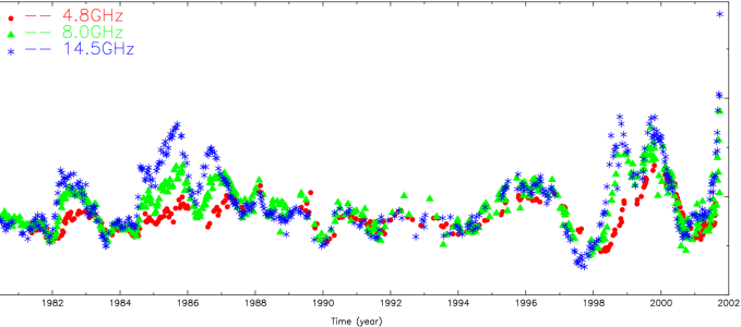
Figure 5: Light curves of 1156+295 at 4.8, 8.0 and 15 GHz from the monitoring data of the University of Michigan Radio Astronomy Observatory.

Table 4: The results of model fitting at kiloparsec scales

Observation inf.	$S_{total}$	Comp	$S_{c}$	r	$P.A.$	a	b/a	$P.A.$
	(mJy)		(mJy)	(mas)	($\degr$)	(mas)		($\degr$)
(1)	(2)	(3)	( 4)	(5)	(6)	(7)	(8)	(9)
1997.14	1668	D	1608	0.0	$0.0$	8.4	0.25	15.2
MERLIN		D6	21.5	53.7	$-8.5$	18.6	1.0	0
5 GHz		D4	11.4	515	$-19.3$	132	1.0	0
		D3	13.2	737	$-18.2$	76.9	1.0	0
		D2	7.4	1027	$-10.8$	101	1.0	0
		D1	13.9	1948	$-18.4$	135	1.0	0
Errors			8%	9%	3	9%		3
1999.14	2290	D	2214	0.0	$0.0$	8.6	0.38	15.6
MERLIN		D6	28.5	56.9	$-6.0$	23.9	1.0	0
5 GHz		D4	13.1	545	$-20.6$	130	1.0	0
		D3	14.0	743	$-18.0$	70.0	1.0	0
		D2	11.2	1057	$-12.0$	138	1.0	0
		D1	16.6	1938	$-18.3$	128	1.0	0
Errors			8%	9%	3	9%		3
2000.92	1666	D	1640	0.0	$0.0$	5.8	0.6	25.1
VLA		D3	7.5	747	$-16.1$	102	1	0
22.5 GHz		D1	4.6	1960	$-17.9$	88.0	1	0
Errors			7%	7%	3	7%		3
1997.41	1768	D	1540	0.0	$0.0$	10.1	0.7	15.0
MERLIN		D5	27.8	201	$-27.6$	46.9	1.0	0
1.6 GHz		D4	15.0	480	$-19.7$	70.1	1.0	0
		D3	42.1	716	$-18.4$	105	1.0	0
		D2	17.4	1109	$-12.8$	183	1.0	0
		D1	37.6	1945	$-18.7$	137	1.0	0
		DN	45.7	2055	$-2.0$	1409	0.5	59.5
		Db	20.6	138	$147.6$	156	1.0	0
		Da	11.1	1398	$144.9$	694	1.0	0
		DS	27.6	2152	$-161.5$	1217	0.6	$-75$
Errors			8%	9%	3	9%		3
2000.92	1042	D	1000	0.0	$0.0$	13.5	0.7	22.3
VLA		D5	2.2	198	$-26.5$	70.4	1.0	0
8.5 GHz		D4	3.2	507	$-22.9$	85.0	1.0	0
		D3	10.1	734	$-17.6$	135	1.0	0
		D2	3.8	1128	$-13.6$	231	1.0	0
		D1	9.2	1945	$-18.2$	135	1.0	0
		DN	6.6	2121	$-2.3$	1305	1.0	0
Errors			7%	7%	3	7%		3

Fig. 5 shows the light curves of 1156+295 at 4.8, 8.0, and 15 GHz measured at the University of Michigan Radio Astronomy Observatory (UMRAO). Several flares from 1980 to 2002 were detected.

The intensity of a flare is stronger at higher frequencies. Flares at different frequencies do not occur simultaneously: high frequency flares appear early. Similar results have been reported in some other sources (Bower et al. (1997), Wehrle et al. (1998), Zhou et al. (2000)). The lags are consistent with the fact the flares components are optically thick and short wavelengths peak first, which can be seen directly from the light curves (Fig. 5).

The strongest flare recorded over the last 20 years started at the beginning of 2001. The available data show a maximum in the flux density of 5.7 Jy at 14.5 GHz in September 2001. The next strongest flare began in October 1997 at 8.4 and 14.5 GHz, and reached its peak in October 1998 with a flux density of 3.6 Jy at 14,.5 GHz. Another similar peak occurred in September 1999. Such double peaked flares are also seen in the period from 1985 to 1987. The separations of the double peaks are about one year.

Figure 6: A helical pattern for 1156+295: vector S is the direction of the line of the sight, vector V is the direction of the velocity of the jet, $\theta(t)$ is the viewing angle between V and S.

Figure 7: The differential image of the two 5 GHz MERLIN data-sets from the epoch 1999.14 and 1997.14, Peak flux density is 0.6 Jy/beam. Contour levels are 0.5 mJy/beam $\times(-4,-2,-1,1,2,4,8,16,32,...$), FWHM: 80 $\times$ 80 mas.

A possible explanation for the ’double-peak’ is that only one jet component is ejected with a helical trajectory on the surface of a cone. The emission of the jet component is then enhanced along the path but only when it points toward the observer. If two nearby pitch angles (or multi pitch angles) are close to the line of the sight, we can observe double peaked flares (or multi peaked flares) with the maximum Doppler boosting from one ejected component. In the case of 1156+295, this results in two distinct peaks in the total flux density measurements. If the jet components always travel along a helical path aligned with the line-of-sight then double peaks should always appear in the light curves. In particular, double peaks should appear at the outburst near 2002. In this case, as shown in Fig. 6, we find one maximum for Doppler boosting at the each helical cycle. Then the peak separation time of double peaks $\Delta t_{pk}$ should be the period of the first detectable helical orbit and can be directly inferred as the period of the precession of the jet-base. The pure geometrical model described here is similar to the lighthouse model proposed by Camenzind & Krockenberger (CK92 (1992)). However, in the case of 1156+295, the observed period of the peak of its flux density is somewhat longer than that in the lighthouse model.

Two jet components ejected one after the other can also explain the ’double-peak’ pattern. If these two jet components move out from the radio core, they might be resolved from each other by high resolution VLBI images. Further multi-epoch VLBA observations at higher frequencies (2cm, 7 and 3 mm) are currently underway, which will help to clarify the issue.

The peak brightness detected in our multi-epoch VLBI observations varies in phase with the total flux density measurement made at UMRAO. This indicates the most outbursts take place in the core area and/or in the unresolved inner-jet.

4 Morphology and structural variability on kpc-scales

4.1 Model fitting the MERLIN and VLA data

The MERLIN and VLA visibility data were fitted with elliptical Gaussian components using DIFMAP. The results of model-fitting are presented in Table 4. Column 1 gives the observation epoch, array, and observed frequency. The total CLEANed flux density of the image is listed in column 2, followed by the component’s name in column 3. Column 4 shows the flux density of the component. This is followed in columns 5 and 6 by the radial distance and position angle of the component (relative to the core component). The next three entries (columns 7 to 9) are the major axis, axis ratio and position angle of the major axis of the fitted component. The uncertainties of the model fitting listed in Table 4 are estimated using the formulae given by Fomalont (Fomalont (1999)).

Besides the core component D, six components (D1 to D6) are fitted in the northern jet (see Fig. 1b). Two counter jet components (Da and Db) and two lobe components (DN and DS) are detected in the 1.6 GHz MERLIN data (as labelled in Fig. 2a). D5 is too faint to be well fitted in the 5 GHz MERLIN data (Fig. 1a&b). D6 is not fitted with the 1.6 GHz MERLIN and 8.5 GHz VLA data because of the limitation of the resolution (Fig. 2). Only three main components (D, D1 and D3) are detected in the 22.5 GHz VLA data (Fig. 1c).

From columns 2 and 4 of Table 4, it is clear that more than 95 $\%$ of the flux density came from the core at all frequencies, except 87$\%$ at 1.6 GHz. This is consistent with the flux density of the core being enhanced by beaming effects while the extended emission is not.

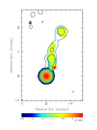
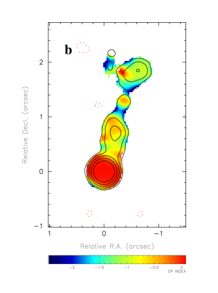
Figure 8: (a): A simultaneous spectral index distribution between 8.5 and 22.5 GHz at the epoch 2000.92 (color), superimposed on the 8.5 GHz VLA image; the wedge at the bottom shows the spectral index range $-2.5$ to 0.5; (b): A 1.6 - 5 GHz non-simultaneous spectral index distribution (color), superimposed on the 5 GHz MERLIN image at the epoch 1997.14; the wedge at the bottom shows the spectral index range $-2.4$ to 0.08. The contours levels in both b&c are 0.5 mJy/beam $\times$ ($-1,1,4,16,64,256$) with FWHM of 200$\times$200 mas.

Figure 9: Slice plots of spectral index at p.a. -18°, corresponding to Fig. 8a and Fig. 8b respectively.

The two main kpc-scale components (D1 and D3) are almost at the same position angle, $\sim-18\degr$, in all MERLIN and VLA images, and their FWHMs are comparable at 1.6, 8.5, and 22 GHz, while D3 is more compact than D1 at 5 GHz. We note that D2 and D4 sometimes appear to have larger FWHMs than that of D1 and D3, which may be attributed to using circular Gaussian components for model fitting.

A counter jet component (Db) is fitted in the 1.6 GHz MERLIN data (see Fig. 2a). It is located at about 138 mas from the core at $p.a.\sim 147\degr$. Two other low brightness components are also detected (labelled as Da and DS in Table 4 and Fig. 2a).

The lobe to counter-lobe (the components DN and NS) flux density ratio at a distance of 2 arcseconds from the core is $J_{lobe}=1.66$. The distance and size of the counter-jet component Da allow us to assume that its corresponding structural pattern in the jet should include the components D2 and D3. Under this assumption, the flux density ratio (D2+D3) to counter-jet Da is $J_{kpc-jet}=5.36$. No clear jet component corresponding to Db is evident in Fig.2a. This might be due to the corresponding jet component being embedded in the core.

4.2 Structural variability on kpc-scales

The two 5 GHz MERLIN observations with a time separation of two years (the epochs 1997.14 and 1999.14) allow us to study structural variability. As we mentioned in section 3.3, the source was in its lowest state around 1998, immediately before a strong flare occurred (see Fig. 5). The model fitting results show that the flux density of the core component D increased by 37% from 1997 to 1999 (Table 4), which is most easily explained in terms of an outburst occurring in the inner core.

To study the variation in the jet radio structure directly from the images, we subtracted the image in Fig. 1a from that in Fig. 1b ($F1b-F1a$) to obtain a differential image (Fig. 7). In order to minimize the adverse effects of a limited dynamic range in the presence of the bright core, we first subtracted the core component of 1.5 Jy from the two MERLIN data-sets (epochs 1997.14 and 1999.14), re-imaged the residual uv-datasets, and then produced the differential image presented in Fig. 7.

The largest difference in the flux densities comes from the core. The peak brightness of the differential image is 0.6 Jy/Beam. Some variations at a level of 1 mJy per beam in the jet were found.

The increased flux density in the core can be explained as a flare in the compact unresolved component, as we can see in the light curve in Fig. 5. Both positive and negative variations are found above the uncertain set by the noise in the original images (see Fig. 1a&b) in the first 0.5$\arcsec$ of the jet (see Fig. 7). This may be attributed to the continuous movement of the jet. The variations in the areas of D1 and D3 can not be affected by the flare from the core, since it would take a few thousand years to propagate through the distance of 2$\arcsec$ at the speed of light. This leads to the conclusion that some flares may occur, independently from the core, in the knot (D3) and hotspot (D1).

4.3 Spectral index distributions on kpc-scales

Multi-frequency observations with the VLA and MERLIN allow us to produce a spectral index distribution of the source on the kpc scale (S${}_{\nu}\propto\nu^{\alpha}$). A spectral index distribution obtained with simultaneous VLA data at 8.5 and 22.5 GHz is presented in Fig. 8a by aligning the peak emission of the cores. An upper limit to the opacity shift of 13 mas was estimated for the optically thin component D3, while a frequency-dependent position difference of the core of 7 mas was estimated with Lobanov’s model (Lobanov (1998)).

We also present a non-simultaneous spectral index distributions based on the MERLIN data between 1.6 GHz (epoch 1997.41) and 5 GHz (epoch 1997.14) in Fig. 8b without consideration of the opacity shift. An upper limit to the opacity shift of 20 mas was estimated by comparing the modelfit results of jet component D3, and 7.4 mas of frequency-dependent position difference of the core was estimated (Lobanov (1998)).

The spectral index distributions of the source (Fig. 8a&b) show that the strongest compact component has a flat spectrum.

A steep spectrum ring appears around the core in Fig. 8a since the size of the core at 22 GHz is only about half of that at 8.5 GHz.

The kpc scale jets clearly have a steeper spectrum than the core (see Fig. 8a$\&$b). There is also a general steepening of the radio emission towards the edges of the jet emission. Some isolated flat spectrum spots in the jet are also observed, especially in Fig. 8b. These may be real or due to the observations being made at different epochs.

Slice plots of the spectral index distributions along the jet axis at position angle of -18° are shown in Fig. 9, corresponding Fig. 8a and 8b, respectively. The slice lines do not intersect the peak of the each component since the components are not aligned on a straight line. We can also estimate the spectral indexes with the modelfit results of Table 3 (see Table  5).

It is clear that the core has a flat spectral index, while the jet components D1, D2, , D3 and D4 have steep spectral indexes. Each component has a steep spectrum edge.

Table 5: The spectral index on the kpc scale

Bands D D1 D2 D3 D4

8.5 - 22.5 GHz 0.51 $$-0.7$$

1.6 -  5.0 GHz 0.04

5 Morphology and structural variability on pc-scales

5.1 Model fitting of the VLBI data

Table 6: Model-fitting of the VLBI data

Obs. inf. Comp $$S_{c}$$ r a b/a

(mJy) (mas) () (mas) () () K K

(1) (2) (3) (4) (5) (6) (7) (8) (9) (10) (11) (12) (13) (14)

1996.43 C 2097 0.0 0.55 0.24 15.8 15.5 2.5 1.6

VLBA C3 141.2 3.22 1.48 1.0 11.4 3.4 5.3

C Band C2 133.9 4.92 1.88 1.0 13.8 3.6 3.1

C1 129.5 11.01 9.05 0.67 2.0

Errors 12% 15% 7 16% 7

1997.14 C 1109 0.0 0.51 0.41 5.0 6.0 0.9 1.8

EVN C3 117.8 3.95 1.69 1.0 13.6 8.9 3.5

C Band C2 172.4 5.06 3.93 1.0 21.2 7.5 9.4

Errors 18% 20% 10 20% 7

1997.42 C 927.3 0.0 0.90 1.0 5.3 4.3 0.9 1.7

VSOP C3 135.0 3.01 2.05 1.0 13.1 8.8 2.7

L Band C2 240.2 5.66 4.11 1.0 20.3 7.3 1.2

C1 104.4 10.97 5.73 1.0 2.7

Errors 17% 15% 10 20% 7

1998.12 C 504.0 0.0 1.0 0.39 0.5 0.9 1.1 …

Global C3 89.9 3.71 1.75 1.0 2.5

C Band C2 95.4 5.59 2.66 1.0 1.1

C1 82.6 10.10 7.84 1.0 1.1

Errors 18% 10% 10 10% 7

1999.01 C 2245 0.0 0.15 0.37 17.1 22.4 2.5 1.4

VLBA C4 26.3 1.25 0.8 1.0 12.7 3.3 3.8

U Band C3 17.7 4.19 1.5 1.0 11.8 3.0 7.4

C2 28.0 6.23 2.6 1.0 14.0 3.1 3.8

Errors 15% 13% 5 13% 7

1999.14 C 1387 0.0 0.39 0.40 12.3 11.8 2.0 1.6

EVN C4 42.2 1.55 1.1 1.0 11.9 4.6 2.9

C Band C3 31.9 4.26 1.2 1.0 10.6 4.6 1.8

C2 76.3 5.83 2.3 1.0 13.7 4.6 1.2

C1 71.7 10.62 6.6 1.0 1.3

Errors 15% 15% 6 15% 7

1999.45 C 1765 0.0 0.35 0.44 18.5 12.4 2.7 1.4

Global C4 52.9 1.55 1.33 1.0 13.1 2.8 2.4

C Band C3 54.1 4.31 2.06 1.0 12.3 2.7 1.1

C2 108.5 6.14 3.55 1.0 14.3 3.0 7.4

C1 92.1 11.2 8.07 1.0 1.2

Errors 9% 10% 5 10% 5

2000.12 C 931.3 0.0 1.6 0.28 6.1 4.8 1.1 1.8

VLBA C2&3 245.1 5.23 3.9 1.0 15.1 7.5 1.3

L Band C1 195.0 10.53 7.9 1.0 2.5

C0 88.1 31.66 25.4 1.0

Errors 10% 12% 5 13% 5

The VLBI self-calibrated data-sets associated with each image in Fig. 3 were fitted with Gaussian components using DIFMAP. An elliptical Gaussian component was fitted to the strongest component, and circular Gaussian brightness distributions were used for the jet components to estimate their sizes.

The parameters of model fitting are listed in Table 6. Column 1 gives the observation epoch, array, and frequency. columns 2 to 8 are the same as the columns 3 to 9 in Table 4. The uncertainties of the model fitting are estimated in the same way as for the acrsecond-scale images (see section 4.1) and are listed in the table.

Five components are fitted to the VLBI data. In order to compare our results with previous publications, we label the components following the convention introduced by Piner and Kingham (1997) from C to C4 (see Fig. 10).

Fig. 10 is the model-fitted image (Gaussian components restored with a $2.4\times 1.1$ mas, at $p.a.-2.1\degr$ beam) of 1156+295 based on the Global VLBI data at the epoch 1999.45 at 5 GHz. This is in good agreement with the CLEANed image shown in Fig. 3g.

The core contributes a higher fraction of the total flux density at higher frequencies. The fraction of the core flux density is about 97$\%$ at 15 GHz, 80 - 86$\%$ at 5 GHz (except the lowest level of 65$\%$ at the minimum of activity at the epoch 1998.12), and 65 - 70$\%$ at 1.6 GHz. This is a clear indication that the high frequency emission comes from the inner regions of the source. The fraction of the core flux density is higher during active outburst phases (e.g. 85$\%$ at the epoch 1999.45 at 5 GHz) compared to more quiescent epochs (e.g. 65$\%$ at the epoch 1998.12 at 5  GHz). This suggests that most of the flare occurred in an area less than 1 mas in size.

For the individual components, we note: a) we use one elliptic Gaussian component C1 to fit the two separated outer emission regions in the north-east area at epoch 1996.43 (Fig. 3a); b) C1 is not detected at the epoch 1997.14 due to sensitivity limitations and is resolved at 15 GHz (epoch 1999.01); c) components C2 and C3 are not resolved in the 1.6 GHz VLBA observations and are fitted as a combined centroid component C2&3; d) C4 is detected after 1999 at 15 GHz; e) outer component C0 is detected at a distance of 30 mas from the core (Fig. 3h).

Figure 10: The model image at the epoch 1999.45 at 5 GHz. Peak brightness is 1.71 Jy/beam. Contour levels are 1.5 mJy/beam $\times(-1,1,1,4,16,64,256)$.

5.2 The differential VLBI image at 5 GHz

As noted in section 5.1, the largest structural variations during the flare appeared in the vicinity of the core. The two high sensitivity global VLBI observations at 5 GHz (epochs 1998.12 and 1999.45) were made in the states of low and high flaring activity respectively. The differential image of these two global VLBI datasets ($F3g-F3d$) is shown in Fig. 11. Most of the different flux density in the image comes from the core area. The peak (residual) flux density is 1.3 Jy/beam, which is about 3 times of that of the total intensity peak observed at the epoch 1998.12. This large difference in the core region is clearly associated with the violent flare in the core that has occurred after the epoch 1998.12 and during the epoch 1999.45.

The existence of a ‘negative emission’ component in the differential image (Fig. 11) can be explained by a variation in the direction of the jet. When the direction of the relativistic jet comes close to the line of sight, its flux density is enhanced by a Doppler boosting; when the orientation of jet changes from the line of sight, the component becomes fainter. This pattern is characteristic of a relativistic jet with a helical trajectory.

The observed feature can be also explained directly by the proper motion of the jet. If one component moves from point A to point B, an observer will see a negative component at the point A and a positive component at point B with the same absolute value of flux density. This seems not like in the case of Fig. 11.

Figure 11: The differential image of the two 5 GHz Global VLBI data-sets from the epochs 1999.45 and 1998.12, the peak brightness is 1.3 Jy/beam., contour levels are 2.0 mJy/beam $\times(-8,-4,-2,-1,1,2,4,8,16,32,...,512)$. FWHM: 2 $\times$ 1 mas, at $0\degr$

5.3 Proper motion of the jet components

Figure 12: Apparent proper motion of the jet components: 1.6 GHz (diamond), 5 GHz (star), 15 GHz (square), 22 GHz (triangle, Jorstad, et al. 2001).

The positions of the components during the period from 1996 to 2000 are shown in Fig. 12. The x-axis is the time and the y-axis shows the distance of the components from the core. Different symbols are used to represent different observing frequencies: a diamond for 1.6 GHz, a star for 5 GHz, and a square for 15 GHz. We also plot a triangle for the 22 GHz component labelled as B2 by Jorstad et al. (2001). We identify B2 is the same with the component C4 in this paper (see Table 4, Fig. 10). The components C2 and C3 are not resolved at 1.6 GHz at the epoch 2000.12. This combined centroid is shown as a filled diamond symbol.

Since the positions of the components could be frequency dependent, we estimate the proper motion of components C2, C3 and C4 via the 5 GHz data sets. These are 0.39$\pm$0.1, $0.30\pm 0.08$ and $0.34\pm 0.08$ mas/yr respectively. These values correspond to the apparent velocities of $13.7\pm 3.5,10.6\pm 2.8$, and $11.8\pm 2.8c$.

The component C1 is located at the point where the jet turns sharply. It does not appear to have any appreciable motion in the r direction, while the position angle changed from about 35°to 31°, which correspond to a apparent velocity of about 7$c$.

Jorstad et al. (2001) reported the proper motion measured at 22 GHz of three components in this source, the period of the VLBA observation is overlapped with ours, the reported apparent velocity of B2 (labelled as C4 in this paper) is $11.8\pm 1.2$ (corrected to $q_{0}=0.5$), based on three epochs during period 1996.60 to 1997.58, which is in agreement with our result. The B3 component in their paper is unresolved in our VLBI data due to the limited resolution at low frequencies. Piner & Kingham (1997) reported that the apparent velocities of C1 to C4 are $13.5\pm 3.5,8.1\pm 1.7,8.5\pm 1.4$, and $5.4\pm 1.8\leavevmode\nobreak\ c$, respectively, based on their geodetic data obtained during the period 1988.98 to 1996.25.

The apparent radio component velocity of 40$c$ is the highest super-luminal velocity reported for AGN to date (McHardy et al. (1990); McHardy et al. (1993)). However, as this value was derived based on four-epoch of VLBI observations at three frequencies, the apparent motion could be ’caused’ by frequency-dependent effects.

5.4 Spectral index distribution on pc-scales

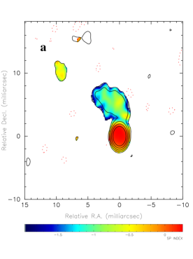
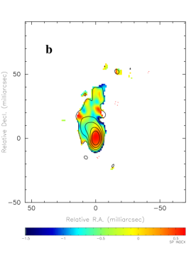
Figure 13: (a): The 5 $vs$ 15 GHz spectral index distribution (color), superimposed on the 15 GHz VLBA image at the epoch 1999.01, the wedge at the bottom shows the spectral index range $-1.95$ to 0.25; (b): the 1.6 $vs$ 5 GHz spectral index distribution (color), superimposed on the 5 GHz VLBA image, the wedge on the bottom shows the spectral index range $-1.5$ to 0.62. The contours levels in a & b are 2 mJy/beam $\times(-1,1,4,16,64,256)$ with FWHM of 1.5$\times$1 mas and 7$\times$4 mas, respectively.

Although no simultaneous VLBI data of the source at different frequencies are yet available, we attempted to estimate the spectral index distribution of the jet on pc scales using the multi-epoch/multi-frequency images presented here. The non-simultaneous spectral index distribution between 1.6 (epoch 2000.15) and 5 GHz (epoch 1999.45), as well as between 5 (epoch 1999.45) and 15 GHz (1999.01) are presented in Fig. 13 by summing the zero opacity shift in the cores. The upper limit opacity shift of 0.3 and 0.7 mas were estimated by comparing the modelfit results of the optical thin jet component for Figs. 13a and 13b, respectively. Meanwhile, 0.5 mas of the uncertainty of the frequency-dependent position difference of the core was estimated with Lobanov’s model (Lobanov (1998)) for the spectral index maps Figs. 13a and 13b.

Fig. 13a shows the 5$-$15 GHz spectral index distribution. It is clear that the core area has a flat spectrum $\alpha\sim 0.25$. The emission becomes a steep spectrum ($\alpha\sim-0.7$ to $-1.5$) outwards from the core.

Fig. 13b is the 1.6$-$5 GHz spectral index distribution. There is an inverse spectrum ($\alpha\sim 0.58$) in the core area. Two flat spectrum features are seen in the jet.

Figs. 14a and 14b show the profile of the 5$-$15 GHz spectral index along the direction of P.A.=0° and $1.6-5$ GHz spectral index along P.A.= 25°, corresponding to Figs. 13a and 13b, respectively.

Table 7 gives the spectral index values estimated from the model-fit components listed in Table 7.

Table 7: The spectral index on the pc scale

Bands C C1 C2 C3 C4

5 - 15 GHz 0.22 $$-1.2$$

1.6 - 5 GHz 0.58

Figure 14: (a): Slice plot of the spectral index at p.a. 0° corresponding to Fig. 13a; (b): Slice plot of the spectral index at p.a. 25° corresponding to Fig.13b

6 Physical parameters of the core and jet

6.1 The Equipartition Doppler factor $\delta_{eq}$

As we mentioned in the previous sections, the flares of 1156+295 may be enhanced by the Doppler boosting. The Doppler factor of the outflow from compact radio cores can be estimated assuming the energy equipartition between the radiating particles and the magnetic field (Readhead (1994); Guijosa & Daly (1996)).

The method was considered using the radio observed parameters at the turnover frequency, but actual VLBI observations were not done at the turnover frequency. We will use the radio parameters we obtained from our VLBI observations to roughly estimate the Doppler boosting in 1156+295.

By following the assumptions of Scott $\&$ Readhead (1977) and Marscher (1987), the Equipartition Doppler factor $\delta_{eq}$ of the core component for each epoch is estimated and listed in column 9 of Table 6. The values are in the range of 5 to 18.5 except 0.5 at the epoch 1998.12. The latter is expected, since the source is at its lowest state.

6.2 Inverse Compton Doppler factors $\delta_{IC}$

For comparison, the Doppler factor of the core component can also be estimated with the Synchrotron self-Compton emission in a uniform spherical model (Marscher (1987)).

Under the assumption in section 6.1, we estimated $\delta_{IC}$ using the equation (1) of Ghisellini et al. (1993) with the $0.075\leavevmode\nobreak\ \mu$Jy X-ray flux density of 1156+295 at 2 keV (McHardy (1985)). The inverse Compton Doppler factors $\delta_{IC}$ of 1156+295 at all epochs were listed in the column 10 of Table 4. The values cover a wider range from 4.3 to 22.4 except 0.9 at the epoch 1998.12.

The estimated values may be a lower limit since part of X-ray emission could come from the thermal or other emission. The variability of X-ray flux and non-simultaneous observations between radio and X-ray are causes of uncertainty in estimating $\delta_{IC}$.

The $\delta_{IC}$ and the $\delta_{eq}$ are comparable. The average values of $\delta_{IC}$ is about 96% of that of $\delta_{eq}$. The Doppler factor varied with time. The variation was correlated with the total flux density variation of the source. The core has higher Doppler factor at a higher frequency than that at lower frequencies.

6.3 Lorentz factor and viewing angle

In the relativistic beaming model $\beta_{app}$ depends on the true $\beta(v/c)$ factor and the angle to the line of sight $\theta$ (Rees & Simon, (1968)),

$$\beta_{app}=\frac{\beta\sin\theta}{1-\beta\cos\theta}\;\;.$$ (1)

The Doppler factor can be written as

$$\delta=\gamma^{-1}(1-\beta\cos\theta)^{-1}\;\;,$$ (2)

where $\gamma=1/\sqrt{1-\beta^{2}}$.

The Lorentz factor $\gamma$ and the viewing angle $\varphi$ can be computed (Ghisellini et al. 1993):

$$\gamma=\frac{\beta_{app}^{2}+\delta^{2}+1}{2\delta}\;\;,$$ (3)

$$\tan\varphi=\frac{2\beta_{app}}{\beta_{obs}^{2}+\delta^{2}-1}\;\;.$$ (4)

The $\gamma$ and $\phi$ of C2, C3, and C4 shown in columns 11 and 12 of Table 4 are estimated from the Doppler factor ($\delta=\delta_{eq}$ is used) and their apparent velocities $\beta_{app}$. The Lorentz factor of each epoch changes between 13.8 and 21.2, 10.6 and 13.6, 11.9 and 13.1 for C2, C3 and C4, respectively, while the viewing angles varied in the range of 2.7$\degr$ to 8.9$\degr$.

Ghisellini et al. reported that the jet to counter-jet brightness ratio can be estimated from (1993):

$$J=(\frac{1+\beta\cos\theta}{1-\beta\cos\theta})^{2-\alpha}\;\;.$$ (5)

Taking $J_{kpc-jet}=5.36$ and $J_{lobe}=1.66.$ (see section 4.1), and assuming the spectral index of the kpc jet and the lobe $\alpha=-0.9$ (Table 5), we have:

$$(\beta\cos\theta)_{kpc-jet}=0.3\;\;,$$ (6)

$$(\beta\cos\theta)_{lobe}=0.1\;\;.$$ (7)

It indicates that the kpc jet is faster and/or has a smaller viewing angle than the lobe components.

6.4 The brightness temperature

A high brightness temperature in flat spectrum radio sources is usually considered to be an argument supporting relativistic beaming effect. In the synchrotron model, with the brightness temperature close to $\sim 10^{12}$ K, the radiation energy density dominates the magnetic energy density, and produces a large amount of energy in a very short time scale. The relativistic particles quickly cool (Compton catastrophe). The maximum brightness temperature that can be maintained is about $\sim 10^{12}$ K in the rest frame of the emitting plasma (Kellermann & Pauliny-Toth (1969)).

Figure 15: The brightness temperature distribution of VLBI components: 1.6 GHz diamond, 5 GHz circle, 15 GHz triangle.

The brightness temperature $T_{b}$ of an elliptical Gaussian component in the rest frame of the source is (Shen et al. (1997))

$$T_{b}=1.22\times 10^{12}\frac{S_{\nu}}{\nu^{2}_{ob}ab}(1+z)\leavevmode\nobreak\ $K$\;\;,$$ (8)

where $z$ is the redshift, $S_{\nu}$ is the observed peak flux density in Jy at the observed frequency $\nu_{ob}$ in GHz, $a$ and $b$ are the major and minor axes in mas.

The brightness temperatures of the the components of 1156+295 are calculated with equation (8) at various epochs. The results are listed in column 13 of Table 4. We present the brightness temperature distribution in Fig. 15. It is clear that the component brightness temperatures are inversely proportional to their observed frequencies. The brightness temperature of the core component is around $10^{12}$ K, while the brightness temperatures of the jet components are much lower (around $10^{7-10}$ K).

By considering the Doppler boosting of the source, the intrinsic brightness temperature $T_{r}$ can be estimated as $T_{r}=T_{b}/\delta$ and listed in column 14 of Table 4 ($\delta_{eq}$ is used). The intrinsic brightness temperatures of the core component at all epochs are almost constant ($\sim\leavevmode\nobreak\ 10^{11}$K). This may serve as an upper limit of the brightness temperature in 1156+295 in the rest-frame of the source. Since the estimated $\delta_{eq}$ is an upper limit, the intrinsic brightness temperatures here are the lower limit.

7 A helical pattern

The helical jet model for AGNs was proposed (e.g. Conway & Murphy, (1993)) to explain a bi-modal distribution of the difference in the orientation of arcsecond and mas structures in core-dominated radio sources. Helical jets are a natural result of precession of the base of the jet (e.g. Linfield 1981) or fluid-dynamical instabilities in the interface between the jet material and the surrounding medium (Hardee 1987). Assuming the initial angular momentum of the jet is due to the precession of the accretion disk, the helical structure observed might be related to the precession of a wobbling disk while the interface instability produces a wiggling structure that reflects a wave pattern (e.g. Zhao et al. (1992)).

As we mentioned in section 3.3, the trajectory of the jet in 1156+295 could be a helix on the surface of a cone (Fig. 6). Fig. 16 shows the measured position angles of all components at all frequencies and all epochs for 1156+295. The two components (B2 and D) from the Jorstad et al’s paper (2001) are also included. The x-axis shows the distance of the components from the core in logarithmic scale and the y-axis shows the position angle. This symmetric distribution of the position angle suggests that the jet in 1156+295 is spatially curved and the jet components follow a helical path.

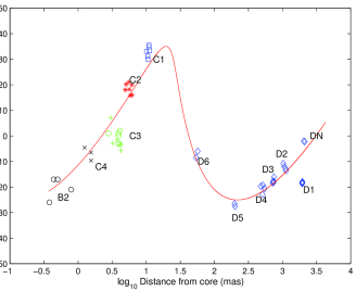
Figure 16: Measured positions of all components at all frequencies and all epochs for 1156+295.

By assuming the conservation laws for kinetic energy and momentum, the helical model parameters can be derived following (Steffen et al (1995)):

$$z(t)=\beta_{z}t+z_{0}\;\;,$$ (9)

$$r(t)=\beta_{z}t\;\;{\rm tan}\psi+r_{0}\;\;,$$ (10)

$$\phi(t)=\phi_{0}+\frac{\omega_{0}r_{0}}{\beta_{z}\;\;{\rm tan}\psi}\;\;{\rm ln}\frac{r(t)}{r_{0}}\;\;,$$ (11)

where $z,r,\phi$ are the cylindrical coordinates; $\beta$ is the velocity of the jet component in units of the speed of light; $\psi$ is opening half-angle of the cone; $t$ is the time in the rest frame of the source (jet); and $\omega$ is the angular rotation velocity ($d\phi/dt$).

The estimated viewing angles $\theta$ of inner jet components in 1156+295 are 3$\degr$ to 8$\degr$ (see table 4). A value of $5\degr$ was adopted as the angle between the line of sight and the axis of the cone; the half-opening angle of the cone $\psi$= 2.5$\degr$ was estimated from the observed oscillatory amplitude of position angle. Figs. 16 and 17 show one possible approximation rather than the best fit to the data. Fig. 16 represents the relationship between the position angle and the projected distance from the core of this helical jet. Fig. 17 shows the projected path of this helical trajectory in the image plane on the two different scales. These figures show that a simple helical trajectory can well represent the radio structure from 1 mas to 1 arcsecond (D2 component).

Beyond the D2 component, the helical path is probably interrupted or it changes direction due to the interaction between the jet and the medium. The model does not consider scales less than 1 mas because of the lack of observational data. Jorstad et al. (2001) pointed out that the trajectories of components can fall anywhere in the region of position angle from $-25\degr$ to 25$\degr$ out to a distance of $\sim$ 1 mas from the core based on their data at 22 GHz. This does not contradict the helical model presented here.

Fig. 18 shows that the components move along curved path. For comparison, we also included the data from the geodetic VLBI observation by Piner & Kingham (1998) (estimates from their Fig. 10) during period from 1988 to 1996 in Fig. 18, labelled as PKC1, PKC2 and PKC3. The two data sets show the movement of jet components along a curved trajectory on the time scale of 20 years.

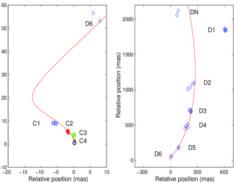
Figure 17: The positions of jet components and the projective path of a helical jet in the image plane on the pc-(left) and the kpc-(right) scales.

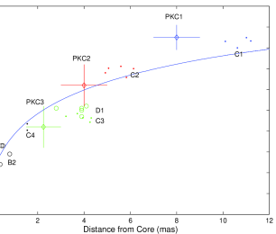
Figure 18: The evidence for the movement of the components along a curved path.

In addition, we note some small structural oscillations observed on the mas scale (e.g. components C3 and C1). It is not clear whether this is a processing on a short time scale or measurement errors.

If the jet moves on the surface of a cone along a helical trajectory, the helical wavelength ($\lambda$, the pitch distance) of this helical trajectory increases with the time. The apparent period of this helical jet (starting at about 1 mas from the core) at the projected distance is about 1200 mas. If we assume that the averaged proper motion ($\mu$ = 0.3 mas/yr) is constant on the 1 mas to 1 arcsecond scale (as we assumed), the lower limit of the helical period in time in the source-rest frame is about $10^{4}$ years ($P=(1+z)*\lambda$/$\mu$). Considering the possible deceleration of the jet on the large scale, the real period is likely to be longer.

The helical jet may be due to a binary black hole in the nucleus of the source, such as in the BL Lac Object OJ 287 (e.g. Sillanpaa et al. (1988), Lehto & Valtonen (1996)). The model for both the optical and radio light curves observed in OJ 287 suggests that the helical jet and double peaked cyclic outbursts can be produced by a pair of super-massive black holes in a binary system (Villata et al. (1998)) if the twin jets ejected from each of the BHs were in a precession around the orbital axis of the binary and the Doppler boosting effect is important.

Alternatively, in a spinning super-massive black hole system, if the disk axis offsets from the spin axis, the intrinsic torque of the spin black hole placing on an accretion disk could also produce a precession of the axis of the accretion disk (Liu & Melia (2002)). The variation of the direction in the jet motion produced from a wobbling disk can also be responsible for the helical pattern.

8 Summary

We investigated the radio structures of the radio-loud quasar 1156+295 in detail on various angular scales using different interferometric arrays at different frequencies.

1. The source shows an asymmetric double structure at l.6 GHz with 250 mas resolution (about 1.5 kpc), the northern jet is relativistically Doppler boosted, the southern emission is resolved into several low brightness regions (see the color figure of the cover).

2. At 80 mas resolution (about 0.5 kpc), the northern jet has an almost straight structure at $P.A.=-18\degr$ with some sinusoidal fluctuations. The source is dominated by a flat core, and the jet emission has a steep spectrum.

3. On the VLBI scale, the jet bends from the north to the north-east at 3$\sim$4 mas from the core, and then turns about $90\degr$ to the north-west, thus aligning with the direction of the arcsecond-scale jet. The 1.6 GHz VLBA image links the VLBI emission and arcsecond emission of the jet, which follows an S type structure. This may be an evidence of a helical jet. The spectral index distribution at the mas scale shows a flat spectrum VLBI core and a steep spectrum jet. The differential image demonstrates that the flux density variation mainly comes from the very compact core area.

4. The proper motions in three components were detected; the apparent superluminal velocities are in the range of $10.6$ to $13.7\leavevmode\nobreak\ c$. The differential images also show evidence of bulk motion of the emitting material along a curved trajectory.

5. Ejection of the VLBI components corresponds to the flares in the light curves. This is consistent with the hypothesis that total flux density variations mainly occur in the core region.

6. High Doppler factors ($\sim$18), and a high Lorentz factor ($\sim$21) were measured in the northern jet components on pc-scales supporting the assumption that the jet moves relativistically.

7. We found that a helical trajectory along the surface of a cone can well represent the radio structure from 1 mas to 1000 mas, based on the conservation laws for kinetic energy and momentum. The period of the helical path is longer than $10^{4}$ years.

The study provides the most comprehensive account so far of kpc- and pc-scale morphological properties of the radio emission in the AGN 1156+295. These properties are analyzed in the framework of the jet helical model e.g. a binary black hole in the nucleus of the source. However, other models, e.g. based on the Kelvin-Helmholz instabilities (Hardee (1987)), the trailing shock model in a relativistic jet (Gomez et al. (2001)) or MHD processes could be verified in future studies against the observing data presented.