MAGIC: Exact Bayesian Covariance Estimation and Signal Reconstruction for Gaussian Random Fields

Abstract

In this talk I describe MAGIC MAGIC , an efficient approach to covariance estimation and signal reconstruction for Gaussian random fields (MAGIC Allows Global Inference of Covariance). It solves a long-standing problem in the field of cosmic microwave background (CMB) data analysis but is in fact a general technique that can be applied to noisy, contaminated and incomplete or censored measurements of either spatial or temporal Gaussian random fields. In this talk I will phrase the method in a way that emphasizes its general structure and applicability but I comment on applications in the CMB context. The method allows the exploration of the full non-Gaussian joint posterior density of the signal and parameters in the covariance matrix (such as the power spectrum) given the data. It generalizes the familiar Wiener filter in that it automatically discovers signal correlations in the data as long as a noise model is specified and priors encode what is known about potential contaminants. The key methodological difference is that instead of attempting to evaluate the likelihood (or posterior density) or its derivatives, this method generates an asymptotically exact Monte Carlo sample from it. I present example applications to power spectrum estimation and signal reconstruction from measurements of the CMB. For these applications the method achieves speed-ups of many orders of magnitude compared to likelihood maximization techniques, while offering greater flexibility in modeling and a full characterization of the uncertainty in the estimates.

I Introduction

Signal reconstruction from noisy data is one of the raisons d’être of applied statistics. If the signal is a Gaussian random field, and the signal and noise covariances are known in advance, Wiener filtering wiener ; rybickipress is the theoretically optimal method for estimating the signal from noisy data. In this simple case the solution is a linear operator that acts on the data vector and returns the minimum variance, maximum likelihood and maximum a posteriori estimator of the signal given the data.

What ought to be done, however, if the signal covariance is not known in advance, and the signal covariance must be estimated from the data? In fact there are applications where covariance estimation is the primary goal and signal reconstruction is secondary. These cases have traditionally been treated separately. For stationary signals, the covariance of the signal is best specified in the Fourier basis since this basis diagonalizes the covariance matrix. In these cases covariance estimation becomes power spectrum estimation. One such example is cosmic microwave background data (CMB) analysis which motivated this analysis. I will return to it in section IV. Other examples are time series analysis, spatial analysis of censored data, such as geological surveys, power spectrum estimation and signal reconstruction for helioseismology, image reconstruction based on a stochastic model of the form of pixel-pixel correlations, etc. The method described here generalizes the results of rybickipress and should therefore also be useful for the applications discussed there.

In this talk I will first review the common structure that underlies these apparently different statistical problems (section II). I will then summarize the main advances realized by the new method in section III. The subsequent section contains the results from the application of this new approach to the first all-sky CMB data set. Further details and examples can be found in our paper MAGIC and online materials at the conference WWW site.

The ideas in this paper were developed from a Bayesian perspective. There are pros and cons of Bayesian estimation. The pros are many: it maximizes the use of all available information and treats measurements, constraints and model on the same footing as information. The result of a Bayesian estimation is a probability density, not just a number, so one automatically obtains uncertainty information about the estimate. However, if Bayesian methods are implemented naively, these advantages come at the price of heavy computation especially for multivariate problems. However the results presented in this paper are an example that it is possible to overcome these computational challenges and make Bayesian techniques work in a highly multivariate ($D\sim 10^{6}$) problem.

II Signal Reconstruction and Covariance Estimation

In this section I will review the problems of signal reconstruction and covariance estimation from a Bayesian perspective. First, some notation. Let us assume that the data were taken according to the model equation

$$d=A(s+f)+n$$ (1)

where the $n_{d}$-vector $d$ contains the data samples, the ($n_{d}\times n_{s}$) matrix $A$ is the observation matrix, the $n_{s}$-vector $s$ is the (discretized) signal, the $n_{s}$-vector $f$ represents any contaminants (“foregrounds”) one has to contend with, and the $n_{d}$-vector $n$ is the instrumental noise. I model the signal stochastically (vs. a deterministic functional form) and “infer” its covariance properties from the data. In particular, the signal is modeled through its covariance properties, encoded in $S\equiv\langle ss^{T}\rangle$, the signal covariance matrix.

Then I can write the Bayesian posterior as

$$P(s,f,S|d,N)\propto P(d|s,f,N)P(s|S)P(f)P(S)$$ (2)

where $N$ is the noise covariance matrix $\langle nn^{T}\rangle$. I will now discuss the various terms in Eq. 2. The likelihood $P(d|s,f,N)$ specifies how the data is related to the quantities in the model. Given the model equation Eq. 1 specifies that $P(d|s,f,N)=G(d-A(s+f),N)$.

The other terms in Eq. 2 specify information about the components of the model. The term $P(s|S)$ contains information about the covariance of $s$. If $s$ is a Gaussian random field with zero mean (examples from cosmology are the CMB or other probes of the density fluctuations of matter on cosmological scales) $P(s|S)=G(s,S)$. Note that it is not assumed that $S$ is known.

Partial knowledge (or ignorance) about $S$ is quantified in terms of the prior $P(S)$. For a stationary field $P(S)$ might simply represent the fact that I parameterize the covariance matrix in terms of power spectrum coefficients. Eq. 2 also assumes that the signal, noise and the contaminants are stochastically independent of each other. Further, the equations as written are conditioned on perfect knowledge of the noise covariance.

Lastly, $P(f)$ encodes the knowledge or ignorance about foregrounds. Note that from a Bayesian perspective all that is required is that $P(f)$ accurately represents knowledge about $f$. Therefore assuming a Gaussian form for $f$ does not assume that $f$ actually has Gaussian statistics. In particular the mode of the Gaussian corresponds to the most probable (a priori) foreground model and the covariance to the uncertainty in the model. The ability to specify uncertainties in the foregrounds (which will then be taken into account when the method is applied) is a key feature of this approach which guards against biases from including incorrect foreground templates without the ability to account for the uncertainty in these templates.

Having specified the forms of the various terms on the right hand side of Eq. 2, the task is to explore the joint posterior density $P(s,f,S|d,N)$. However, traditionally the problem is treated in three different limits. If, as an expression of prior ignorance, I take $P(f)=const.$ and $P(s)=\int P(s|S)P(S)dS=const.$ then all the information is in the likelihood $P(d|s,f,N)$. In this case the best one can do if $n$ is Gaussian, is to summarize what is known about $s+f$ in terms of the maximum likelihood estimate

$$m\equiv(A^{T}N^{-1}A)^{-1}A^{T}N^{-1}d$$ (4)

and quote the associated noise covariance matrix $C_{N}=<mm^{T}>=(A^{T}N^{-1}A)^{-1}$. In the CMB literature the process of obtaining $m$ and $C_{N}$ from the data are known as “map making.”

If on the other hand, the signal covariance $S$ is perfectly known and foregrounds are neglected then the joint posterior becomes $P(s,S|d,N)\propto P(s|d,N,S)$ where

$$P(s|d,N,S)=G(s-S(S+C_{N})^{-1}m,S(S+C_{N})^{-1}C_{N}).$$ (5)

This posterior for $s$ peaks at $s_{WF}$, the well-known Wiener Filter reconstruction of $s$, so this is known as “Wiener Filtering.”

In the third limit, “power spectrum estimation,” one does not know $S$ but have some information about how it is parameterized, namely that in the Fourier basis $S$ is diagonal with the diagonal elements equal to the power spectrum coefficients $C_{l}$. If we ignore foregrounds again and set $P(S(C_{l}))=const$ we can integrate out (“marginalize over”) $s$ and obtain the usual starting point for maximum likelihood power spectrum estimation

$$P(S(C_{l})|d,N)=G(m,S(C_{l})+C_{N}).$$ (6)

The density $P(S(C_{l})|d,N)$ is considered as a multivariate function of all the power spectrum coefficients up to some band limit $l_{max}$. It represents all the information about $S(C_{l})$ contained in the data. One can again summarize what is known about $S$ by quoting the set of power spectrum estimates $\hat{C}_{l}$ for which $P(S|d,N)$ is maximum (equivalent to the maximum likelihood estimates) and include a summary of the width of the marginal distribution of $P(S|d,N)$ for each power spectrum coefficient.

However, in this case for any $n_{s}$ larger than a few thousand this procedure is computationally prohibitive. Since the determinant in Eq. 6 depends on $S$, it needs to be evaluated if the shape of the likelihood is to be explored. Determinant evaluation scales as $n_{s}^{3}$. As a result, to evaluate Eq. 6 just once for a million pixel map would take several years, even if one achieved perfect parallelization across thousands of processors on the most powerful supercomputing platforms in the world. To find its maximum in a parameterization of 1000 power spectrum coefficients and compute marginalized confidence intervals for each $C_{l}$ by integrating out all others is a lost cause.

The maximum likelihood techniques that are currently described in the literature Tegmark ; BJKcl avoid the determinant calculation in Eq. 6 by finding the zero of the first derivative of $P(S|d,N)$ using an approximate Newton-Raphson iteration scheme. However, for realistic data, the computational complexity is not reduced because the first derivative contains traces of matrix products that also require of order $n_{s}^{3}$ operations. In these treatments the error bars on the power spectrum coefficients are approximated by the second derivative of the likelihood at the peak even though the likelihood of $S$ is non-Gaussian. This second derivative is again hard to compute, requiring of order $n_{s}^{3}$ operations.

Even these expensive methods do not provide a way of accurately summarizing and publishing the “data product,” $P(S|d,N)$. There are various approximate techniques for doing this in the literature BJK ; WMAPverde but it is not well understood how good these approximations are away from the peak of the likelihood lewisproc .

III Method: Do Not Evaluate, Sample!

How does one overcome these computational challenges? The answer I propose is to sample from the full joint density $P(s,f,S|d,N)$. This may seem even more challenging, since this a function of millions arguments and general techniques of generating samples from complicated multivariate densities are very computationally intensive. However, the special structure of the Gaussian priors in Eq. 2 allows exact sampling from the conditional densities of $P(s,f,S|d,N)$. Exact sampling is made possible by solving systems of equations using the preconditioned conjugate gradient method NR . This means the Gibbs sampler Tanner can be used to construct a Markov Chain which will converge to sampling from $P(s,f,S|d,N)$. The Gibbs sampler is an iterative scheme for generating samples from a joint posterior density by iterating over the components of the density (such as $s$, $S$, and $f$) and sampling each of them in turn from their conditional distributions while keeping the other components fixed. Given a set of Monte Carlo samples from the joint posterior, any desired feature of the posterior density can be computed with accuracy only limited by the sample size.

After having obtained a sample from the joint posterior $P(s,f,S|d,N)$, it is trivial to generate samples from the marginal posteriors $P(s|d,N)$ or $P(S|d,N)$. Integration over a sampled representation of a function just corresponds to ignoring the dimensions that are being integrated over! For the problem at hand things are even better than this, since the conditional density $P(S|s)$ has a very simple analytical form. As a result, one can compute an analytical approximation to $P(S|d,N)$ using the Monte Carlo samples $s_{i}$

$$P(S|d,N)=\int dsP(S|s)P(s|d,N)\approx$$

$$(1/n_{MC})\sum_{i=1}^{i=n_{MC}}P(S|s_{i}).$$ (7)

This is known as the Blackwell-Rao estimator of $P(S|d,N)$ which is guaranteed to have lower variance than a binned estimator. In fact one can show that for perfect data (complete and without noise) this approximation is exact for a Monte Carlo sample of size 1! For realistic data, the approximation converges to the true power spectrum posterior given enough samples.

My collaborators and I call the approach and the set of tools we have developed to implement this approach the “MAGIC” method, since MAGIC Allows Global Inference from Correlated data. We give a detailed description of the technique in the context of CMB covariance analysis in MAGIC . Figure 1 shows the performance of MAGIC compared to power spectrum estimation techniques (which do not include the signal reconstruction and foreground separation features of MAGIC).The main advantages of the MAGIC method are the following:

Figure 1: Average computing time (without code optimization) required for one iteration of the Gibbs sampler as a function of the number of pixels in the map. These timings are for a single AthlonXP 1800+ CPU. Solid line: actual timings. Dashed lines show $n_{p}^{x}$ for $x\in\{3,5/2,2,3/2\}$ from the top to the bottom on the right side of the figure. Brute force methods require $t\sim O(n_{p}^{3})$ and approximate methods require $t\sim O(n_{p}^{(3/2)})$ computational time. For the WMAP data $n_{p}\sim 3\times 10^{6}$ pixels.

1. Massive speed-up compared to brute force methods. For an (unrealistic) pre-factor of 1 a single $n_{p}^{3}$ operation would take $3\times 10^{10}$ seconds on a 1 GFlop computer. An unoptimized implementation running in the background on a desktop AthlonXP1800+ CPU currently requires less than $10^{5}$ seconds per sample.

2. Massive reduction in memory use: since we only need to compute matrix-vector products (not matrix-matrix products, matrix inverses or determinants) only the parametrizations of the covariance matrices need to be stored (e.g. noise power spectrum for $N$ and the signal power spectrum for $S$). This reduces the memory requirements from order $n_{p}\times n_{p}$ to at most order $n_{d}$ which is usually many orders of magnitude less.

3. Allows modeling realistic observational strategies and instruments.

4. Straightforward parallelization (run several MAGIC codes on separate processors to generate several times the number of samples in the same time).

5. Allows treating the statistical inference problem globally, that is it keeps the full set of statistical dependencies in the joint posterior given the data.

6. Generalizes Wiener Filter signal reconstruction to situations where the signal covariance is not known a priori but automatically discovered from the data at the same time as the actual signal is reconstructed.

7. Allows computing marginal credible intervals, either for individual power spectrum estimates or for combinations of any set of dimensions in the very high dimensional parameter space.

8. Allows incorporating uncertainties (e.g. about the foregrounds) in the analysis in such a way that they are propagated correctly through to the results.

9. Makes it possible to build in physical constraints in a straightforward way.

10. Generates an unbiased functional approximation to $P(C_{l}|d)$, as shown in Eq. 6. It has the advantage of being a controlled and improvable approximation and removes the need for parametric fitting functions such as the offset log-normal or hybrid approximations.

11. Generates a sampled representation of the joint posterior Eq. 2, which simplifies further statistical analyses.

Since MAGIC is a Markov Chain method, one also has to discuss the issue of burn-in and correlations of subsequent steps in the chain. Steps in the power spectrum coefficients $C_{l}$ are proportional to the width of the perfect data posterior MAGIC . In other words, the number of steps it takes to generate two uncorrelated power spectrum samples is proportional to $(S/N)_{l}^{2}$ where $(S/N)_{l}$ is the rms signal to noise ratio for the $l^{\rm th}$ power spectrum coefficient. Conveniently, the samples are nearly uncorrelated over the range in $l$ where the data is informative. In numerical experiments with the WMAP data it took about 15-20 steps for the chain to burn-in (for the range in $l$ where $(S/N)_{l}\sim 1$ or greater) from a wildly wrong initial guess of the power spectrum ($C_{l}=const.$).

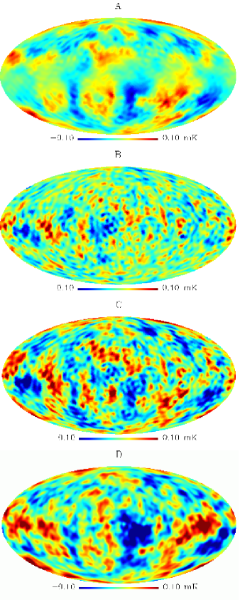
Figure 2: Reconstructed signal maps in Galactic coordinates. A: The posterior mean signal map ($\int dssP(s|d))$ for the COBE-DMR data. This is a generalized Wiener filter which does not require knowing the signal covariance a priori. B: One sample drawn from the conditional posterior $P(s|C_{l},f,d)$. The posterior mean signal map, shown in panel A, has been removed. C: The sample pure signal sky at the same iteration. This is the pixel-by-pixel sum of the maps in panels A and B. D: The WMAP data smoothed to 5 degrees (less than A, more than C). The corresponding features in parts A and D are clearly visible.

IV Example Applications to the Cosmic Microwave Background

In the online materials for this talk (see footnote 1) I present the results of applying the MAGIC method to a synthetic data set which covers an unsymmetrically shaped part on the celestial sphere. I used MAGIC to reconstruct the signal on the full sky and to make movies of the Gibbs sampler iterations. This is an example where the signal is automatically discovered in the data by the algorithm, without specification of the signal covariance.

Figures 2 and 3 show the results of analyzing the COBE-DMR data COBE , one of the most analyzed astronomical data sets. This allowed us to perform consistency checks between the MAGIC method, other methods and the recent results from the Wilkinson Microwave Anisotropy Probe (WMAP) WMAP .

Figure 3: Marginal posterior densities for each individual $C_{\ell}$ from the COBE-DMR data. At each $\ell$ the fluctuations in the $C_{\ell}$ at all other $\ell$ were integrated out. The axis ranges are the same for all panels.

I am also very interested in evaluating claims that the WMAP data favors theories which predict a lack of large scale fluctuation power in the CMB. This claim, if true, would have far-reaching consequences for our understanding of the Universe. Since cosmologists only have one sky to study, we have to be very careful to account for our limited ability to know the ensemble averaged power spectrum on large scales. The WMAP team estimated the fluctuation power on large scales using several techniques and consistently found it to be low. However, in all of these techniques, the variance of the estimates was computed in an approximate way (e.g. in terms of the curvature at the peak) and relies on theory for the assessment of statistical significance. Using MAGIC one can easily integrate over the posterior density of the power spectrum given the data. Therefore it is easy to compute the probability for the power spectrum coefficients in any given $l$-range to be smaller than any given value.

Using the MAGIC method it was straightforward to generate a preliminary sample of the power spectrum coefficients from the WMAP posterior using only the W1 channel, one of the cleanest channels in the WMAP data, in terms of systematic error estimates. For the cleaned W1 data and masking regions of galactic emission (mask Kp0 in the WMAP data release) the quadrupole and octopole power is not obviously discrepant from theoretical expectations. Choosing a more aggressive mask could change this since that reduces the sampling variance. One should bear in mind that the power spectrum likelihood $P(C_{l}|d)$ has infinite variance for $l=2$ even for perfect all-sky data, unless a prior is put on $C_{2}$’s value. Therefore, in an exact assessment of the quadrupole issue claims of a significant discrepancy ought to be based on the actual shapes of posterior density, not a chi-square test (compare the detailed discussion of cosmic variance in MAGIC ). I will address the issue of low power in the low cosmological multipoles in a future publication.

V Future Directions

Of course, if desired, additional prior information about our Universe can be added to the analysis. For example instead of viewing the power spectrum as the quantity of interest, its shape could be parameterized as a function of the $\sim 10$ cosmological parameters which span the space of cosmological theories. Then instead of sampling from the power spectrum coefficients given the signal, one would run a short Metropolis-Hastings Markov chain at each Gibbs iteration to obtain a sample from the space of cosmological parameters given the data. These parameter samples, in turn define a density over the space of power spectra with considerably tighter error bars. The result is the non-linearly optimal filter for reconstructing the mean of the power spectrum incorporating physical information about the origin of the CMB anisotropies.

Another important direction is the analysis of image distortions. The treatment as detailed so far does not allow for the CMB to be lensed gravitationally by the mass distribution through which it streams on its way to us. This distortion itself contains very valuable cosmological information. Extending the formalism to account for lensing of the CMB and estimate the statistical properties of the lensing masses from the lensed CMB would be an important extension of this approach.

- (1) Wandelt, B.D., Larson, D., and Lakshminarayanan, A., astro-ph/0310080, PRD submitted.
- (2) N. Wiener, “Extrapolation, Interpolation, and Smoothing of StationaryTime Series with Engineering Applications,” MIT Press, Cambridge, MA,1949.
- (3) G. B. Rybicki and W. H. Press, “Interpolation, Realization, andReconstruction of Noisy, Irregularly Sampled Data,” ApJ 398, 169 (1992)
- (4) M. Tegmark, Phys. Rev. D55, 5895 (1997)
- (5) J. R. Bond, A. H. Jaffe, and L. Knox, Physical Review D 57, 2117 (1998)
- (6) J. R. Bond, A. H. Jaffe, and L. Knox, Astrophys. J. 533, 19 (2000)
- (7) L. Verde, et al., Ap.J.Suppl. 148, 195 (2003)
- (8) Lewis, A., astro-ph/0310186
- (9) William H. Press, et al., Numerical recipes, Cambridge University Press, Cambridge, UK. (1992)
- (10) Tanner, Tools for Statistical Inference: Methods for the Exploration of Posterior Distributions and Likelihood Functions, Springer Verlag, Heidelberg, Germany. (1996)
- (11) C. L. Bennett et al., Ap. J. 464, L1 (1996)
- (12) C. L. Bennett et al., Ap.J.Suppl. 148, 1 (2003)