Distribution of magnetically confined circumstellar matter in oblique rotators

Abstract

We consider the mechanical equilibrium and stability of matter trapped in the magnetosphere of a rapidly rotating star. Assuming a dipolar magnetic field and arbitrary inclination of the magnetic axis with respect to the axis of rotation we find stable equilibrium positions a) in a (warped) disk roughly aligned with the magnetic equatorial plane and b) at two locations above and below the disk, whose distance from the star increases with decreasing inclination angle between dipole and rotation axis. The distribution of matter is not strongly affected by allowing for a spatial offset of the magnetic dipole. These results provide a possible explanation for some observations of corotating localized mass concentrations in hot magnetic stars.

1 Introduction

Spectroscopic observations indicate the presence of corotating circumstellar matter around chemically peculiar stars (helium-strong, helium-weak, and Ap/Bp stars) with strong magnetic fields (e.g., Shore & Adelman 1981, Walborn 1982, Shore et al. 1990, Groote & Hunger 1997, Smith et al. 1998, Smith 2001). Such accumulation of mass often coexists with magnetically confined outflows (Barker et al. 1982, Brown et al. 1985, Shore et al. 1987, Smith & Groote 2001). Shore and Brown (1990, see also Shore 1987) suggested that the corotating plasma is trapped in a magnetically closed region near the magnetic equator while the stellar wind forms jet-like outflows along open field lines around the magnetic poles. This is similar to the earlier concept of Mestel (1968, see also Mestel & Spruit 1987) of ‘dead zones’ and ‘wind zones’ and also reminiscent to the structure of the solar corona during activity minimum (e.g., Pneuman & Kopp 1971). Recently, Ud-Doula & Owocki (2002) have carried out two-dimensional MHD simulations illustrating the development of open and closed field topologies around a non-rotating hot star with a line-driven wind.

A mechanism for the accumulation of circumstellar matter in equatorial disks around Be stars has been proposed by Bjorkman & Cassinelli (1993, see also Cassinelli et al. 2002, and references therein). They suggest that the strong magnetic field forces the radiatively driven outflowing matter to follow the dipolar field lines and collide near the magnetic equator. Since the colliding flows are supersonic, shock heating leads to UV and X-ray emission. After the material has cooled sufficiently, it accumulates near the magnetic equator and forms a disk. Babel and Montmerle (1997) have proposed a similar mechanism for corotating circumstellar matter and X-ray emission from Ap/Bp stars. For the matter to become magnetically trapped in a closed part of the magnetosphere, the kinetic energy density of the wind has to be smaller than the magnetic energy density. Depending on the strength of the magnetic field, wind speed and mass loss rate, estimates yield an extension of the corotating magnetosphere of up to 10 stellar radii.

Most of the previous theoretical considerations of the equilibrium and dynamics of circumstellar matter around magnetic stars considered aligned rotators, for which the magnetic axis and the rotation axis coincide. In this case, the trapped matter accumulates near the equatorial plane. The distribution of the magnetospheric matter in an oblique rotator with arbitrary relative inclination of the two axes is far less clear. Here we consider this general case by studying the force equilibrium and the stability of circumstellar matter in the closed magnetosphere of an oblique rotator. Assuming that the magnetic energy density is much larger than the kinetic energy density of rotation, which, in turn, is much larger than the thermal energy density of the plasma, we can assume the magnetic field to be fixed and ignore the thermal pressure. The equilibrium problem is then reduced to finding the locations where the (vector) sum of the gravitational and the centrifugal force is perpendicular to a given magnetic field line. A similar approach has been taken by Nakajima (1985), who considered the minima of the effective potential energy along a given magnetic field line. Nakajima apparently determined the absolute minima of the potential and thus could only find one equilibrium locus per field line. In our work, however, we show that there are more locations where the trapped plasma can accumulate. We thus are able to predict the complete spatial distribution of the magnetospheric plasma in a rapidly rotating magnetic star.

The paper is organized as follows. Sec. 2 describes the method to determine the force equilibrium and its stability. Sec. 3 gives results for the special cases of aligned and perpendicular rotators as well as for other relative inclinations of the rotation and magnetic axes. We also consider offset dipoles. We discuss the results in Sec. 4 and present our conclusions in Sec. 5.

2 Force equilibrium and stability

We consider the closed part of the magnetosphere of a rapidly rotating star, i.e., the region inside the Alfvén radius defined by the equality of stellar wind speed and Alfvén velocity. We assume the scaling

$$v^{2}_{\rm s}\ll v^{2}_{\Omega}\ll v^{2}_{\rm A}\,,$$ (1)

where $v_{\rm s}$, $v_{\Omega}$, and $v_{\rm A}$ are the local sound speed, rotational speed (in an inertial frame), and Alfvén speed, respectively. This scaling corresponds to a situation where the magnetic energy density is much larger than the kinetic energy density of the rotational motion, which, in turn, is much larger than the thermal energy density of the magnetospheric matter. Under these conditions, which are relevant for the observed stellar magnetospheres out to about 10 stellar radii (Nakajima 1985; Shore 1987; Babel & Montmerle 1997), the magnetic field is largely unaffected by the presence of circumstellar matter. In the limit of very large electrical conductivity, the gas is attached to the magnetic field lines and the distribution of the circumstellar matter along a given field line is determined by the gravitational and the centrifugal forces (in a corotating frame of reference). Since under the scaling given by Eq. (1) the field lines are practically rigid (a minimal distortion of the field can balance any force perpendicular to the field lines), the force equilibrium for a mass element $\delta m$ is given by the balance of the components of the gravitational and centrifugal forces tangential to the local field line,

$$({\bf F}_{\rm C}+{\bf F}_{\rm G})\cdot{\bf B}=0\;,$$ (2)

where ${\bf B}$ is the magnetic field vector,

$${\bf F}_{\rm C}=\delta m\,\,\Omega^{2}r\;\left[{\bf e}_{r}-{\bf e}_{\Omega}\,({\bf e}_{r}\cdot{\bf e}_{\Omega})\right]$$ (3)

is the centrifugal force and

$${\bf F}_{\rm G}=-\,G\frac{M\delta m}{r^{2}}\;{\bf e}_{r}$$ (4)

is the gravitational force. Here ${\bf e}_{r}$ denotes the radial unit vector, pointing from the center of the star to the mass element located at a radial distance $r$. ${\bf e}_{\Omega}$ is the unit vector along the axis of rotation, $G$ denotes the gravitational constant and $M$ the mass of the star. We consider a magnetic dipole field with a dipole moment, ${\bf m}$, parallel to the unit vector ${\bf e}_{\rm m}$:

$${\bf B}=\frac{\mu_{0}}{4\pi r^{3}}\;\left[3({\bf e}_{r}\cdot{\bf m}){\bf e}_{r}-{\bf m}\right]\;.$$ (5)

Inserting Eqs. (3) - (5) in Eq. (2) yields

$$\left[{\bf e}_{r}\left(1-\frac{GM}{\Omega^{2}r^{3}}\right)-{\bf e}_{\Omega}\,({\bf e}_{r}\cdot{\bf e}_{\Omega})\right]\cdot\biggr{[}3({\bf e}_{r}\cdot{\bf e}_{\rm m}){\bf e}_{r}-{\bf e}_{\rm m}\biggl{]}=0\;,$$ (6)

which can be written as

$$A\,({\bf e}_{r}\cdot{\bf e}_{\rm m})+({\bf e}_{r}\cdot{\bf e}_{\Omega})({\bf e}_{\Omega}\cdot{\bf e}_{\rm m})=0\;$$ (7)

with

$$A=2\left(1-\frac{GM}{\Omega^{2}r^{3}}\right)-3({\bf e}_{r}\cdot{\bf e}_{\Omega})^{2}\;.$$ (8)

The quantity ${GM}/{\Omega^{2}r^{3}}$ represents the ratio of the gravitational to the centrifugal force. Kepler rotation would give a value of unity for this quantity. $\left(GM/\Omega^{2}\right)^{1/3}\equiv r_{{\rm co}}$ is thus called the corotation radius.

Eqs. (7) - (8) show that the distribution of the equilibrium positions is scale-invariant for a fixed value of the angle $\psi$ between the magnetic and the rotational axes $({\bf e}_{\Omega}\cdot{\bf e}_{\rm m}=\cos\psi)$. Therefore, writing $r$ in units of $r_{\rm co}$ allows us to obtain the result for any values of the stellar parameters $\Omega$ and $M$ after proper rescaling with $r_{\rm co}$.

To analyse the stability of a mass element located at an equilibrium position ${\bf r}_{0}$ we consider the projection of the total force $({\bf F}={\bf F}_{\rm C}+{\bf F}_{\rm G})$ on the tangent vector ${\bf l}$ of the field line for a small tangential displacement, $\eta$, of a mass element from its equilibrium position along the corresponding magnetic field line. Denoting the equilibrium quantities by a subscript zero and neglecting second- and higher-order contributions in $\eta$, we have

$${\bf F}\cdot{\bf l} = ({\bf F}_{0}+\delta{\bf F})\cdot({\bf l}_{0}+\delta{\bf l})$$

$$= [{\bf F}_{0}+\eta\,({\bf l}_{0}\cdot{\bf\nabla}){\bf F}({\bf r_{0}})]\cdot({\bf l}_{0}+{\bf n}_{0}\,\eta\,\kappa^{-1}_{0})\;,$$

with

$${\bf F}({\bf r}_{0}+\eta\,{\bf l}_{0})={\bf F}_{0}+\eta\,({\bf l}_{0}\cdot{\bf\nabla}){\bf F}({\bf r_{0}})$$ (10)

and

$${\bf l}({\bf r}_{0}+\eta\,{\bf l}_{0}) = {\bf l}_{0}+\eta\,({\bf l}_{0}\cdot\nabla){\bf l}({\bf r}_{0})$$

$$= {\bf l}_{0}+\eta\,\kappa^{-1}_{0}\,{\bf n}_{0}\;.$$

$\kappa_{0}$ is the local curvature radius and ${\bf n}_{0}$ is the normal vector to the field line through ${\bf r}_{0}$. From Eq. (2) we obtain

$${\bf F}\cdot{\bf l}=\left\{\left[({\bf l}_{0}\cdot{\bf\nabla}){\bf F}\right]\cdot{\bf l}_{0}+{\bf F}_{0}\cdot{\bf n}_{0}\,\kappa^{-1}_{0}\right\}\eta$$ (12)

to first order in $\eta$, where we have used the equilibrium condition ${\bf F}_{0}\cdot{\bf l}_{0}=0$. The neccessary and sufficient condition for a stable equilibrium is that the projection of ${\bf F}$ on ${\bf l}$ is directed towards the equilibrium position, viz.

$$\left[({\bf l}_{0}\cdot{\bf\nabla}){\bf F}\right]\cdot{\bf l}_{0}+{\bf F}_{0}\cdot{\bf n}_{0}\,\kappa^{-1}_{0}<0\;.$$ (13)

3 Results

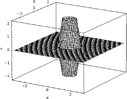
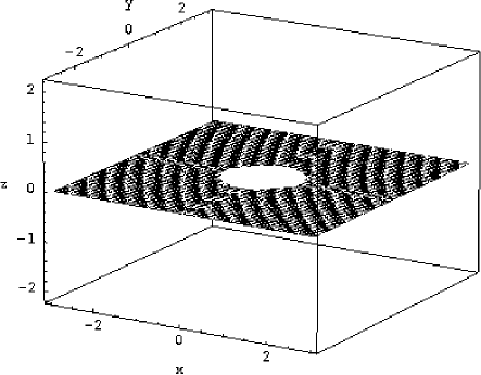
Figure 1: Hatched surfaces show the equilibrium positions for the case $\psi=0$ (aligned rotator) Both the magnetic dipole axis and the rotation axis are in $z$-direction. The left panel shows all equilibrium positions while the right panel shows only the stable ones. All lengths are given in units of the corotation radius.

For the following illustrative examples we use parameter values corresponding to the A0p star IQ Aur (HD 34452, see Babel and Montmerle 1997), namely $M=4.8\,M_{\odot}$, $R_{\star}=5\,R_{\odot}$ and $P_{\rm rot}=2.5\,{\rm d}\rightarrow\Omega=2.9\cdot 10^{-5}\,{\rm s}^{-1}$ and $r_{\rm co}=13.4\,R_{\odot}=2.6\,R_{\star}$. Note that the results for cases with other values of $M$ and $\Omega$ can simply be found by rescaling with the corresponding value of $r_{\rm co}$, so that the results obtained here are, in general, valid for other stellar parameters as well. We first consider the special cases of aligned and perpendicular rotators and then show results for the oblique case.

3.1 Aligned rotator: $\psi=0$

From Eq. (7) we find for the case of parallel rotation and magnetic axes $({\bf e}_{\rm m}\cdot{\bf e}_{\Omega}=1)$ the equilibrium condition

$$\left\{2\left[1-\left(\frac{r_{\rm co}}{r}\right)^{3}\right]-3({\bf e}_{r}\cdot{\bf e}_{\Omega})^{2}+1\right\}({\bf e}_{r}\cdot{\bf e}_{\Omega})=0\;,$$ (14)

with the rotation axis directed along the $z$-axis. This equation has two solutions:

• $\cos\theta\equiv{\bf e}_{r}\cdot{\bf e}_{\Omega}=0$: this solution corresponds to the (coinciding magnetic and rotational) equatorial plane of the star.

• $({\bf e}_{r}\cdot{\bf e}_{\Omega})\neq 0$:

  $$\cos^{2}\theta=1-\frac{2}{3}\;\left(\frac{r_{\rm co}}{r}\right)^{3}$$

The equilibrium locations described by this solution are chimney-shaped surfaces above and below the equatorial plane. This solution only exists for $r\geq(2/3)^{1/3}r_{\rm co}$.

The left panel of Fig. 1 shows all equilibrium locations for the aligned rotator while the right panel gives only the stable equilibria. The ‘chimney’ equilibria are unstable while the equilibria in the equatorial plane are all stable outside the corotation radius.

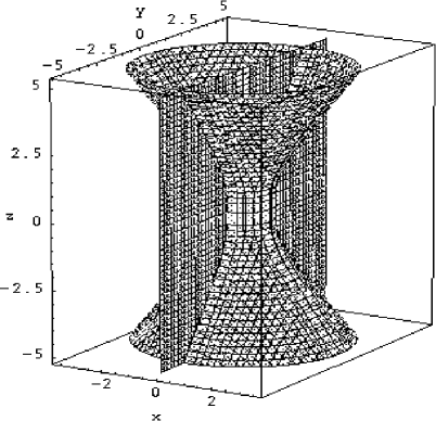
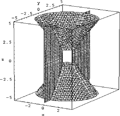
Figure 2: Same as Fig. 1 for the perpendicular rotator ($\psi=\pi/2$). The magnetic dipole is oriented along the $x$-axis.

3.2 Perpendicular rotator: $\psi=\pi/2$

If the rotation axis and the magnetic axis are perpendicular to each other, the equilibrium condition, Eq. (7), becomes

$$\left\{2\left[1-\left(\frac{r_{\rm co}}{r}\right)^{3}\right]-3({\bf e}_{r}\cdot{\bf e}_{\Omega})^{2}\right\}({\bf e}_{r}\cdot{\bf e}_{\rm m})=0\;.$$ (15)

Similar to the previous case, there are two solutions (see Fig. 2):

• ${\bf e}_{r}\cdot{\bf e}_{\rm m}=0$: this solution corresponds to the equatorial plane with respect to the magnetic axis.

• ${\bf e}_{r}\cdot{\bf e}_{\rm m}\neq 0$:

  $$\cos^{2}\theta=\frac{2}{3}\left[1-\left(\frac{r_{\rm co}}{r}\right)^{3}\right]\;.$$

This corresponds to a chimney structure that is axisymmetric with respect to the rotation axis of the star. The solution only exists for $r\geq r_{\rm co}$.

For $r\simeq r_{\rm co}$ the co-latitude $\theta$ is about $90^{\circ}$, corresponding to the base of the chimney at the equatorial plane. For increasing $r$, the co-latitude decreases down to a minimum value of $\theta_{\rm min}=35.3^{\circ}$ (for $r\to\infty$) so that at large distances from the star the chimneys form approximately coni with a constant opening angle $\theta_{\rm min}$.

The stability analysis yields that both equilibrium surfaces are unstable in the close vicinity (out to 1-2 $r_{\rm co}$) but are stable further out.

3.3 Oblique rotators

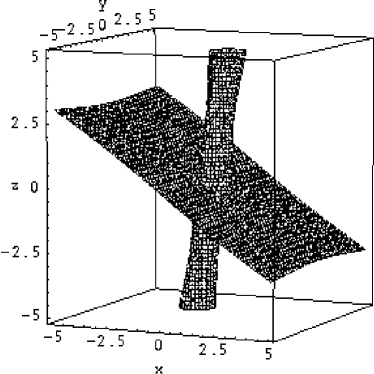
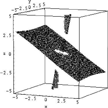
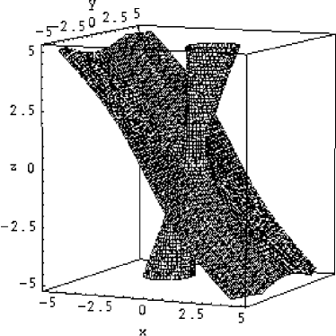
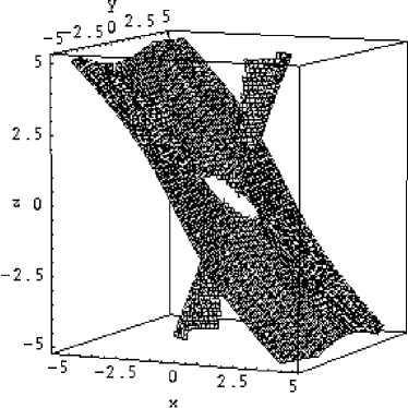
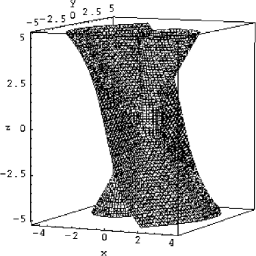
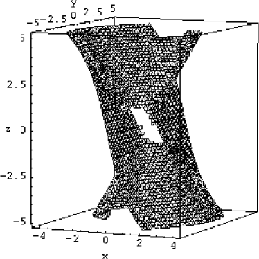
Figure 4: Equilibrium distribution for oblique rotators with various inclination angles (left panels: all equilibrium positions, right panels: only stable positions). Top: $\psi=0.25\pi$, middle: $\psi=0.375\pi$, bottom: $\psi=0.45\pi$. The rotation axis is always oriented along the $z$-axis.

If the inclination angle between the magnetic dipole and the rotation axis is oblique, we have to make use of the complete equilibrium condition, Eq. (7). Again we can find at least two independent solutions which, for small inclinations, describe in good approximation a disk-like and a chimney structure. For larger inclination angle, the shapes of the equilibrium surfaces are modified. This can be seen in Fig. 4 for $\psi=0.25\pi,0.375\pi$, and $0.45\pi$, respectively. For intermediate values, $0\leq\psi\leq 0.5\,\pi$, the disk becomes somewhat warped. In addition to the stable equilibrium points on the warped disk, there are also stable regions on the chimneys. Such regions exist for all values of $\psi$, but they move away from the disk for decreasing inclination and reach infinity for $\psi=0$. The size and the curvature of these regions increases with increasing inclination. They are always completely separated from the disk, exept for the case $\psi=\pi/2$ (Fig. 2) where the disk is directly connected to the stable regions on the chimney. In addition we find that the tilt angle $\theta$ between the stable chimney regions and the rotation axis increases continously from $\sim 0^{\circ}$ for the aligned rotator up to $35.3^{\circ}$ for the case of the perpendicular rotator. This implies that the new stable equilibrium regions can only exist within a specific angular distance from the rotation axis.

The approximate alignment of the (warped) disk-like region of equilibria with the magnetic equatorial plane can be understood by rewriting Eq. (7) in the form

$$\left\{\left[2\left(1-\left(\frac{r_{\rm co}}{r}\right)^{3}\right)-3({\bf e}_{r}\cdot{\bf e}_{\Omega})^{2}\right]{\bf e}_{\rm m}+\cos\psi\;{\bf e}_{\Omega}\right\}\cdot{\bf e}_{r}=0\;.$$ (16)

If the star does not rotate near criticality, we can assume that up to some distance from the stellar surface the term in angular brackets dominates over the second term. In that limit, one solution of Eq. (16) represents the magnetic equator, ${\bf e}_{\rm m}\cdot{\bf e}_{r}=0$. Consequently, for not too rapidly rotating stars, we can always expect an accumulation of matter in the magnetic equatorial plane near to the star. However, the deviation from a flat disk increases for faster rotating stars and is largest in the direction of the tilted dipole. Along these longitudes the disk is always bulged towards the rotational equator.

3.4 Offset dipoles

While we have treated so far only the case of a centered dipole, it appears as if this is more an exception than the rule for the type of stars we consider (e.g., Neiner 2002). A magnetic dipole with an offset vector ${\bf a}$ relative to the center of the star can be written as

$${\bf B}_{\mbox{\tiny{offset}}}=\frac{\mu_{0}}{4\pi\hat{r}^{3}}\;\left[3({\bf e}_{\bf\hat{r}}\cdot{\bf m}){\bf e}_{\bf\hat{r}}-{\bf m}\right]\;,$$ (17)

where ${\bf e}_{\bf\hat{r}}=({\bf r}-{\bf a})/\hat{r}$ and $\hat{r}=|{\bf r}-{\bf a}|$. The equilibrium positions and their stability are determined in full analogy to the case of centered dipoles.

The qualitative behavior of the equilibrium positions for an offset dipole can be seen in Fig. 3 for the case $\psi=0.25\,\pi$ in comparison with the corresponding case with a centered dipole. The stellar parameters are the same as before. In the right panel of Fig. 3 the dipole has been moved by $0.5\,R_{\star}$ along the rotation axis ($z$-axis). The shape of the equilibrium distribution is only slightly modified in comparison to the centered dipole. This is also the case for other realistic offsets (i.e., such that the dipole center remains within the star). Taking into account that we are mainly interested in the large scale distribution of matter $(\sim 5-6\,\,r_{\rm co})$ this result is not surprising since the field geometry on this scale is hardly influenced by dipole shifts $\ll 1\,r_{\rm co}$. Consequently, changes in the equilibrium distribution of circumstellar matter due to reasonable magnetic offsets are almost negligible.

   

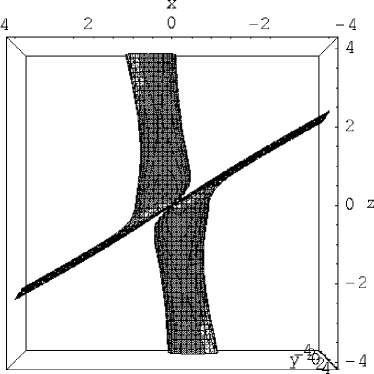
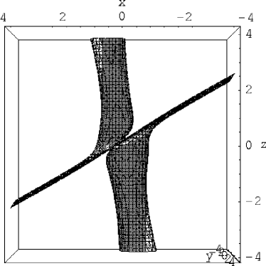
Figure 3: Equilibrium surfaces for inclination angle $\psi=0.25\,\pi$. Left: Centered dipole, right: dipole center displaced by $0.5R_{\star}$ along the rotation axis ($z$-axis). Areas in light and dark gray indicate the stable and unstable equilibrium regions, respectively.

4 Discussion

The origin of corotating circumstellar matter around hot stars with strong magnetic fields is commonly explained with the models of Cassinelli et al. (2002) and Babel & Montmerle (1997) in terms of a radiatively driven stellar wind following the (approximately dipolar) magnetic field lines. Since the material streams from both hemispheres of the stellar surface and reaches supersonic speed, the model suggests that the plasma collides and forms a shock in the magnetic equator. The plasma cools through UV and X-ray emission and accumulates in an equatorial disk. While most of the theoretical calculations assume the special case of aligned magnetic and rotation axes, we have determined the equilibrium plasma distributions for the general case of an oblique dipolar rotator and also determined their stability properties. For aligned magnetic and rotation axes we confirm the accumulation of matter in a circumstellar disk. For increasing inclination angle the disk becomes warped and additional stable equilibrium positions appear. These are curved surfaces, roughly aligned with the axis of rotation, located above and below the magnetic equatorial plane. They grow and move towards the star for increasing values of $\psi$. For the case of a decentered dipole we find that for reasonable offsets the stable equilibrium positions are changed only slightly compared with a centered dipole. We expect that, analogous to the formation of the equatorial disk, the newfound stable equilibrium positions lead to the local accumulation of plasma. Incoming material from the wind is cooled down by radiation behind shocks. Therefore, depending on the kinetic energy of the incoming plasma, we expect that the mass accumulation outside the disk appear in observations of continous and rotationally modulated IR, UV and X-ray emission, which is affected by the size of the emission region and its relative orientation to the line of sight.

In fact, there are observations which indicate the existence of additional equilibrium positions outside the equatorial disk. For the rapidly rotating Be star $\omega$ Orionis, Neiner et al. (2003) found evidence for the presence of two corotating regions of material outside the plane of the disk by measuring variations in the peak intensities of emission lines. Such clouds were also reported by Short & Bolton (1994) for the magnetic He-strong star $\sigma$ Ori E.

We are aware that our model is rather crude. Possible extensions include the dynamics of the radiatively driven wind and the corresponding cooling and accumulation processes. These should be incorporated into three-dimensional MHD simulations in order to understand the dynamics and distribution of plasma in rotating dipolar fields. First steps in this direction are the two-dimensional MHD simulations by Ud-Doula & Owocki (2002) (see also Ud-Doula & Owocki, 2003).

5 Conclusion

A simple consideration of the mechanical equilibrium of plasma in the magnetosphere of a rotating magnetic star with relative inclination of the magnetic and rotation axes suggests the following distribution of matter accumulating, e.g., from a stellar wind:

1. a disk-like structure roughly aligned with the magnetic equatorial plane

2. two locations above and below the disk, coarsely aligned with the axis of rotation.

The latter stable equilibrium regions are most prominent for large obliquity of the axes (perpendicular rotator). They provide hitherto unknown locations for the accumulation of circumstellar matter, which could explain some observations of rapidly rotating magnetic stars, e.g. the close alignment of the new stable regions with the rotation axis could result in an observable rotational modulation of the disk radiation.

We are grateful to Matthias D. Rempel and Francisco Frutos Alfaro for valuable discussions and to Coralie Neiner for pointing us to $\omega$ Orionis and $\sigma$Ori E.
This research has made use of NASA’s Astrophysics Data System Abstract Service.

References

- [1] Babel, J., Montmerle, T., 1997, A&A 323, 121
- [2] Barker, P.K., Brown, D.N., Bolton, C.T., Landstreet, J.D., 1982, In: Advances in Ultraviolet Astronomy, (NASA CP-2238), p.589
- [3] Brown, D. N., Shore, S. N., Sonneborn, G., 1985, AJ 90, 1354
- [4] Cassinelli, J.P., Brown, J.C., Meheswaran, M., Miller, N.A., Telfer, D.C., 2002, ApJ 578, 951
- [5] Groote, D., Hunger, K., 1997, A&A 319, 250
- [6] Mestel, L, 1968, MNRAS 138, 359
- [7] Mestel, L., Spruit, H. C., 1987, MNRAS 226, 57
- [8] Nakajima, R., 1985, Ap&SS 116, 285
- [9] Neiner, C., 2002, Ph.D. Thesis, University of Amsterdam
- [10] Neiner, C., Hubert, A.-M., Frémat, Y., Floquet, M., Jankov, S., Preuss, O., Henrichs, H. F., Zorec, J., 2003, A&A 409, 275
- [11] Pneuman, G. W., Kopp, R. A., 1971, SoPh. 18, 258
- [12] Shore, S.N., Adelman, S.J., 1981, In: The Chemically Peculiar Stars of the Upper Main Sequence (Liége: Institut d’Astrophysique), p.429
- [13] Shore, S.N., Brown, D.N., 1990, ApJ 365, 665
- [14] Shore, S.N., 1987, AJ 94, 731
- [15] Shore, S.N., Brown, D.N., Sonneborn, G., 1987, AJ 94, 737
- [16] Shore, S.N., Brown, D.N., Sonneborn, G., Landstreet, J.D., Bohlender, D.A., 1990, ApJ 348, 242
- [17] Short, C.I., Bolton, C.T., 1994, In: Pulsation; rotation; and mass loss in early-type stars, IAU Symp. 162, Kluwer, Dordrecht, p.171
- [18] Smith, M.A., D. Groote, 2001, A&A 372, 208
- [19] Smith, M.A., Robinson, R.D., Hatzes, A.P., 1998, ApJ 507, 945
- [20] Smith, M.A., 2001, ApJ 562, 998
- [21] Ud-Doula, A., Owocki, S.P., 2002, ApJ 576, 413
- [22] Ud-Doula, A., Owocki, S.P., 2003, In: Proceedings of International Conference on magnetic fields in O, B and A stars, ASP Conference Series, Vol. 216, 1003, (Preprints astro-ph/0310179 and astro-ph/0310180)
- [23] Walborn, N.R., 1982, PASP 94, 322