Formation rate, evolving luminosity function, jet structure, and progenitors for long Gamma-Ray Bursts

Abstract

We constrain the isotropic luminosity function (LF) and formation rate of long $\gamma$-ray bursts (GRBs) by fitting models jointly to both the observed differential peak flux and redshift distributions. We find evidence supporting an evolving LF, where the luminosity scales as (1+z)^δ with an optimal $\delta$ of 1.0$\pm$0.2. For a single power-law LF, the best slope is $\sim$ -1.57 with an upper luminosity of 10^53.3 erg  s^-1, while the best slopes for a double power-law LF are approximately $-1.6$ and $-2.6$ with a break luminosity of 10^52.7 erg  s^-1. Our finding implies a jet model intermediate between the universal structured $\epsilon(\theta)\propto\theta^{-2}$ model and the quasi-universal Gaussian structured model. For the uniform jet model our result is compatible with an angle distribution between 2^∘ and 15^∘. Our best constrained GRB formation rate histories increase from z=0 to z=2 by a factor of $\sim$ 30 and then continue increasing slightly. We connect these histories to that of the cosmic star formation history, and compare with observational inferences up to z$\sim$6. GRBs could be tracing the cosmic rates of both the normal and obscured star formation regimes. We estimate a current GRB event rate in the Milky Way of $\sim 5\ 10^{-5}$ yr^-1, and compare it with the birthrate of massive close WR+BH binaries with orbital periods of hours. The agreement is rather good suggesting that these systems could be the progenitors of the long GRBs.

1. Introduction

The finding of the luminosity function (LF) and formation rate history (FRH) of long $\gamma$-ray bursts (GRBs) is a key issue to understand the nature of these events, as well as to use them as potential tracers of the star formation rate (SFR) in the universe. The most direct way to infer both the LF and FRH is based on the observational luminosity-redshift diagram (LZD) (Schaefer, Deng & Band 2001; Lloyd-Ronning, Fryer & Ramirez-Ruiz 2002; Yonetoku et al. 2003). However, this strategy is conditioned by (i) the bias introduced on the sample by the redshift inference method, and (ii) the sensitivity limit related to the redshift estimate, which in current LZDs is $>1$ photons cm^-2 s^-1. In order to find a reasonable LF, this limit has to be pushed down at least by an order of magnitude. These goals will be reached by future space missions; for example, the Burst Alert Telescope, BAT on-board Swift will be 5 times more sensitive than BATSE, reaching a limiting flux of 10^-8 erg cm^-2 s^-1. Another approach, commonly used in the past, is based on fitting models with parametric LFs and with a given FRH to the observed peak flux GRB distribution, for which the statistics is healthy (see Stern et al. 2002a, and Guetta, Piran & Waxman 2003, and more references therein). Nevertheless, the complicated mixing between the model LF and FRH introduces a degeneracy among these factors in the flux distribution (e.g., Krumhol, Thorsett & Harrison 1998). Some early attempts to fix extra constraints on the fits by using the information provided by the few GRBs with known redshifts were done by Sethi & Bhargavi (2001), Stern et al. (2002a,b) and Guetta et al. (2003).

Taking into account the difficulties mentioned above, here we propose a new strategy to constrain the GRB LF and FRH from the available observations. We will use the widest sample up to date for the differential peak-flux, P, distribution (the logN-logP diagram, NPD hereafter) (Stern et al. 2002b: SAH02), as well as the differential redshift distribution (the N-z diagram, NZD hereafter) from 220 GRBs inferred from an empirical luminosity-indicator relationship (Fenimore & Ramirez-Ruiz 2000: FR00) or from the sample of 33 GRBs with known redshifts (e.g., see the compilation given in van Putten & Riegenbau 2003: PR03). Then, through Monte-Carlo simulations we will optimize the best LF and FRH models by fitting both distributions (NPD+NZD) simultaneously by an accurate minimum global $\chi^{2}$ criterion.

After the discovery of afterglows for the long GRBs, it was realized that their emitted luminosity should be collimated. The simplest model for the jet implies a uniform energy distribution across the jet and a sharp drop outside $\theta_{j}$, where $\theta_{j}$ is the opening angle related to the observed achromatic break time in the light curves (Rhoads 1997). For those bursts with known redshift, and therefore with known isotropic luminosity L_iso, L_iso$\theta_{j}^{2}$ is nearly constant (Guetta et al. 2003), although its distribution results wider than the one found for E${}_{\rm iso}\theta_{j}^{2}$ (Frail et al. 2001; Bloom, Frail & Kulkarni 2003). A further structured jet model proposes a universal non-uniform energy distribution within the jet, the observed diversity of break times in the light curves being caused by a variation of the viewing angle $\theta_{v}$ (Postnov, Prokhorov & Lipunov 2001; Rossi, Lazzati & Rees 2002; Zhang & Mészáros 2002). Similar to the uniform jet model, at least for an energy distribution per solid angle $\epsilon(\theta_{v})\propto\theta_{v}^{-2}$, it was found that L_iso$\theta_{v}^{2}$ is also roughly constant. An alternative approach supposes a Gaussian energy distribution with angle (Zhang & Mészáros 2002; Kumar & Granot 2003). Thus, the origin of the isotropic LF of GRBs could be due in large part to the diversity of opening or viewing angles. Therefore, any improvement on the LF knowledge means a progress on the understanding and constraining of the jet structure (e.g., Guetta et al. 2003; Nakar, Granot & Guetta 2003).

The collimation of the luminosity is also important at the time to calculate the enhancement factor between the observed and the true event rates of GRBs. The enhancement factor for the uniform jet model has been estimated previously to be $<$500 (Frail et al. 2001; PR03), while for the structured jet model, values smaller by more than an order of magnitude were obtained (Zhang et al. 2003; Guetta et al. 2003). Guetta et al. (2003) have also found a small value for this factor ($75\pm 25$) in the case of the uniform jet model. Unlike Frail et al., Guetta et al. used a weighted average of the angular distribution.

An ultimate goal of astronomical studies on GRBs is the connection of the GRB FRH to the SFRH in the universe. Several pieces of evidence show that long GRBs are associated to the core collapse of massive stars. Since the detected $\gamma$-ray fluxes may come from very high-redshifts and from dust enshrouded media, GRBs may offer an interesting way to explore massive star formation in galaxies without the uncertainties of dust extinction, as well as in the universe up to very high redshifts (e.g., Totani 1999; Wijers et al. 1998; Lamb & Reichart 2000; Blain & Natarajan 2000; Ramirez-Ruiz, Threntan & Blain 2002; Choudhury & Srianand 2002; Bromm & Loeb 2002).

Here we will attempt to constrain the GRB FRH by using both the NPD and NZD, and devoting special attention to the behavior at z$>$2. We will also make use of our results to explore the nature of the GRB progenitors. The association of long GRBs to SNIb/c narrows the diversity of potential progenitors to massive helium (Wolf-Rayet, WR) stars, which, owing to the angular momentum requirement, should be in a close binary system with a compact companion. An important task is to estimate the birthrate of these systems in the Milky Way and compare it with the birthrate inferred for the GRBs.

In §2 we describe the observational data that will be used in our study. In §3 the model and strategy applied to constrain the LF and FRH from observations are described. In §4, results regarding the best fitting LFs and FRHs are presented; evolving LFs are strongly favored, and the FRH shape is found to be topologically similar to the global SFR history (SFRH). In §5 we discuss the implications of an evolving LF on current jet models, while in §6 the connection between GRB FR and SFR, and some implications for the progenitors are discussed. Finally, our conclusions are given in §7. Throughout this paper we use the flat $\Lambda$CDM cosmology with $\Omega_{m}$=0.29, $\Omega_{\Lambda}$=0.71, h=0.71.

2. The Data

Stern et al. (2001,2002a) have processed a sample of 3255 BATSE triggered and non-triggered GRBs longer than 1 s. By using an appropriate efficiency matrix they were able to extend the peak flux limit down to 0.1 photons cm^-2 s^-1. In order to extend the flux distribution in the bright side, the data from Ulysses satellite have been used by SAH02 by doing a cross-calibration of the joint Ulysses/BATSE events. The final result is the differential peak-flux distribution corrected by a joint Ulysses/BATSE exposure factor that extends from P=0.1 to about 300 photons cm^-2 s^-1. This is the NPD that we use here (kindly made available in electronic form to us by B.E. Stern). In some previous works, the cumulative P distribution has been used. As noticed by the referee, random errors in a cumulative distribution propagate in an unknown way, therefore for the analysis we pretend to do, the differential distribution should be used.

For the differential redshift distribution we use two samples. The first one is a set of 220 BATSE GRBs with a sensitivity threshold of 1.5 photons cm^-2 s^-1 and with redshifts inferred by using the luminosity-variability empirical relation derived by FR00 (kindly made available in electronic form to us by E. Ramirez-Ruiz). The second sample is a set of 33 GRBs with known z taken from PR03 (excluding GRB980425 and adding GRB030429). This sample is highly biased by selection effects. We attempt to correct some of these effects following Bloom (2003). We use the probability of redshift detection due to observability of lines in the spectral range and in the presence of night-sky lines estimated by Bloom (2003) (who is kindly acknowledged by making available for us an electronic table with the probabilities). The effects related to the distance are accounted with another probability which we set equal to 1 for z$\leq$ 1 and decreasing as 1/(1+z) for larger redshifts (see Gou et al. 2003 for the flux detection of GRB afterglows located at different redshifts).

3. The Model

The differential NPD is modeled by seeding a large number of GRBs with a given FR, $\dot{\rho}_{\rm GRB}$ (per unit of comoving volume), and LF, $f$(L_iso)dL_iso, and by propagating the flux of each source to the present epoch. The rate of GRBs observed with peak fluxes between P₁ and P₂ is ($\propto$ NPD):

$${\rm\dot{N}(P_{1},P_{2})=\int_{0}^{\infty}dz\frac{dV(z)}{dz}\frac{\dot{\rho}_{GRB}(z)}{1+z}\int_{L_{1}}^{L_{2}}\mbox{$f$(L${}_{\rm iso}$)dL${}_{\rm iso}$}},$$ (1)

with L₁=L_iso(P₁,z) and L₂=L_iso(P₂,z), while the rate of GRBs observed between z₁ and z₂ ($\propto$ NZD) with a limiting sensitivity P_min is:

$${\rm\dot{N}({z_{1}},{z_{2}})=\int_{z_{1}}^{z_{2}}dz\frac{dV(z)}{dz}\frac{\dot{\rho}_{GRB}(z)}{1+z}\int_{L_{m}}^{\infty}\mbox{$f$(L${}_{\rm iso}$)dL${}_{\rm iso}$}},$$ (2)

where L_m=L_iso(P_min,z), dV(z)/dz is the comoving volume at z, the term 1/(1+z) takes care of time dilation, and L_iso(P,z) is obtained by solving the equation:

$${\rm P=\frac{(1+z)\int_{(1+z)E_{min}}^{(1+z)E_{max}}S(E)dE}{4{\pi}d_{L}^{2}(z)}},$$ (3)

where E_min=50 keV and E_max=300 keV define the sensitivity band, S(E) is the source differential rest-frame photon luminosity, and d_L(z) is the luminosity distance (see Porciani & Madau 2000). L_iso in the rest frame is defined as L_iso=$\int_{\rm 30keV}^{\rm 10000keV}$ES(E)dE. For the spectrum, we use the Band et al. (1993) proposed fit to a sample of BATSE spectra, with the parameters taken from averages re-derived by Preece et al. (2000) ($\alpha=-1$, $\beta=-2.25$, E$\rm{}_{b}=256$ keV). Notice that these values are in the observer rest frame. It is assumed that the shape of the Band et al. spectrum does not change with z. In the assumption that the average redshift of the GRB sample used here is z=1, E_b would be 511 keV (Porciani & Madau 2000).

Recently it was discovered a relation between the observed peak energy in the spectrum (related to E_b) and L_iso (Yonetoku et al. 2003; see Amati et al. 2002 and Lamb, Donaghy & Graziani 2003 for the analogous correlation between E_b and E_iso). We will explore both cases, a rest E_b constant and a rest

$${\rm E_{b}\simeq 15\ (\mbox{L${}_{\rm iso}$}/10^{50}\ \mbox{erg \ s${}^{-1}$})^{0.5}\ keV}.$$ (4)

Once defined the cosmological model, the LF, and the FRH, then we calculate the NPD and NZD trough Monte-Carlo simulations. We use a single power law (SPL) LF,

$$f(\mbox{L${}_{\rm iso}$})\propto\mbox{L${}_{\rm iso}$}^{-\gamma},\ \ \ \ \ \ \ {\rm L_{l}<\mbox{L${}_{\rm iso}$}<L_{u}},$$ (5)

supported by several theoretical models, or a double power law (DPL) LF:

$$f(\mbox{L${}_{\rm iso}$})\propto\left\{\begin{array}[]{ll}\mbox{L${}_{\rm iso}$}^{-\gamma_{1}},&\mbox{$\ \ \rm L_{l}<\mbox{L${}_{\rm iso}$}<L_{b}$}\\ \\ \mbox{L${}_{\rm iso}$}^{-\gamma_{2}},&\mbox{$\ \ \rm L_{b}<\mbox{L${}_{\rm iso}$}<L_{u}$}\end{array}\right.$$ (6)

suggested by several studies (e.g., Schmidt 1999,2001; FR00; Schaefer et al. 2001; SAH02). From a statistical analysis of a sample of GRBs with z and L_iso inferred from empirical luminosity-estimator relationships, Lloyd-Ronning et al. (2002) and Yonetoku et al. (2003), have suggested that the luminosity should scale with redshift as (1+z)^δ, with $\delta\approx$1.4 and 1.9, respectively.

The GRB FRH per unit of comoving volume is given by:

$${\rm\dot{\rho}_{GRB}=K\dot{\rho}_{SF}},$$ (7)

where $\dot{\rho}_{\rm SF}$ is the GRB FRH normalized to a level close to the one of cosmic SFRH, and defined as:

$${\dot{\rho}_{\rm SF}={\eta}({\rm z})\ \frac{0.3\ e^{b{\rm z}}}{e^{b{\rm z}}+a}\ \mbox{M${}_{\sun}$Mpc${}^{-3}$yr${}^{-1}$}}.$$ (8)

From observations of cosmic SFRH, Porciani & Madau (2001) fit $a=22$ and $b=3.4$. Varying $a$, this equation allows to study the effects of the SFR decline from z=2 to 0. The function $\eta$(z)=1 for z$<$2, and $\eta$(z)=e^c(z-2) for z$>$2, allows to study the effects of a growth (decline) of $\dot{\rho}_{\rm SF}$ for z$>$2 depending on the value of $c>0$ ($c<0$). Notice that the factor K gives information on the GRB progenitor FR and has unities of $\mbox{M${}_{\odot}$}^{-1}$.

The strategy is to constrain the LF parameters ($\gamma$,L_u) for SPL (keeping L_l=10⁴⁹ erg  s^-1), and ($\gamma_{1}$, L_b, $\gamma_{2}$) for DPL (keeping L_l=10⁴⁹ erg  s^-1 and L_u=10⁵⁵ erg  s^-1), as well as the $a,\ b,\ c,\ \delta$, and K parameters. The constraints will be obtained by a joint fit of the model predictions to the observed NPD and NZD (including their errors), using a global $\chi^{2}$ criterion. The total $\chi^{2}$ is the sum of $\chi_{\rm NP}^{2}$ and $\chi_{\rm NZ}^{2}$. In order to verify the quality of fit, tests have been made assuming the total $\chi^{2}$ to be a linear combination of $\chi_{\rm NP}^{2}$ and $\chi_{\rm NZ}^{2}$, with weight coefficients that scale inversely to the number of data (bins) in the NPD and NZD samples, respectively, in such a way that each sample conditions the model with the same strength. The parameter optimization is based on the non linear Levemberg-Marquardt method to find the least $\chi^{2}$ (Press et al. 1988). In spite of the large uncertainties, the redshift distribution of 33 GRBs with known z will be also used as a complementary test.

4. Results

We have run several models with a SPL or DPL LF (identified by S an D, respectively), adopting E_b=511 keV or E_b as a function of L_iso according to eq. (4) (Yonetoku et al. 2003; identified by P and Q, respectively), and either without evolution ($\delta=$0) or including $\delta$ among the parameters to optimize (identified by 0 and E, respectively). The parameters of each one of these models were optimized by a simultaneous fit to the observed NPD and NZD samples, as described in §3. Table 1 gives for each model, identified as was specified above, the values of the fitted parameters, where the same symbols of §3 were used. The uncertainties are the conventional standard deviations. The number of degrees of freedom (for the simultaneous fit) corresponding to each models given in Table 1 is 43 minus the number of parameters shown in Table 1 for the corresponding model. The information about the quality of the fit for the models is given in Table 2. For each model, this Table shows the total $\chi^{2}$, the goodness-of-fit test given by the probability Q to find a new total $\chi^{2}$ exceeding the current value, the partial $\chi_{\rm NP}^{2}$ and $\chi_{\rm NZ}^{2}$ as well as the significance levels, $\rm P_{\rm NP}^{\rm KS}$ and $\rm P_{\rm NZ}^{\rm KS}$, of the Kolmogorov-Smirnov test between the fitted distributions and the NPD and NZD samples, respectively. We have introduced the Kolmogorov-Smirnov test just for completeness; in fact, for all the models the obtained values of the significance levels are not sufficiently high as to disprove the null hypothesis that the expected and observed cumulative distributions are from the same parent distribution. Nevertheless, even if these significance levels are affected by noise, they reveal a minor quality of the fit for SP0 and DP0 models as well as an intermediate quality for SQ0 and DQ0 models. The Q probability shows clearly this situation.

In Fig. 1 we plot the observed and the modeled NPD and NZD. The models with SPL and DPL LFs are on top and bottom panels, respectively. Dotted lines are for models without evolution (0), while solid lines are for models with the optimized evolution parameter $\delta$ (E). Thin and thick lines identify the cases P and Q, respectively. The data are the points with error bars from SAH02 (NPD) and from FR00 (NZD).

GRB luminosity function and evolution. The fit of models to the data at the side of the lowest P’s in the NPD fixes the value of the K factor, while the slope here determines the $\gamma$ (SPL) or $\gamma_{1}$ (DPL) LF parameters. The quality of the fit can be estimated actually at intermediate and high P’s. A scale invariant (without cutoff) power law LF should provide a (log-log) NPD close to a straight line because the power index keeps memory in the NPD, while the FRH does not influence on it (e.g., Loredo & Wasserman 1998). Any break to scale invariance introduces some curvature besides of the volume evolution effect. The imprint of the FRH on the NPD becomes more and more significant as the LF diverges from scale invariance. On the other hand, if the LF evolves, then as $\delta$ increases, the LF tends to concentrate again its influence on the NPD, and the curvature in the NPD grows. This is evident in the NPDs of Fig. 1. Non-evolving LFs show a low NPD curvature because L_u or L_b for GRBs at different z spread on a large P range, while for increasing evolutionary effects this spread is reduced and the curvature grows. Finally, it is quite obvious that a reduced range in P (e.g., 1-50 photons cm^-2 s^-1) weakens strongly the condition given by the NPD, and no robust predictions can be made; the range used here is rather large, 0.1-300 photons cm^-2 s^-1. The results regarding non-evolving and evolving LFs are:

1. For both the SPL and DPL cases, the non-evolving LFs fit poorly the data as one may appreciate by the values of the $\chi^{2}$, Q and $\rm P^{\rm KS}$ of Table 2. In the NPD, the non-evolving models show an excess of GRBs at high P, while in the NZD their fits to the data appear by far to be the best ones (Fig. 1). In terms of our comparative analysis, the non-evolving LF can be ruled out.

2. The quality of the fit becomes excellent when an evolving LF is adopted. The evolutionary models indicate an optimal value of $\delta={\rm 1.0}\pm{\rm 0.2}$. Care has to be taken, however, on the fact that the LF is sensitive also to the constraints on the NZD. Therefore, a careful analysis has to be done, using NZDs obtained from samples based on different z determinations, in order to achieve a more conclusive value for $\delta$.

3. The application of our method to the observational NPD and NPZ samples used here points out to a marginal preference of the SPL LF on the DPL LF. For a more conclusive result on this question, an analysis on a complete LZD has to be carried out.

Taking into account these considerations, our preliminary conclusion is that an evolving LF seems to be necessary in order to reproduce both the NPD and NZD.

GRB formation history. The factor K connects the GRB FR (frequency) to the assumed SFR, and it is fixed mainly by the side of low P’s in the NPD. Notice that in Eq. (8), $\dot{\rho}_{\rm SF}$ was normalized to about 0.2 M_☉Mpc^-3yr^-1 at z=2 for most of the models (see Fig. 2); a different normalization would imply an equivalent inverse scaling of K. It is important to remark that the GRB FRH takes into account the contribution of the overall events above L_l at each z (according to the given LF), while in the NZD the lower limit is determined by the sensitivity threshold on P_min. As seen in Fig. 1, the best models in the NZD are those with an evolving LF. Figure 2 shows the SFRHs corresponding to the models of Fig. 1, using the same line code. The vertical segmented area shows the statistical uncertainty of the Q evolving models. The result is encouraging: the GRB FRHs best constrained from observations follow, at least qualitatively, the observed cosmic SFRH up to z$\approx$6 (see §6 and Fig. 4), showing a steep increase from z=0 to z$\sim$2 (a factor of $\sim$30) and a a gentle increasing towards earlier epochs. This result shows the potential usefulness of GRBs as tracers of SFRs at high redshifts. In fact our results suggest some difference among the SFRHs inferred from GRBs and rest-frame UV luminosity (Fig. 4). This difference is expected if the GRB-based SFRH is tracing both normal and obscured SF regimes (see §6).

The effect on the results of assuming whether a constant E_b (case P) or an E_b depending on L_iso according to Eq. (4) (Yonetoku et al. 2003; case Q) is not relevant. For models with a non-evolving LF the fits improve a little when using E_b depending on L_iso, but their quality remain in any case much worse than that of the models with an evolving LF. In our calculations we have assumed, rather arbitrarily, the low luminosity cut-off L_l=10⁴⁹ erg  s^-1. Actually the fit is invariant with respect to a decrease of L_l below $\sim 10^{50}$ erg  s^-1, mainly because the GRBs with lower luminosities appear above the sensitivity limit of 0.1 photons cm^-2 s^-1 in a very reduced volume around the observer. The only fitting parameter that changes with L_l is K, which scales as L${}_{\rm l}^{-0.6}$ for the best models. The highest correlation between the parameters appears between Loga and b, for which the Pearson’s correlation coefficient is 0.85 and $\Delta$Loga $\approx$ 0.4 $\Delta$b.

Finally, we have also carried out our analysis using the NZD from the de-biased sample of 33 GRBs with known redshifts (see §2). Some difficulty derives from the fact that the sensitivity threshold, P_min, of this sample is unknown. Therefore, we have experimented choosing different thresholds between 1 and 5 photons cm^-2 s^-1, and proved that the changes on LF and FRH are not significant. The constrained SFRH and its statistical dispersion are shown in Fig. 2 by the shaded area, assuming P_min=5 photons cm^-2 s^-1, and $\delta=1$. A qualitative agreement with results obtained using the NZD from FR00 is seen. Thus, from different observational samples we reach the same conclusion: the shape of the GRB FRH approximates that one of the cosmic SFRH.

5. Luminosity function and jet models

As mentioned in the introduction, several pieces of evidence suggest that the LF of GRBs could be strongly related to jet collimation effects. From our analysis, using the observed NPD and NZD, we have obtained $\gamma=1.55\pm 0.05$ for the SPL model. This result provides some evidence against the universal structured jet model with $\epsilon(\theta)\propto\theta^{-2}$ (see also Guetta et al. 2003; Nakar et al. 2003), which predicts a differential LF $\propto$L^-2 (Rossi et al. 2002; Zhang & Mészáros 2002), and also against the quasi-universal Gaussian jet structured model, which predicts a differential LF $\propto$L^-1 even if some dispersion of parameter values is allowed (Lloyd–Ronning, Dai & Zhang 2003). Notice, however, that the best slope we have obtained is intermediate between these two cases. In the framework of structured jet models, the low luminosity branch of the LF is testing how the power per unit solid angle behaves for relatively large angles (i.e. corresponding to small apparent luminosities). For power law structured jets, with $\epsilon(\theta)\propto\theta^{-k}$, the predicted LF is a power law with slope $\gamma$=1+2/k (Zhang & Mészáros 2002). Therefore, $\gamma$=1.5 corresponds to k=4, i.e. a steeper value than the “canonical” k=2. This behavior might correspond to the wings of the jet, and not to the entire jet structure: after all, to avoid divergence, $\epsilon(\theta)$ needs to be a much more moderate function of $\theta$ for small $\theta$. Note also that a power law description of $\epsilon(\theta)$ may be an oversimplification of the real case, which could be described instead by a double Gaussian profile (one for the core of the jet and another for the wing, as suggested by the behavior of the GRB 030329 light-curve, Berger et al. 2003a). Also, the unification of GRB and XRF requires $\epsilon(\theta)$ to fall off more steeply than $\theta^{-2}$ at large angles, to not over-produce XRFs (Lamb et al. 2003; Zhang et al. 2003).

For a uniform jet, L_iso=2L₀/$\theta_{j}^{2}$ ($\theta\leq\theta_{j}$) and L_iso=0 ($\theta>\theta_{j}$), being $\theta_{j}$ the beam aperture and L₀ the intrinsic GRB luminosity (Guetta et al. 2003; see also Frail et al. 2001; Bloom et al. 2003). The differential isotropic luminosity distribution scales with $\theta_{j}$ as dN$\propto\theta_{j}^{2}$ dN_j, where dN_j is the differential jet angle distribution. Let assume dN${}_{j}\propto\theta_{j}^{-\nu}$d$\theta_{j}$ and dN$\propto\mbox{L${}_{\rm iso}$}^{-\gamma}$ dL_iso. With some elementary algebra one obtains that $\nu=5-2\gamma$ (see also Guetta et al. 2003). Thus, in the case of the SPL LF the opening angle distribution is: dN_j=0 ($\theta_{j}<{\rm(2L_{0}/L{{}_{u}})^{1/2}}$) and dN${}_{j}\propto\theta_{j}^{-1.9\pm 0.1}$d$\theta_{j}$ ($\theta_{j}\geq{\rm(2L_{0}/L_{u})^{1/2}}$), while in the case of a DPL LF, the opening angle distribution is: dN${}_{j}\propto\theta_{j}^{1.0\pm 1}$ d$\theta_{j}$ ($\theta_{j}<{\rm(2L_{0}/L_{b})^{1/2}}$) and dN${}_{j}=\theta_{j}^{-1.95\pm 0.06}$d$\theta_{j}$ ($\theta_{j}\geq{\rm(2L_{0}/L_{b})^{1/2}}$).

Now, taking into account the bursts of known redshift, peak flux and jet angles (from PR03 and Bloom et al. 2003), at z$\sim$1 we estimate an average value of 2L${}_{0}\sim$0.8 10⁵⁰ erg/s (see Fig. 3) and $\theta_{b}\equiv\ (2L_{0}/L{\rm{}_{b}})^{1/2}\sim$ 2.3^∘. The upper limit $\theta_{u}$ of the jet angle distribution should be determined by the lower limit of LF. This is not our case because of the NPD is not sufficiently extended toward low peak fluxes. Then we adopt an upper limit obtained by the L_iso=${\rm 2L_{0}}/\theta_{j}^{2}$ relation, the Eq. (4), and a low limit E$\rm{}_{b}\sim$ 50 keV on the ground of the BATSE sensitivity. This assumption gives $\theta_{u}\sim$ 15^∘. Based on geometrical considerations, values for $\theta_{u}$ up to 60^∘ cannot be excluded. For the DPL LF case the enhancement factor f${}_{e}=\int$dN_j/$\int$ dN gives f_e=3/$(\theta_{b}\theta_{u})\sim$ 280, the uncertainty being at least a factor two.

Our results suggest a mild luminosity evolution, L_b$\propto$(1+z)^δ with $\delta\sim 1$. We have checked that this luminosity evolution does not contradict the suggestion of a universal energy reservoir for GBRs (Frail et al. 2001). To this end we have calculated the observed peak luminosities of the bursts listed in PR03 using a conversion factor between the listed count rate and flux of 1 count cm^-2 s^-1 = 8.7 10^-8 erg cm^-2 s^-1. For the bursts in common with Bloom et al. 2003), we could then calculate the true peak luminosity using the jet opening angles listed in that paper. Figure 3 shows the jet opening angles and the corresponding true energies, as a function of redshift, for the 24 bursts listed in Bloom et al. (2003). This figure shows also the true luminosity for the 19 GRBs listed both in PR03 and Bloom et al. (2003). For illustration, the dashed line shows the case of an evolution of the true luminosity proportional to (1+z). It is clear that this evolutionary behavior does not contradict the existing data. Note also that the found evolution of the observed luminosity could be associated not to the evolution of the true luminosity, but to the evolution of the aperture angle of the jet.

6. GRBs as tracers of the cosmic Star Formation Rate and implications for the progenitors

The understanding of the SF processes and history is a key issue to integrate a global vision of the universe. GRBs offer the hope of a deep insight of these processes if we will be able to establish a connection between GRBs and stellar evolution. Our results, though still uncertain, have shown that the GRB FRH resembles qualitatively the observed cosmic SFRH. The SFRH traced by the rest-frame UV luminosity and corrected by dust obscuration, as presented in Giavalisco et al. (2004), is shown in Fig. 4. In this figure we plot also our best models from Fig. 2. A significant contribution to the cosmic SFRH could come from sources emitting strongly in the rest-frame far infrared/submillimetre (e.g., Blain et al. 1999; Dunne, Eales & Edmunds 2003). These objects are likely dust enshrouded SF bursts induced by galaxy collisions that follow the major mergers of dark halos at earlier epochs (for a recent review on galaxy formation, see e.g., Firmani & Avila-Reese 2003). GRBs could be direct tracers of the SFRH of these galaxies, although this is still an open question (see e.g., Ramirez-Ruiz et al. 2002; Berger et al. 2003b; Le Floc’h et al. 2003; Barnard et al. 2003).

The possibility that GRBs are tracing also the SFRH in obscured galaxies might explain the apparent differences between the inferred GRB FRH and the observed UV-cosmic SFRH in Fig. 4. Nevertheless, our results are still uncertain due to the nature of the data used to construct the NZD, and are not suitable for a quantitative exploration on these aspects. In the future, when more data will be collected, we hope that the comparison of the SFRHs inferred from luminous SFR tracers and from the GRB FRs will help to clarify interesting questions related to the nature of the GRBs as well as to the SF processes in highly-obscured galaxies and in the high-redshift universe, where reionization makes difficult the observability of typical emission lines associated to SF.

The value of K$\equiv\dot{\rho}_{\rm GRB}/\dot{\rho}_{\rm SF}$ (see Table 1), gives the number of observable (beaming selected) GRB per unit of gas mass transformed into stars. For the preferred models, K$\approx$ 0.5 10^-7 M${}_{\sun}^{-1}$. This value is uncertain because it depends on the assumed $\dot{\rho}_{\rm SF}$ normalization and on the lower LF limit L_l. For a present-day SFR of 4 M_⊙yr^-1 for the Milky Way, we obtain an event rate of $\sim$ 2 10^-7 yr^-1, which should be enhanced by the factor f_e=280 (see §5); the true event rate is then $\sim$ 5 10^-5 yr^-1. This rate is rather uncertain, at least by a factor 2. It is about fifty times lower than the frequency of SNIb/c in the Milky Way, showing that only a small fraction of WR stars exploding as SNIb/c give rise to the GRB phenomenon (see also Podsiadlowski et al. 2004).

Within the framework of the popular collapsar model for long GRBs, the high angular momentum requirement is the main difficulty (e.g., Zhang & Mészáros 2003). In fact, the strong mass loss by the star and the core-to-envelope (dynamo) magnetic coupling slow down the core rotation (Woosley, Zhang & Heger 2002; Spruit 2002; Heger & Woosley 2002; Izzard, Ramirez-Ruiz & Tout 2003). Instead, if the pre-supernova is in a binary system, then the spin-orbit tidal interactions may increase the rotation even to the limit of Kerr black hole (BH) formation after SNIb/c explosion, ensuring a centrifugally supported disk.

Binary systems with a WR star co-rotating with the orbital motion and with a period of hours (which implies a massive BH as the companion) could be the progenitor of long GRBs (Tutukov & Cherepashuk 2003; Tutukov 2003). In fact, the condition for Kerr BH formation is $\omega_{K}R_{K}\sim c$, where $\omega_{K}$, and $R_{K}$ are the angular velocity, and the radius of the formed Kerr BH, respectively, and $c$ is the light speed. If the pre-supernova WR core have an angular velocity $\omega_{C}$ and a radius R_C, then the angular momentum conservation leads to $\omega_{C}$R${}_{C}^{2}\sim\omega_{K}$R${}_{K}^{2}$. Because of the core co-rotation with the orbit motion, $\omega_{C}\approx 2\pi$/P_orbit, then a Kerr BH is produced if cP${}_{\rm orbit}\lesssim$ 2$\pi$R_C(R_C / R_K). If R${}_{C}\sim$ 0.5 R_☉ and R${}_{K}\sim$10⁷ cm, then P${}_{\rm orbit}\lesssim$ 7 hr, while the separation of the binary system, if the total mass $\sim$30M_☉, is $\lesssim$6 R_☉. Close WR+BH binaries show these properties. Such systems exist in nature, and some potential candidates are known, for example Cyg X-3 (WN3-7+ BH) with P_orbit=0.2 days. These GRB progenitor systems might be observed as luminous, massive X-ray binaries.

We can now estimate the FR of massive WR+BH binaries in the Milky Way. Using the initial star-formation function for close binaries (Iben & Tutukov 1984):

$${\rm d^{3}N=0.1\ \Bigl{(}\frac{da_{in}}{a_{in}}\Bigr{)}\ \Bigl{(}\frac{M_{1}}{M_{\odot}}\Bigr{)}^{-2.5}d\Bigl{(}\frac{M_{1}}{\mbox{M${}_{\odot}$}}\Bigr{)}\ dq\ \ {\rm yr}^{-1}},$$ (9)

where a_in is the initial system semi-major axis, M₁ is the initial mass of the primary, and q=M₂/M₁. This function has been determined from observations in the solar neighborhood and implies a roughly uniform distribution of a_in for 10$<$a_in/R${}_{\sun}<$10⁶, a mass distribution of the primaries close to the Salpeter IMF, and a uniform distribution of q. If we adopt M${}_{1}\sim$ 25 M_☉, da_in/a${}_{\rm in}\sim$ 0.5, and dq$\sim$0.3, the estimate of the Kerr BH formation rate in the Milky Way is $\sim$ 10^-4 yr^-1. This rate, whose uncertainty is about a factor 3, corresponds to a population of a few close binary WR progenitors of Kerr BHs at present in the Galaxy. The Kerr BH formation rate derived through the previous purely astronomical arguments matches rather well with the formation rate we have inferred from GRBs. Thus, a self-consistent scenario supports the idea that the GRB progenitors should be close binary massive WR stars, possibly with a massive BH companion.

As well as the SF enshrouded in dense dust clouds, several other effects can influence the shape difference between the GRB FRH and the cosmic SFRH obtained from rest-frame UV luminosity. Metallicity influences the star mass loss and evolution, and consequently the energetic and collimation of GRB. Even the IMF and binary formation function may change with redshift. All these questions should be well understood before using the GRB FR as a tracer of the cosmic SFR.

7. Conclusions

In this work we have exploited the observational peak-flux distribution for more than 3300 GRBs, and the redshift distribution for 220 GRBs inferred from an empirical luminosity-indicator relationship in order to constrain jointly the LF and FRH of long GRBs. Our analysis allows us to draw the following conclusions:

-For single or double power law LFs, the case of non-evolving LF fits poorly the data, while evolving LFs fit rather well both the NPD and NZD. The best fits are obtained for an evolution where luminosity scales as (1+z)^δ, being $\delta={\rm 1.0}\pm{\rm 0.2}$. This evolution increases the probability to observe GRBs from very high redshifts. The introduction of a dependence of L_iso on E_b (Eq. 4) has little effect on the models, the most important one being the improvement of the fit for the models with non-evolving LF. The goodness of the fit of models with both the SPL and DPL evolving LFs are excellent. The quality of the fit for the former is slightly better than for the latter.

-The best models provide a GRB FRH that approximately resembles the observed cosmic SFRH, in particular if the potential contribution of the SFR in the obscured regime is taken into account. The FRH rises steeply from z=0 to z$\sim$2, and then increases gently toward higher redshifts. The results are qualitatively similar when using a sample of 33 GRBs with known z and adequately de-biased from selection effects. More data, in particular in the NZD, are necessary to explore in more detail the connection of GRB FR to the cosmic SFR.

-For the SPL LF, the best slope from the fits is $\gamma=1.57\pm 0.03$. In the understanding that the LF is closely related to collimation effects, this result implies an intermediate case between the universal structured jet model with $\epsilon(\theta)\propto\theta^{-2}$ and the quasi-universal Gaussian structured jet model. For the uniform jet model, the jet angle distributions corresponding to the best model were calculated, giving an indicative range between 2^∘ and 15^∘ at z=1.

-Our best models give a true (after collimation effect correction) GRB FR of $\sim$ 5 10^-5 yr^-1 in the Milky Way. Based on astronomical arguments we have argued that such a FR agrees with that of close binary systems consisting of a WR star and a possible massive BH, with periods of hours. These systems are able to generate a massive Kerr BH after the SNIb/c explosion of the WR (helium) star. The observational counterparts of these potential GRB progenitors should be luminous X-ray binaries (e.g., Cyg X-3), which are estimated to be only a few at present in the Milky Way.

Figure 1.— Top panel: Peak flux differential distribution (NP) with the axis in the top-right part, and redshift differential distribution (NZ) with the axis in the bottom-left part, both for a SPL LF. Error bars show the NP data from SAH02 and the NZ data according to FR00, respectively. Dotted lines are for models without evolution (0), while solid lines are for models (E) with the evolution parameter $\delta$ optimized. Thin and thick lines identify the cases with E_b=511 keV (P) or E_b depending on L_isoaccording to Eq. (4) (case Q), respectively. Dashed straight line is the -3/2 uniform distribution (Euclidean) behavior in the NPD. Bottom panel: Same as in top panel but for a DPL LF.

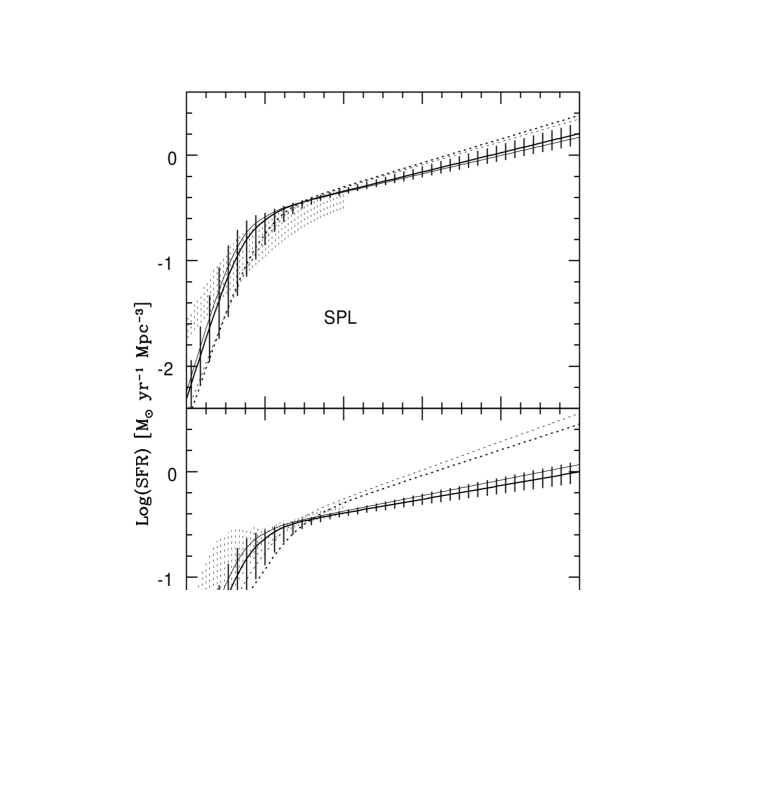
Figure 2.— SFRHs inferred from the GRB FRHs under an opportune normalization. Symbols and models are the same as in Fig. 1. Vertical segmented areas show the 1 $\sigma$ uncertainty for the evolutionary models. Shaded areas show the evolving models, including their uncertainties, for the NZD data corresponding to 33 GRBs with z known (PR03) and de-biased from selection effects.

Figure 3.— From top to bottom: jet opening angle $\theta$, true emitted energy E_true,50 (in units of 10⁵⁰ erg) and true emitted peak luminosity L${}^{\rm peak}_{\rm true,50}$ (in units of $10^{50}$ erg  s^-1), as a function of the redshift z. The values (and limits, for a total of 24 data points) of the jet opening angles and energies are taken from Bloom et al. (2003), while the values from the true luminosities (19 points including limits) have been calculated using the peak count rate of the GRB listed in PR03. In the bottom panel the dashed lines is proportional to (1+z) to show that the mild evolution we find is compatible with existing data and the suggestion of a universal energy reservoir.

Figure 4.— Comparison between the observed cosmic SFRH traced by the rest-frame UV luminosity and corrected by dust obscuration from Giavalisco et al. (2004) (dots with error bars) and the SFRH obtained from GRB FRH opportunely normalized (shaded area). The selected models include the uncertainties and correspond to $\delta$=1, and Eq. (4).

Table 1Best-fit parameters for the LF models

Model	$\gamma$	$\rm LogL_{u}$	Loga	b	c	$\rm\delta$	K
SP0	1.58$\pm$0.04	4.06$\pm$0.07	1.9$\pm$0.2	2.3$\pm$0.4	0.25$\pm$0.04		10.4
SPE	1.53$\pm$0.03	3.3$\pm$0.1	1.7$\pm$0.3	2.7$\pm$0.6	0.20$\pm$0.03	0.9$\pm$0.1	3.43
SQ0	1.59$\pm$0.03	3.96$\pm$0.05	2.0$\pm$0.2	2.5$\pm$0.4	0.26$\pm$0.03		11.6
SQE	1.57$\pm$0.03	3.3$\pm$0.1	1.8$\pm$0.2	2.8$\pm$0.6	0.21$\pm$0.03	0.8$\pm$0.1	4.93

Model	$\gamma_{1}$	$\rm LogL_{b}$	$\gamma_{2}$	Loga	b	c	$\delta$	K
DP0	0.9$\pm$0.4	2.6$\pm$0.3	2.1$\pm$0.2	1.5$\pm$0.4	1.6$\pm$0.6	0.29$\pm$0.05		0.73
DPE	1.53$\pm$0.03	2.8$\pm$0.1	3.4$\pm$0.5	1.6$\pm$0.3	2.8$\pm$0.7	0.17$\pm$0.04	1.2$\pm$0.1	2.85
DQ0	0.8$\pm$0.5	2.4$\pm$0.4	2.1$\pm$0.2	1.8$\pm$0.4	1.8$\pm$0.7	0.28$\pm$0.05		0.78
DQE	1.57$\pm$0.04	2.6$\pm$0.1	2.5$\pm$0.2	1.7$\pm$0.1	2.6$\pm$0.3	0.15$\pm$0.02	1.1$\pm$0.1	4.83

Table 2Statistical quality parameters of the models

Model	$\chi^{2}$	Q	$\chi_{\rm NP}^{2}$	$\chi_{\rm NZ}^{2}$	$\rm P_{\rm NP}^{\rm KS}$	$\rm P_{\rm NZ}^{\rm KS}$
SP0	84.3	2e-5	68.0	16.3	0.46	0.12
SPE	35.7	0.48	26.9	8.8	1e-6	1e-6
SQ0	56.6	0.02	42.8	13.8	3e-3	0.02
SQE	31.7	0.67	24.4	7.4	1e-6	3e-3
DP0	74.6	2e-4	64.3	10.3	0.26	0.02
DPE	35.5	0.44	28.0	7.5	1e-6	5e-5
DQ0	50.0	0.06	39.8	10.2	0.02	4e-3
DQE	36.6	0.40	28.3	8.3	1e-6	5e-5

References

- Amati et al. (2002) Amati, L. et al. 2002, A&A, 390, 81
- Band et al. (1993) Band, D. et al. 1993, 413, 281
- Barnard et al. (2003) Barnard, V.E. et al. 2003, MNRAS, 338, 1
- Berger et al. (2003a) Berger E. et al. 2003a, Nature, 426, 154
- Berger et al. (2003b) Berger E., Cowie, L.L., Kulkarni, S.R., Frail, D.A., Aussel, H. & Barger, A.J. 2003b, ApJ, 588, 99
- Blain & Natarajan (2000) Blain, A.W. & Natarajan, P. 2000, MNRAS, 312, L35
- Blain et al. (1999) Blain, A.W., Smail, I., Ivison, R.J. & Kneib, J.P. 1999, MNRAS, 302, 632
- (8) Bloom, J.S. 2003, AJ, 125, 2865
- Bloom et al. (2003) Bloom, J. S., Frail, D. A. & Kulkarni, S. R. 2003, ApJ, 594, 674
- Bromm & Loeb (2002) Bromm, V. & Loeb, A. 2002, ApJ, 575, 111
- Choudhury & Srianand (2002) Choudhury, T.R. & Srianand, R. 2002, MNRAS, 336, L27
- Dunne et al. (2002) Dunne, L., Eales, S. A. & Edmunds, M. G. 2003, MNRAS, 341, 589
- Fenimore & Ramirez-Ruiz (2000) Fenimore, E. E. & Ramirez-Ruiz, E. 2000, astro-ph/0004176 (FR00)
- Firmani & Avila-Reese (2003) Firmani, C. & Avila-Reese, V. 2003, in “Galaxy Evolution: Theory and Observations”, Eds. V. Avila-Reese et al., RevMexAA (SC), 17, 107
- Frail et al. (2001) Frail, D. A. et al. 2001, ApJ, 562, L55
- Giavalisco et al. (2004) Giavalisco, M. et al. 2004, ApJ, 600, L103
- Gou et al. (2003) Gou, L. J., Mészáros, P., Abel, T. & Zhang, B. 2003, astro-ph/0307489
- Guetta, Piran & Waxman (2003) Guetta, D., Piran, T. & Waxman, E. 2003, astro-ph/0311488
- Heger & Woosley (2003) Heger, A. & Woosley, S.E. 2003, in “Woods Hole GRB meeting”, ed. Roland Vanderspek, AIP Conf.Proc. 662, 214 (astro-ph/0206005)
- Iben & Tutukov (1984) Iben, I. & Tutukov, A.V. 1984, ApJS, 54, 335
- Izzard et al. (2003) Izzard, R.G., Ramirez-Ruiz, E. & Tout, C.A. 2003, MNRAS, in press, astro-ph/0311463
- (22) Kumar, P. & Granot, J. 2003, ApJ, 591, 1075
- (23) Krumholz, M., Thorsett, S.E. & Harrison, F.A. 1998, ApJ, 506, L81
- (24) Lamb, D.Q, & Reichart, D.E. 2000, ApJ, 536, 1
- Lamb et al. (2003) Lamb D.Q., Donaghy T.Q. & Graziani C. 2003, astro-ph/0312634
- Le Floc’h et al. (2003) Le Floc’h, E. et al. 2003, A&A, 400, 499
- Lloyd-Ronning et al. (2002) Lloyd-Ronning, N. M., Fryer, C. L., & Ramirez-Ruiz, E. 2002, ApJ, 574, 554
- Lloyd-Ronning et al. (2003) Lloyd-Ronning N.M., Dai X. & Zhang B. 2003, ApJ, in press, astro–ph/0310431
- (29) Loredo, T.J. & Wassereman, I.M. 1998, ApJ, 502, 75
- Nakar et al. (2003) Nakar, E., Granot, J. & Guetta, D. 2003, astro-ph/0311545
- Podsiadlowski et al. (2001) Podsiadlowski, Ph., Mazzali, P.A., Nomoto, K., Lazzati, D. & Cappellaro, E. 2004, astro-ph/0403399
- Porciani & Madau (2001) Porciani, C. & Madau, P. 2001, ApJ, 548, 522
- Postnov, Prokhorov & Lipunov (2001) Postnov, K.A., Prokhorov, M.E. & Lipunov, V.M. 2001, Astronomy Report, 45, 236
- Preece et al. (2000) Preece, R. D. 2000, ApJS, 126, 19
- Press et al. (1988) Press, W.H., Flannery, B.P., Teukolsky, S.A., & Vetterling, W.T. 1988, Numerical Recipies in C, Cambridge University Press, p. 542
- Ramirez-Ruiz et al. (2002) Ramirez-Ruiz, E., Threntam, N. & Blain, A. W. 2002, MNRAS, 329, 465
- Rhoads (1997) Rhoads, J. E. 1997, ApJ, 487, L1
- Rossi et al. (2002) Rossi, E., Lazzati, D. & Rees, M. J. 2002, MNRAS, 332, 945
- Schaefer et al. (2001) Schaefer, B. E., Deng, M., & Band, D. L. 2001, ApJ, 563, L123
- (40) Sethi, S. & Bhargavi, S.G. 2001, A&A, 376, 10
- Schmidt (1999) Schmidt, M. 1999, ApJ, 523, L117
- Schmidt (2001) ________. 2001 ApJ, 552, 36
- Spruit (2002) Spruit, H.C. 2002, A&A, 381, 923
- Stern et al. (2001) Stern, B. E., Tikhomirova, Ya., Kompaneets, D., Svensson, R. & Poutanen, J. 2001, ApJ, 563, 80
- Stern et al. (2002a) Stern, B. E., Tikhomirova, Ya. & Svensson, R. 2002a, ApJ, 573, 75
- Stern et al. (2002b) Stern, B. E., Atteia, J-L., & Hurley, K. 2002b, ApJ, 578, 304 (SAH02)
- Totani (1997) Totani, T. 1997, ApJ, 486, L71
- Tutukov (2003) Tutukov, A.V. 2003, Astronomy Reports, 47, 637
- Tutukov & Cherapshuk (2003) Tutukov, A.V. & Cherapshuk, A.M. 2003, Astronomy Reports, 47, 386
- van Putten & Regimbau (2003) van Putten, M. P. H. & Regimbau, T. 2003, ApJ, 593, L15 (PR03)
- Wijers et al. (1998) Wijers, R. A. M. J., Bloom, J.S., Bagla, J. S. & Natarajan, P. 1998, MNRAS, 249, L13
- Woosley et al. (2002) Woosley, S.E., Zhang, W. & Heger, A. 2002, in “Woods Hole GRB meeting”, ed. Roland Vanderspek, AIP Conf.Proc. 662, 185 (astro-ph/0206004)
- Yonetoku et al. (2003) Yonetoku, D., Murakami, T., Nakamura, T, Yamazaki, R., Inoue, A.K. & Ioka, K. 2003, astro-ph/0309217
- Zhang & Mészáros (2002) Zhang, B. & Mészáros, P. 2002, ApJ, 571, 876
- Zhang & Mészáros (2003) ________. 2003, Int.Journal Mod.Phys. A, in press, astro-ph/0311321
- Zhang et al. (2003) Zhang, B., Dai, X., Lloyd-Ronning, N.M. & Mészáros, P. 2004, ApJ, 601,L119