GRAVITATIONAL LENSING IN STANDARD AND ALTERNATIVE COSMOLOGIES

GRAVITATIONAL LENSING IN STANDARD AND ALTERNATIVE COSMOLOGIES

DECLARATION

This work has been carried out at the Department of Physics & Astrophysics of the University of Delhi under the supervision of Prof. Daksh Lohiya and Dr. Shobit Mahajan.

The work reported in this thesis is original and it has not been submitted earlier for any degree to any university.

  Margarita Safonova (Candidate)

  Prof. Daksh Lohiya (Supervisor)

  Dr. Shobit Mahajan (Supervisor)

  Prof. K. C. Tripathi (Head of the Department)

List of publications

Published Work

1. M. V. Safonova & D. Lohiya.
   "Gravity balls in induced gravity model—‘gravitational lens’ effects.
   Grav. Cosmol., 6, 327-334 (2000).

2. Margarita Safonova, Diego F. Torres & Gustavo E. Romero.
   "Macrolensing signatures of large-scale violations of the weak energy condition".
   Mod. Phys. Lett. A, 16, 153-162 (2001).

3. Margarita Safonova, Diego F. Torres & Gustavo E. Romero.
   "Microlensing by natural wormholes: theory and simulations".
   Phys. Rev. D., 65, 023001 (2002).

Communicated Work

1. Zafar Turakulov & Margarita Safonova.
   “Motion of a vector particle in a curved space-time. I. Lagrangian approach". Submitted to Mod. Phys. Lett. A. qr-qc/0110067

2. Abha Dev, Margarita Safonova, Deepak Jain, & Daksh Lohiya
   “Cosmological tests for a linear coasting cosmology".
   Submitted to Phys. Letters B. astro-ph/0204150

3. Margarita Safonova & Diego Torres,
   “Degeneracy in exotic gravitational lensing"
   Submitted to Phys. Rev. D., Brief Reports.

Conference Presentations

1. Gravity ball as a possible gravitational lens, Meeting of International Society on General Relativity and Gravitation (GR15), IUCAA, Pune, December 1997.

2. Gravity balls in induced gravity model— ‘gravitational lens’ effects, International Conference on Gravitation and Cosmology, I.I.T. Kharagpur, January 2000.

3. Gravitational lensing as a tool to study alternative cosmologies, 12th Summer School on Astroparticle Physics and Cosmology, ICTP, Trieste, Italy, June 2000.

4. Macrolensing signatures of large-scale violations of a weak energy condition, Young Astronomers Meeting, IUCAA, Pune, January 2001.

5. Energy conditions violations and negative masses in the universe—gravitational lensing signatures, Symposium on Cosmology and Astrophysics, Jamia Milia Islamia, New Delhi, January 2002.

Work in Preparation

1. Zafar Turakulov & Margarita Safonova.
   “Motion of a vector particle in a curved space-time. II. “First order approximation in Schwarzschild  background".

Contents

1. Acknowledgements
2. List of publications
3. 1 General Overview of the Thesis
4. 2 Gravitational Lensing and Its Applications
   1. 2.1 Gravitational lensing as a cosmic telescope
   2. 2.2 Elements of GR and cosmology and propagation of light
      1. 2.2.1 Basic notions of GR
      2. 2.2.2 Weak fields
      3. 2.2.3 Strong fields
      4. 2.2.4 Standard cosmological model
   3. 2.3 Basic concepts of gravitational lensing
      1. 2.3.1 Approximations
      2. 2.3.2 Deflection angle
      3. 2.3.3 Lens equation and the lensing potential
      4. 2.3.4 Magnification
      5. 2.3.5 Lens models
   4. 2.4 Astrophysical applications of gravitational lensing
      1. 2.4.1 Determination of Hubble parameter and mass of the deflector
      2. 2.4.2 A candidate string-lensing field
      3. 2.4.3 Detection of gravitational waves by lensing
      4. 2.4.4 Determination of the lens parameters from gravitationally lensed gamma-ray bursts
      5. 2.4.5 Discovering planetary systems through gravitational microlensing
      6. 2.4.6 Light deflection in strong gravitational fields
5. 3 Gravitational Lensing as a Tool in Search of Natural Wormholes and Negative Matter in the Universe.
   1. 3.1 Introduction
   2. 3.2 Negative mass lensing formalism and basic equations for a point lens
      1. 3.2.1 Effective refractive index of the gravitational field of a negative mass and the deflection angle
      2. 3.2.2 Lensing geometry and lens equation
      3. 3.2.3 Einstein radius and the formation of images
      4. 3.2.4 Time gain and time-offset function
      5. 3.2.5 Magnifications
   3. 3.3 Microlensing
      1. 3.3.1 Light curves of the point source
      2. 3.3.2 Extended sources
      3. 3.3.3 Comments on numerical method and simulations
      4. 3.3.4 Shapes of images and light curves for the uniform brightness source
      5. 3.3.5 Shapes of images and light curves for the sources with non-uniform brightness profiles
      6. 3.3.6 Time scales of microlensing
      7. 3.3.7 Concluding remarks
   4. 3.4 Macrolensing
      1. 3.4.1 Simulations results
      2. 3.4.2 Concluding remarks
6. 4 Gravitational Lensing as a Tool to Test Alternative Cosmologies
   1. 4.1 Introduction
   2. 4.2 Gravitational lensing statistics as a test for coasting cosmology
      1. 4.2.1 Linear coasting cosmology
      2. 4.2.2 Basic equations of gravitational lensing statistics
      3. 4.2.3 Testing the model against observations
      4. 4.2.4 Concluding remarks
   3. 4.3 Gravity balls as gravitational lenses
      1. 4.3.1 Gravity ball as a NTS solution
      2. 4.3.2 Lens model for a G-ball and lensing properties
      3. 4.3.3 Simulations results
      4. 4.3.4 Concluding remarks
7. 5 Propagation of Light in Strong Gravitational Fields
   1. 5.1 Introduction and main motivations
   2. 5.2 Photons in a gravitational field
      1. 5.2.1 Spinning particles
   3. 5.3 Modified geodesic equation for photons
      1. 5.3.1 Theoretical background
      2. 5.3.2 Schwarzschild metric
      3. 5.3.3 The final set of equations
   4. 5.4 Velocity of photons in Kerr metric
      1. 5.4.1 $\epsilon$-matrix
      2. 5.4.2 Kerr metric
   5. 5.5 Derivation of the Papapetrou equation for photons
      1. 5.5.1 Formalism
      2. 5.5.2 Equations of motion
   6. 5.6 Conclusions
8. 6 Summary and Final Comments
9. A Wormhole solution to the Einstein equations
10. B Lensing clusters sample
11. C Full $\epsilon_{i}^{j}$ matrix in $t,\varphi,r,\theta$ components
12. D Structure equations
    1. D.1 Connections
    2. D.2 Derivatives of the components of the frame
13. Bibliography

List of Tables

1. 1 Microlensing time scales for several source radii
2. 1 Lensing cluster sample

List of Figures

1. 2.1 Two-dimensional picture of gravitational lensing situation
2. 2.2 Basic geometry of gravitational lensing
3. 2.3 Lensing by a straight cosmic string
4. 3.1 Embedding diagramme for a wormhole
5. 3.2 Lensing geometry of a negative mass
6. 3.3 Formation of images by a point negative mass lens
7. 3.4 Geometric time delay, gravitational time gain and total time offset produced by a point negative mass lens
8. 3.5 The magnifications for the positive point mass lens and negative point mass lens
9. 3.6 Schematic representation of the geometry of the positive mass lensing
10. 3.7 Schematic representation of the geometry of the microlensing
11. 3.8 True motion of the source and apparent motion of the images for minimum impact parameter $B_{0}>2$
12. 3.9 True motion of the source and apparent motion of the images for $B_{0}=2$
13. 3.10 True motion of the source and apparent motion of the images for $B_{0}<2$
14. 3.11 True motion of the source and apparent motion of the images for $B_{0}=0$
15. 3.12 Light curves for the negative mass lensing of a point source
16. 3.13 Four sets of lens-source configurations for four different values of the dimensionless source radius
17. 3.14 Same as in Fig. 3.13, but for minimum impact parameter $B_{0}=2.0$.
18. 3.15 Image configurations and a corresponding light curve for a Gaussian source
19. 3.16 Same as in the previous Fig. , but with the different effective source radius
20. 3.17 Image configuration for a source with exponential brightness distribution
21. 3.18 Light curves for sources with different brightness profiles
22. 3.19 Appearance of a background field of sources in a range of redshifts for lens mass equal to $1\times 10^{13}\,M_{\odot}$
23. 3.20 Appearance of a background field of sources in a range of redshifts for lens mass equal to $1\times 10^{14}\,M_{\odot}$
24. 3.21 Appearance of a background field of sources in a range of redshifts for lens mass equal to $1\times 10^{15}\,M_{\odot}$
25. 3.22 Appearance of a background field of sources in a range of redshifts for lens mass equal to $1\times 10^{16}\,M_{\odot}$
26. 3.23 Appearance of a background field of sources in a range of redshifts for lens mass equal to $1\times 10^{17}\,M_{\odot}$
27. 3.24 Problems with simulations of a large mass lens
28. 3.25 Problems with simulations of a large mass lens; resolution
29. 3.26 Appearance of a background field of sources at a fixed redshift, lensed by a $1\times 10^{14}\,M_{\odot}$ lens
30. 3.27 Appearance of a background field of sources at a fixed redshift, lensed by a $1\times 10^{16}\,M_{\odot}$ lens
31. 4.1 Predicted number of lensed quasars $n_{\rm L}$ vs. power index $\alpha$
32. 4.2 G-ball as a gravitational lens
33. 4.3 Solution to the lensing equation by a gravity ball
34. 4.4 The magnifications for the gravity ball lensing
35. 4.5 $R_{\rm ball}$ vs. $n$ for different clusters
36. 4.6 Lensing configurations by an empty gravity ball
37. 4.7 Distortion field generated by a simulated gravity ball
38. A.1 Embedding diagrammes for wormholes

Chapter 1 General Overview of the Thesis

This thesis contributes to the field of Gravitational lensing (GL) and observational cosmology. We have investigated the possibility of detecting the existence of matter violating the weak energy conditions through its lensing effect on background sources. In a different context we have investigated GL in an alternative cosmology with a linearly evolving scale factor. We also considered gravitational lensing statistics in such a cosmology and its compatibility with existing observations. We have studied propagation of light in strong gravitational fields and the equations of motion for a vector particle with spin. Using geometrical optics approach we have shown that in Schwarzschild and Kerr geometries, massless particles deviate from geodesic motion.

Einstein’s General Theory of Relativity (GR) predicts that light rays are deviated from their straight path when they pass close to a massive body. This prediction was experimentally verified in 1919. Although the deflection is small, its effect can be enhanced by the passage of light over long distances. The deflected rays have enough time to intersect with one another to form caustics, and for objects which are compact and massive or are at cosmological distances there is a possibility of observing the effects of bending of light. Due to the bending of light, background objects appear distorted and, in extreme cases, form multiple images. This information can be used to obtain the distribution of mass in the lens in a completely novel way. The images of background objects are magnified by the action of lensing which makes them appear bigger (and therefore brighter). Thus, a gravitational lens acts as a natural telescope providing us information about the distant objects which are otherwise too dim to be detected.

GL is a powerful tool for exploring the universe. It can be used for the detection of exotic objects as well as for testing alternative theories of gravity. Proposals have been made to discover cosmic strings, boson stars, neutralino stars or wormholes through their gravitational lensing effects. There is no compelling evidence that any of the observed GL systems are due to these objects. However, it is essential to develop new lens models with objects which are not forbidden on theoretical grounds.

The list of multiple-imaged gravitational lens systems has been growing steadily since the discovery of the first lens system in 1979 (the famous ‘Old Faithful’ QSR 0957+561 A&B). At present, more than 30 multiple-image systems are confirmed, or are very likely to be, as gravitational lens systems. These lens systems can provide us with information about the universe as a whole. The global geometry of the universe, usually specified by its matter density and a cosmological constant, remains a significant source of uncertainty in modern cosmology. The possibility of using GL as a tool for the determination of cosmological parameters, either by a detailed study of specific lensing systems or through statistical analysis of samples of lenses, has been long and frequently discussed. One of the results of the previous works was that the mean image separations of lens systems have different dependence on source redshift in different cosmologies and that it may therefore be possible to measure the curvature of the universe directly. Besides, the expected frequency of multiple image lensing events for high redshift sources turned out to be quite sensitive to some cosmological parameters. All this makes the gravitational lensing statistics an interesting method to test different cosmological models.

CHAPTER TWO is an introduction to the gravitational lensing theory. We give a brief introduction to the basic mathematical formalism for studying gravitational lensing and the background cosmology that we use to describe spacetime in which light propagation takes place. We introduce the terminology and concepts used in GL calculations, and review the basic equations of gravitational lensing. The basic types of lenses are presented and their properties are discussed. The second part of the chapter reviews different astrophysical and cosmological applications of gravitational lensing.

In CHAPTER THREE, the substance of which has appeared as Refs. [1, 2], we discuss the use of gravitational lensing as a tool in search of exotic objects in the Universe. In the first section we give an introduction to the energy conditions (EC) of classical GR and examine the consequences of their possible violations. Typically, observed violations are produced by small quantum systems and are of the order of ${\raise-0.15pt\hbox{$\mkern-0.5mu\barbar$}\mkern-8.5muh}$. One recent experimental study, however reported a violation, which could, in principle, arise because of the existence of classically forbidden regions carrying negative energy. It is currently far from clear whether there could be macroscopic quantities of such an exotic, EC-violating matter.

Of all the systems which would require violations of the EC, wormholes are the most intriguing. The salient feature of these objects is that an embedding of one of their space-like sections in Euclidean space displays two asymptotically flat regions joined by a throat. Since wormholes have to violate the null EC in order to exist, the hypothesis underlying the positive mass theorem no longer applies, and there is nothing, in principle, that can prevent the occurrence of a negative total mass. In other words, we need to have some negative mass near the throat to keep the wormholes open. If wormholes exist, they could have formed naturally in the Big Bang, “inflated" from the “quantum foam" that is thought to underlie spacetime. Alternatively, they could have been constructed by an advanced extraterrestrial civilization as terminuses for, say, pan-galactic subway system.

Discovery of any object with negative mass will not prove the existence of wormholes for sure, although it will certainly enhance the possibilities for wormholes to exist. In this chapter we analyze the gravitational effects light experiences while traversing the regions with negative mass.

In the second section we provide an in-depth study of the theoretical peculiarities that arise in effective negative mass lensing, both for the case of a point mass lens and source, and for extended source situations. We describe novel observational signatures arising in the case of a source lensed by a negative mass. We show that a negative mass lens produces total or partial eclipse of the source in the umbra region and also show that the usual Shapiro time delay is replaced with an equivalent time gain. We describe these features both theoretically, as well as through numerical simulations. In the third section we provide negative mass microlensing simulations for various intensity profiles and discuss the differences between them. The light curves for microlensing events are presented and contrasted with those due to lensing produced by normal matter. Presence or absence of these features in the observed microlensing events can shed light on the existence of natural wormholes in the Universe.

In the last section we present a set of simulations of the macrolensing effects produced by large-scale cosmological violations of the energy conditions. These simulations show how the appearance of a background field of galaxies is affected when lensed by a region with an energy density equivalent to a negative mass ranging from $10^{12}$ to $10^{17}$ solar masses. We compare with the macrolensing results of equal amounts of positive mass, and show that, contrary to the usual case where tangential arc-like structures are expected, there appear radial arcs—runaway filaments—and a central void. These results make the cosmological macrolensing, produced by space-time domains where the weak energy conditions is violated, observationally distinguishable from standard regions. Whether large domains with negative energy density indeed exist in the universe can now be decided by future observations of deep fields.

In the FOURTH CHAPTER we explore GL in an alternative cosmological model and the concordance of this theory with the current gravitational lensing observations. This chapter is divided into three sections. The first section introduces the problems standard model experiences and ways of their resolution. In the second section, part of which has appeared in ref. [3], we investigate the concordance of the gravitational lensing statistics with the cosmology in which the scale factor is linearly evolving. The use of gravitational lensing statistics as a tool for the determination of cosmological parameters either by a detailed study of specific lens systems or through a statistical analysis of a sample of lenses has been frequently discussed. It has been pointed out that the expected frequency of multiple imaging lensing events is sensitive to a cosmology. We use this test to constrain the power index $\alpha$ of the scale factor. We calculate the expected number of multiple image gravitational lens systems in a particular quasar sample with a known distribution of redshifts. This is compared with the observed frequency of lens systems found. Expected number of lens systems depends upon the index $\alpha$ through the angular diameter distances. We derive the expressions for angular diameter distances for this cosmology and use them in the lensing probability functions. By varying $\alpha$, the number of lenses changes, which on comparison with the observations gives us a constraint on $\alpha$. We find that the value $\alpha=1$ corresponding to the coasting cosmology is in concordance with the number of observed lenses in the considered sample. In the last section, substance of which has appeared as ref [4], we introduce the non-minimally coupled effective gravity theory in which one can have non-topological soliton solutions. A typical solution is a spherical region having $G_{\rm eff}=0$ outside, and the canonical Newtonian value inside. Such a spherical domain (gravity-ball) is characterised by an effective index of refraction which causes bending of light incident on it. The gravity ball thus acts as a gravitational lens. We consider the gravity ball to be of a size of a typical cluster of galaxies and show that even empty (without matter) gravity ball can produce arc-like images of the background source galaxy. In the case of background random field the ball produces distortions (‘shear’) of that field. We also obtain constraints on the size of the large gravity ball which can be inferred form the existing observations of clusters with arcs.

The FIFTH CHAPTER is dedicated to studies of the propagation of light in strong gravitational fields. Most cosmological studies of lensing are performed in the weak field approximation. However, there are interesting astrophysical situations where light propagates in a strong gravitational field. Weak field approximation becomes invalid in the vicinity of compact objects like black holes and pulsars. Thus, gravitational lensing can have additional effects. This chapter is divided into 5 sections. In the first two sections we present introduction to the question and motivations for the study. Third section describes the formulations of the theory, where the equation of wave propagation coupled to the curvature of the spacetime is derived. We also derive the modified geodesic equation and present a way to solve the equation. Fourth section discusses the application of the results of the third section to the velocity of photons propagation in the field of the Kerr black hole. We conclude that the velocity remains subluminal contrary to recent claims. Fifth section, an edited version of Ref. [5], is dedicated to another approach to the problem and presents the derivation of the Papapetrou equation for massless particles from a simple Lagrangian.

CHAPTER SIX is the concluding chapter and presents a summary and remarks with directions for the future work.

Some technical details are included in the appendices.

Chapter 2 Gravitational Lensing and Its Applications

2.1 Gravitational lensing as a cosmic telescope

"Do not Bodies act upon Light

at a distance, and by their action

bend its Rays; and is not this action

strongest at the least distance?"

I. Newton, Opticks, 1704

Our Universe is controlled by gravity which doesn’t limit its effects on matter—light rays can be deflected and bent. In 1704 Newton proposed that a light ray passing close to a massive body would be attracted and its path bent. In 1911 Einstein obtained the so-called "Newtonian" value for the deflection angle from the Principle of Equivalence and the undisturbed Euclidean metric. However with the full equations of General Theory of Relativity (GR) Einstein obtained an angle twice the "Newtonian". The 1921 solar eclipse expedition confirmed the “Einstein" value, making the Einstein theory of General Relativity a new paradigm and Einstein famous.

In fact, during those early years many scientists contributed to the subject of light deflection. It is worth mentioning such names as John Michell and H. Cavendish, P. S. Laplace, A. Eddington, who appear to be the first to point out that multiple (double) images can occur if two stars are sufficiently well aligned, O. Chowlson, who is actually responsible for what we now call the "Einstein ring". The first to mention that action of gravity of a massive body on light is similar to the refraction of light in an optical lens and called it "gravitational lens", was a Czech engineer R. Mandl in his letter to Einstein. In 1936 Einstein published a paper about this effect, where he remarked that "there is no great chance of observing this phenomenon". However, in 1937 the famous “prophet" of astrophysics, Fritz Zwicky, published a very optimistic paper about real possibility of discovery of gravitational lens (GL) in case of a galaxy lensed by foreground galaxy. He was the first to point out the usefulness of GL as an astrophysical tool which will allow a deeper look into the universe. He predicted many important applications of GL, pointed out that magnification leads to a selection bias and estimated the probability of detecting lensing to be very high.

In the mid 60’s the discovery of quasars (QSOs) renewed interest in GL. The subject was revived by S. Refsdal, who was later called by R. D. Blanford "the most reliable prophet in gravitational lensing". In his first paper [6] Refsdal gave a full account of the properties of the point-mass GL and calculated the time delay for the two images and mentioned a compact object as a candidate for a lens. In a subsequent paper he considered the application of GL for estimating the mass of the bending galaxy and the Hubble constant through observable parameters of the source-lens system [7]. In 1965 it was suggested by J. Barnothy that QSOs are in fact Seyfert 1 galaxies, made to appear extra bright through other foreground galaxy acting as a gravity lens. It is now believed that QSOs are indeed the nuclei of galaxies, though not especially magnified by GL (with the possible exception of BL Lac objects, that can, in fact, be magnified QSOs). However, only after 1979 when the first GL system (QSO 0957+561 A & B, “The Old Faithful") was discovered did a systematic search for lenses begin. By now many GL systems have been identified which we can roughly divide into three classes: (i) more than 30 proposed multiple images of QSOs; (ii) several tens of arcs and arclets; (iii) several radio and optical rings (and nearly rings) with one possible candidate for an X-ray ring [8]. One can now say that gravitational lensing significantly affects our view and physical understanding of the distant Universe and of its major constituents.

In spite of great theoretical and observational inspiration in GL field, there exist certain problems, as in any other new field. One of the basic problems is the amplification bias. The possible magnification of the source, associated with the deflection, can fool the observer: some QSOs seen through a foreground galaxy are much fainter than they appear to be. If one conducts a flux-limited QSO search, some of these sources get boosted in flux above the threshold of the sample. The net effect is that frequency of multiple imaging appears much greater in flux-limited samples than in volume-limited ones. Another direct consequence of the amplification bias is that one would naturally expect to find an excess of amplifying galaxies near distant and bright QSOs selected from a flux-limited sample. This has indeed been reported [9].

Another problem is the "verification", or "when is a lens a lens". This became important after the discovery of several binary QSOs. There exist several basic characteristics of images that are signatures of gravitational lensing, though this list is by no means exclusive: (i) multiple images of the same object; (ii) background image seen as a nearly complete ring or as an extended arc; (iii) spectroscopic similarities of the images; (iv) detection of the lensing galaxy or cluster in the right location and of sufficient mass to create the image splitting; (iiv) images exhibiting brightness variations characteristic of compact objects crossing the line of sight.

However, in spite of the problems and the uncertainties, the theoretical and observational achievements of last few decades have made the GL one of the most active and exciting fields of research. All possible applications of gravitational lensing are surely impossible to list. From determination of the Hubble constant and mass of the bender to using microlensing for dark matter search to testing alternative gravitation theories and exotic objects search—there is hardly an area of cosmology and astrophysics where GL has not been applied. In this Introduction we will concentrate on the basic theory underlying the gravitational lensing subject and the new progress of GL as well as describe some of its interesting applications in astrophysics.

2.2 Elements of GR and cosmology and propagation of light

2.2.1 Basic notions of GR

The basic principles of Einstein’s GR are considered to be the Principle of Relativity and Principle of Equivalence (EP). However, the decisive step for the construction of the general relativity formalism was the suggestion by Einstein and Grossman in 1912-1913 that the gravitational field must be identified with the non-Minkowskian metric of the spacetime. Usually this suggestion is deduced from the EP. However, some authors consider the metricity of gravitation as the independent, if not, the main, principle of GR [10, 11]. If we accept the metricity of the gravitational field, then a pseudo-Riemannian spacetime must be chosen as the model for our spacetime. (It is characterised by the structure of the manifold, pseudo-Riemannian metric, connection and curvature).

SSDifferential manifold We will assume that the spacetime has the properties of a continuum, i.e. it is a four-dimensional differential affine manifold $X_{4}$. Any point of it can be labeled by real coordinates $x^{\mu}$ with $\mu=0,1,2,3$, where $0$ refers to the time coordinate, and 1,2,3 to the space coordinates. Any affine space has a defined notion of the interval between its points. At any point there exists an independent metric tensor field $g_{\mu\nu}=g_{\mu\nu}(x)$ in order to allow for local measurements of distances and angles. The square of the infinitesimal interval $ds$ between $x^{\mu}$ and $x^{\mu}+dx^{\mu}$ is then determined by

$$ds^{2}=g_{\mu\nu}dx^{\mu}dx^{\nu}\,\,.$$ (2.1)

Thus, we can adopt the definition [12]:
Definition 1 A spacetime is a four-dimensional manifold equipped with a Lorentzian (pseudo-Riemannian ) metric with signature (-,+,+,+). (The manifold should be Hausdorff and paracompact.) This definition is important in the studies of wormholes (see Chapter 3.1). To admit the construction of a wormhole, a spacetime shall be either “almost-everywhere Lorentzian" or be non-Hausdorff. SSConnection In order to do physics in such a spacetime, we should have additional structures on $X_{4}$. In an $X_{4}$ it does not make sense to say “a (nonzero) vector field is constant." To give such a statement a meaning, one must introduce the notion of parallel transfer of vectors. Parallely displaced from $x^{\mu}$ and $x^{\mu}+dx^{\mu}$, a vector $C^{\mu}$ changes according to the prescription

$$dC^{\mu}=-\Gamma^{\mu}_{\alpha\beta}(x){C}^{\alpha}dx^{\beta}\,\,.$$ (2.2)

Here $dC^{\mu}$ is assumed to be bilinear in ${C}^{\alpha}$ and $dx^{\beta}$, the set of the 64 coefficients $\Gamma^{\mu}_{\alpha\beta}$ is the affine connection. An $X_{4}$ equipped with a $\Gamma$ is called a linearly connected space or $L_{4}$. The parallel transport law (2.2) can be extended to higher rank tensor fields and densities, and it is possible to define their covariant differentiation with respect to $\Gamma$; for a vector, $\nabla_{\nu}C^{\mu}=\partial_{\nu}C^{\mu}+\Gamma^{\mu}_{\alpha\nu}C^{\alpha}$. Now it makes sense to state that “a field is constant over spacetime"—its covariant derivative has to vanish. In general, metric and connection are two independent geometrical constructions on a manifold. But in GR, since the gravitational field is identified with the metric, a connection should satisfy two additional conditions:

• Symmetry                                             $\Gamma^{\mu}_{\alpha\nu}=\Gamma^{\mu}_{\nu\alpha}$,

• Metricity                                        $\;\;\;\;\;\;\;\;\nabla_{\nu}g_{\alpha\beta}=0$.

  The last postulate guarantees that lengths, in particular the unit length, and angles are preserved under parallel displacement. This enables a choice of a coordinate system with connection coefficients vanishing at a point $x$ and metric $g_{\mu\nu}(x)=\eta_{\mu\nu}$ (the Minkowskian metric) at this point. Such a coordinate system is called the locally inertial system at $x$.

The above conditions allow us to express the components of such a connection through the metric:

$$\Gamma^{\mu}_{\alpha\nu}=\frac{1}{2}g^{\mu\sigma}\left(g_{\nu\sigma,\alpha}+g_{\alpha\sigma,\nu}-g_{\nu\alpha,\sigma}\right)\,\,.$$ (2.3)

Components (2.3) are called Christoffel symbols. SSCurvature Parallel transfer is a path-dependent concept. If we parallely transfer a vector around an infinitesimal area back to its starting point, we find that its components change. This change is proportional to the Riemann curvature tensor

$$R_{\alpha\beta\gamma}^{\;\;\;\;\;\;\;\;\delta}:=2\partial_{[\alpha}\Gamma^{\delta}_{\beta]\gamma}+2\Gamma^{\delta}_{[\alpha|\sigma}\Gamma^{\sigma}_{|\beta]\gamma}\,\,.$$ (2.4)

SSPhysical meanings Loosely speaking, the connection governs the “acceleration" of a freely falling particle in a gravitational field. A small test particle, free to move under the unfluence of gravity alone, will follow a geodesic of the metric. According to (2.1), the length between two given points depends only on the metric field. Therefore, the differential equation for the extremals can be derived from $\delta\int ds=\delta\int\left(g_{\mu\nu}dx^{\mu}dx^{\nu}\right)^{1/2}=0$ and results in

$$\frac{d^{2}x^{\mu}}{ds^{2}}+\Gamma^{\mu}_{\alpha\beta}\frac{dx^{\alpha}}{ds}\frac{dx^{\beta}}{ds}=0\,\,,$$ (2.5)

the equation of geodesic. The Riemann tensor governs the difference in acceleration of two freely falling particles that are near to each other. SSEinstein equations By contracting the Riemann tensor we obtain

• Ricci tensor

  $$R_{\mu\nu}\equiv R_{\alpha\mu\beta\nu}g^{\alpha\beta}\,\,,$$

• Ricci scalar

  $$R\equiv R_{\alpha\beta}g^{\alpha\beta}\,\,,$$

• and Einstein tensor

  $$G_{\mu\nu}=R_{\mu\nu}-\frac{1}{2}Rg_{\mu\nu}\,\,.$$

Finally, the Einstein field equations relate the curvature of spacetime (as measured by the Einstein tensor $G_{\mu\nu}$) to the distribution of matter and energy (as measured by the stress-energy tensor $T_{\mu\nu}$). Explicitly,

$$G_{\mu\nu}=\frac{8\pi G}{c^{2}}T_{\mu\nu}\,\,.$$ (2.6)

The components $T^{00}$, $T^{0i}$, $T^{ij}$ are, correspondingly, energy density, the energy flux and the stress. For most astrophysical and cosmological purposes, one idealises bulk matter as a “perfect fluid", for which

$$T^{\alpha\beta}=\left(\rho c^{2}+p\right)u^{\alpha}u^{\beta}-pg^{\alpha\beta}\,\,,$$ (2.7)

where $\rho$ denotes mass density and $p$ the pressure, both measured by a comoving observer, and $u^{\alpha}$ is the 4-velocity, normilized to unity

$$g_{\alpha\beta}u^{\alpha}u^{\beta}=1\,\,.$$ (2.8)

The Einstein equations can be derived from the Einstein-Hilbert action principle

$$S=\int\left(-\frac{c^{3}}{16\pi G}R+L_{\rm M}\right)\sqrt{g}d^{4}x\,\,,$$ (2.9)

where $L_{\rm M}$ is the matter Lanrangian.

2.2.2 Weak fields

SSMetric If the gravitational field is “weak"—the metric of the spacetime differs little from the flat, Minkowskian metric, one can write in approximately Cartesian coordinates

$$g_{\mu\nu}\equiv\eta_{\mu\nu}+h_{\mu\nu}\,,\;\;\;\;\;\;\;\;|h_{\mu\nu}|<<1\,\,.$$ (2.10)

GR then can be reduced to a “linearized theory", where the metric for any static distribution of matter can be given as [14]

$$ds^{2}\approx\left(1+\frac{2\Phi}{c^{2}}\right)c^{2}dt^{2}-\left(1-\frac{2\Phi}{c^{2}}\right)d{\bf x}^{2}\,\,,$$ (2.11)

where $\Phi(x)$ is the Newtonian gravitational potential and $|d{\bf x}|=dl$ denotes the Einstein spatial line element. This “post-Minkowskian " metric satisfies the weak-field condition 2.10, if $|\Phi|<<c^{2}$ and matter moves slowly $|{\bf v}|<<c$.

SSEffective refraction index From 2.11, by putting $ds=0$ and solving for $dl/dt$, we can obtain an effective speed of light, $v_{\rm eff}$, to the first order

$$v_{\rm eff}\equiv\frac{dl}{dt}=c\left(1+\frac{2\Phi}{c^{2}}\right)\,\,.$$

The speed of light as measured in a locally inertial frame is $c$, but since the coordinate system $(t,{\bf x})$ is not an inertial frame, the apparent coordinate speed of light is different from its value in vacuum. We can characterize the effect of light propagation in the presence of gravitational potential by the effective refractive index $n$ given by

$$n(\mathbf{x})=\frac{c}{v_{\rm eff}}=1-\frac{2\Phi(\mathbf{x})}{c^{2}}\;.$$ (2.12)

The gravitational potential for a massive object is a negative quantity, therefore, the apparent speed of light is slower in the presence of a gravitational field. We assume that the lens is stationary, therefore its gravitational field is a function of only space and is independent of time. The light rays effectively move through a region of space with spatially varying refractive index. This causes bending of light in analogy with the usual optical phenomenon. We note that this effective refractive index is independent of the wavelength of light, and, thus, to a very good approximation, gravitational lensing is achromatic.

2.2.3 Strong fields

The full Einstein equations are nonlinear. This is the principal difficulty in extracting the exact solutions. Nevertheless, many solutions have been found; among them are the Schwarzschild , the Friedmann-Robertson-Walker (FRW) and the Kerr solutions.

SSADM split In any well-behaved coordinate patch one can use the “time" coordinate to decompose the $(3+1)$-dimensional Lorentzian metric via the Arnowitt-Deser-Misner (ADM) split [15]. The ADM split yields:

$$g_{\mu\nu}(t,{\bf x})\equiv\left[\begin{array}[]{ccc}-(N^{2}-g^{ij}\beta_{i}\beta_{j})&\vdots&\beta_{i}\\ \ldots\ldots\ldots\ldots\ldots&.&\ldots\ldots\\ \beta_{i}&\vdots&g_{ij}\end{array}\right]\,\,.$$ (2.13)

The function $N(t,{\bf x})$ is known as the lapse function, while $\boldsymbol{\beta}(t,{\bf x})$ is known as the shift function. The three-metric $g_{ij}(t,{\bf x})$ describes the geometry of “space", while the lapse and the shift functions describe how the space slices are assembled to form a spacetime . This ADM split allows one to adopt quick and dirty definition of a horizon. In every asymptotically flat region $N\rightarrow 1$, $\beta\rightarrow 0$ and $g_{ij}\rightarrow\delta_{ij}$ asymptotically as one approaches spatial infinity. Associated with each asymptotically flat region one may define a putative horizon by vanishing of the lapse function. Roughly speaking, when $N=0$ time has slowed to a stop. ADM split is essential to define the ADM mass (see App. A).

2.2.4 Standard cosmological model

SSFRW Universe Our universe is believed to be homogeneous and isotropic on large scales. This is borne out by the observations of the distribution of galaxies and the remarkable isotropy of the Cosmic Microwave Background Radiation. These assumptions, together with the field equations of GR, give solutions for the geometry of the universe. The space-time metric for such a universe is given by the FRW line element (for example, [16])

$$ds^{2}=c^{2}dt^{2}-a^{2}(t)\left[\frac{dr^{2}}{1-kr^{2}}+r^{2}(\sin^{2}\theta d\theta^{2}+d\phi^{2})\right]\;,$$ (2.14)

where $(r,\theta,\phi)$ are the spatial comoving spherical polar coordinates of a space-time point and $t$ is the cosmic time, $a(t)$ denotes the scale factor of the universe at time $t$ and $k$ is the curvature index of the spatial hypersurfaces $t=\mbox{constant}$. In this form of the metric we can rescale the coordinates in such a way that constant $k$ is $+1,\,-1$ or $0$, corresponding to spatial sections of constant positive, negative or vanishing curvature, respectively. With such a rescaling, the coordinate $r$ in the metric is dimensionless and $a(t)$ has dimensions of length. The dynamics of the universe is obtained from the field equations of GR. These equations are presented later in this chapter. But many properties of the universe, which are kinematic in nature, can be obtained solely from the FRW metric.

Light from distant objects appears redshifted due to the expansion of the universe. The observed redshift is defined as $z\equiv(\lambda_{\rm o}-\lambda_{\rm e})/\lambda_{\rm e}$, where $\lambda_{\rm e}$ and $\lambda_{\rm o}$ are the emitted and the observed wavelengths, respectively. It is related to the expansion parameter by

$$\frac{a_{0}}{a}=1+z\;,$$ (2.15)

where $a_{0}$ is the present value of the scale factor and $a$ is the value of the scale factor when the light ray was emitted from the source. We define the Hubble parameter $H(t)$, which measures the rate of change of the scale factor at any time $t$ as $H(t)=\dot{a}(t)/a(t)$. The present value of the Hubble parameter is denoted as $H_{0}$. Its latest numerical value is ascertained to be $H_{0}=70\pm 7\,\,{\rm kms}^{-1}{\rm Mpc}^{-1}$ [17]. The dynamics of the universe depends on the matter content of the universe. This can be specified by the energy density $\rho(t)$ and the pressure $p(t)$, which are often related by an equation of state of the form $p=w\,\rho$; the classic examples are

• Non-relativistic matter: ($w=0$)   Galaxies are the tracers of the expansion of the universe in the sense that they follow the general expansion of the universe. Treated as a fluid, they exert negligible pressure, therefore, to an excellent approximation, they can be treated as pressureless dust.

• Radiation: ($w=1/3$) A major component of the early universe was in the form of the radiation. It is believed that after the radiation era, the universe has undergone a long period of matter domination, with the radiation providing only $10^{-4}$ of the closure density today.

• Cosmological Constant ($\Lambda$): $(w=-1)$  Though originally introduced as an arbitrary constant by Einstein , it has made a comeback in the recent times [18]. The current observations suggest that about $2/3$ of the present day density is in the form of cosmological constant $\Lambda$, and only $1/3$ is in the form of matter.

In general though there need not be a simple equation of state. There maybe more than one type of material, such as combination of radiation and non-relativistic matter. Certain types of matter, such as a scalar field, cannot be described by an equation of state at all.

SSDynamical Equations The crucial equations governing the evolution of the scale factor of the universe and the matter-energy content of the universe, are the Friedmann equations:

$$\frac{2\ddot{a}}{a}+\frac{\dot{a}^{2}+kc^{2}}{a^{2}}-\Lambda c^{2}=-\frac{8\pi G}{c^{2}}p$$ (2.16)

$$\left(\frac{\dot{a}}{a}\right)^{2}+\frac{kc^{2}}{a^{2}}=\frac{8\pi{\rm G}}{3}\rho+\frac{\Lambda c^{2}}{3},$$ (2.17)

where we have also included a constant $\Lambda$ term. The spatial geoometry is flat if $k=0$. For a given $H$, this requires that the density equals the critical density

$$\rho_{c}=3H_{0}^{2}/8\pi{\rm G}\,\,,$$

Densities are often measured as fractions of $\rho_{\rm c}$:

$$\Omega(t)\equiv\frac{\rho}{\rho_{\rm c}}\,\,,$$

the dimensionless density parameter as $\Omega_{\rm M}=\rho_{0}/\rho_{\rm c}$ and the Lambda parameter as $\Omega_{\rm Lambda}=\Lambda c^{2}/3H_{0}^{2}$.

SSDistance Measures In an expanding, curved space-time, the measure of distance is not uniquely defined. The distance between two points can be defined by:

• The light travel distance.

• The flux received from a standard candle.

• The angle subtended by a standard ruler.

In a Euclidean space all these three measures would coincide. However, in a non-Euclidean space-time the three measures are all different. We need to define all the distances separately in complete analogy with their Euclidean counterparts.

• Comoving Coordinate Distance: A quantity of interest is the coordinate distance $r(z)$ up to a redshift $z$. Since light rays travel along the null geodesics of the space-time, $ds=0$. For a FRW metric we obtain

  $$\int_{t_{o}}^{t}\frac{cdt^{\prime}}{a(t^{\prime})}=\int_{r}^{0}\frac{dr}{\sqrt{1-kr^{2}}}\;.$$ (2.18)

  We can convert the integrals over $t$ into integrals over $z$ by differentiating $1+z=a_{0}/a$ to obtain $dz/dt=-(1+z)H(z)$ and substituting in the previous equation. This gives

  $$\frac{c}{H_{0}a_{0}}\int_{0}^{z}\frac{dz^{\prime}}{h(z^{\prime})}=\int^{r}_{0}\frac{dr}{\sqrt{1-kr^{2}}}\;,$$ (2.19)

  where we defined the dimensionless Hubble parameter $h(z)=H(z)/H_{0}$. For a flat space-time, where $k=0$, we obtain

  $$r(z)=\frac{c}{a_{0}H_{0}}\int_{0}^{z}\frac{dz^{\prime}}{h(z^{\prime})}\;.$$ (2.20)

• Luminosity Distance: The Luminosity distance $D_{{\rm L}}$ is defined in such a way as to preserve the Euclidean inverse-square law of diminishing of light with distance from a point source. This gives

  $$D_{{\rm L}}=a_{0}r(1+z)\;.$$ (2.21)

• Angular Diameter Distance: The Angular Diameter Distance $D_{\rm A}$ is defined in such a way as to preserve a geometrical property of Euclidean space, namely, that the angular size subtended by an object should fall off inversely with $d_{\rm A}$. This gives

  $$D_{\rm A}=\frac{a_{0}r}{1+z}\;.$$ (2.22)

  In later sections we will use the angular diameter distance measured by an observer at $z_{1}$ up to $z_{2}$. This is given by

  $$D_{\rm A}(z_{1},z_{2})=\frac{a_{0}r_{12}}{1+z_{2}}\;,$$ (2.23)

  which gives

  $$D_{A}(z_{1},z_{2})=\frac{c}{(1+z_{2})H_{0}}\int_{z_{1}}^{z_{2}}\frac{dz^{\prime}}{h(z^{\prime})}\,.$$ (2.24)

2.3 Basic concepts of gravitational lensing

2.3.1 Approximations

In the following section we describe results on gravitational lensing based on the Refs. [14, 20, 19, 21, 22, 23]. The formal description of GL is based on several approximations. In the previous section we have already made an assumption of weak gravitational fields, thus, justified the use of linearized field equations of GR. Indeed, even in clusters of galaxies, the deflection angles are well below $1^{\prime}$ and the maximum image separation in multiple-imaged systems are not more than $10^{\prime\prime}$. Thus, we can express the approximations used as

• We assume that the gravitational field can be described by the linearized metric:

  $$ds^{2}=\left(1+\frac{2\Phi}{c^{2}}\right)~{}c^{2}dt^{2}-\left(1-\frac{2\Phi}{c^{2}}\right)~{}dl^{2}\;,$$

  where $\Phi$ is the Newtonian potential due to the gravitational field.

• Geometrical optics approximation—the scale over which the gravitational field changes is much larger than the wavelength of the light being deflected.

• Small-angle approximation—the total deflection angle is small. The typical bending angles involved in gravitational lensing of cosmological interest are $<1^{\prime}$; therefore we describe the lens optics in the paraxial approximation.

• Geometrically-thin lens approximation—the maximum deviation of the ray is small compared to the length scale on which the gravitational field changes. Although the scattering takes place continuously over the trajectory of the photon, appreciable bending occurs only within a distance of the order of the impact parameter.

Figure 2.1: Schematic diagram of gravitational lensing. The two hypothetical planes are defined to erect a convenient coordinate system.

We begin the discussion of gravitational lensing by defining two planes, the source and the lens plane. Fig. 2.1 describes a typical lensing situation. A convenient origin, passing through the lens is chosen on the sky. The planes, described by Cartesian coordinate systems, pass through the source and deflecting mass and are perpendicular to the optical axis (the straight line extended from the source plane through the deflecting mass to the observer). These planes are hypothetical and are solely for the purpose of visualization. The coordinates of the image with respect to the origin are $(\xi_{1},\xi_{2})$ and that of the source are $(\eta_{1},\eta_{2})$, respectively. Since the components of the image and the source positions are much smaller in comparison to the distances to lens and source planes, we can write the coordinates in terms of the observed angles. Therefore, the image coordinates can be written as $(\theta_{1},\theta_{2}$) and those of the source as $(\beta_{1},\beta_{2})$.

2.3.2 Deflection angle

To calculate the bending angle produced by a gravitational field, we use the ray equation which describes the path of a light ray through a spatially varying refractive index $n(\bf x)$. To derive the ray equation we start from Fermat’s principle, which states that the light travel time from the source to the observer is an extremum,

$$\delta\int_{t_{{\rm s}}}^{t_{{\rm o}}}dt=0\;,$$ (2.25)

where the subscript “$s$” stands for the source and “$o$” stands for the observer. The integral is evaluated along the trajectory of the light ray. To obtain the ray equation we parameterize the ray path by $s$, therefore

$$\frac{d{\bf x}}{dt}=\frac{d{\bf x}}{ds}\frac{ds}{dt}\;.$$ (2.26)

Substituting $|d{\bf x}/dt|=c/n({\bf x})$ in Eq. 2.25, we obtain

$$\delta\int_{s_{em}}^{s_{obs}}n({\bf x})\left(\sum_{i}(dx_{i}/ds)^{2}\right)^{1/2}ds=0\;.$$ (2.27)

Using the Euler-Lagrange equation and choosing the parameter $s$ to be the path length $l$ we obtain

$$\frac{d}{dl}\left[n({\bf x})\,\,\widehat{{\bf x}}\right]=\boldsymbol{\nabla}n\;,$$ (2.28)

where $\widehat{{\bf x}}=d{\bf x}/dl$ is the unit tangent vector along the path of the ray ${\bf x}(l)$. In astrophysical applications of GL the bending angles are small, therefore, to obtain the deflection angle using this formula we can integrate equation (2.28) along the unperturbed path of the ray $\gamma$ to obtain

$${\mbox{\boldmath$\alpha$}}_{d}\equiv(\widehat{{\bf x}}_{em}-\widehat{{\bf x}}_{obs})_{\perp}=-\int_{\gamma}\boldsymbol{\nabla}_{\perp}n\,dl\;,$$ (2.29)

where the component perpendicular to the unperturbed ray is used in the calculation. Using this formula we can obtain the deflection angle angle due to a point mass. We set our coordinate system such that the source and the lens lie along the $z$-axis, and the origin is chosen at the position of the lens, the component of the position vector perpendicular to the $z$-axis being denoted as ${\mathbf{\xi}}$. The impact parameter $\xi_{0}$ is the distance of the unperturbed ray from the centre orthogonal to the direction of propagation. From (2.29) we obtain the deflection angle $\alpha_{\rm d}$ as

$$\alpha_{\rm d}=-2GM\,\int_{\gamma_{0}}\boldsymbol{\nabla}_{\xi}\left(\frac{1}{\sqrt{\xi^{2}+z^{2}}}\right)\,dz=\frac{2GM}{\xi_{0}}\,\int_{-\infty}^{\infty}\left(1+\left(\frac{z}{\xi_{0}}\right)^{2}\right)^{-3/2}\,\frac{dz}{\xi_{0}}\,\,,$$ (2.30)

where, since the main contribution to the integral comes from the range $-\xi_{0}<z<\xi_{0}$, we have put the limits of the integral as minus and plus infinity. Thus, the Einstein deflection angle of a light ray passing near a compact mass $M$ at a distance $\xi$ is

$$\alpha_{\rm d}(\xi)=\frac{4G}{c^{2}}\frac{M}{\xi}\,\,.$$ (2.31)

This bending angle is twice the value of what would be expected from the Newtonian theory. Einstein’s General Theory of Relativity was vindicated when this angle was measured for the case of the Sun, where the predicted value ($\sim 1.75^{\prime\prime}$) was confirmed by observations during a total solar eclipse in 1919.
For an extended mass we can obtain this angle by integrating individual deflections due to all mass elements constituting the lens. In thin-lens approximation the deflection angle $\alpha_{\rm d}$ can be obtained by projecting the volume mass density of the deflector onto the lens plane $\boldsymbol{\xi}=(\xi_{1},\xi_{2})$, which results in a surface mass density $\Sigma(\boldsymbol{\xi})=\int\rho(\boldsymbol{\xi},z)dz$. The deflection angle is a superposition of Einstein angles for mass elements $dm=\Sigma(\xi)\,d^{2}\xi$. Considering all the deflecting mass to be concentrated only in the lens plane and the deflection taking place only in the lens plane, a deflection angle can be expressed as a two dimensional vector

$${\boldsymbol{\alpha}}_{\rm d}({\boldsymbol{\xi}})=\frac{4G}{c^{2}}\int\!\!\int\frac{\Sigma({\boldsymbol{\xi}^{\prime}})\,({\boldsymbol{\xi}}-\boldsymbol{\xi^{\prime}})}{|{\boldsymbol{\xi}}-\boldsymbol{\xi^{\prime}}|^{2}}\,d^{2}\xi^{\prime}\,\,.$$ (2.32)

From here we obtain

$${\boldsymbol{\alpha}}=\frac{4G}{c^{2}}\frac{D_{\rm L}D_{{\rm LS}}}{D_{\rm S}}\int\!\!\!\int\Sigma(\boldsymbol{\theta}^{\prime})\,\frac{\boldsymbol{\theta}-\boldsymbol{\theta}^{\prime}}{|\boldsymbol{\theta}-\boldsymbol{\theta}^{\prime}|^{2}}\,d^{2}\theta^{\prime}\,,$$ (2.33)

where we have used the fact that $\boldsymbol{\xi}=D_{\rm L}\boldsymbol{\theta}$ and defined displacement vector $\boldsymbol{\alpha}$ as

$$\boldsymbol{\alpha}=\frac{D_{\rm LS}}{D_{\rm S}}{\boldsymbol{\alpha}}_{\rm d}\,\,.$$ (2.34)

There is no unique definition of distances in a curved spacetime. Distances which should be used in this equation are the angular diameter distances to ensure that the equation remains valid for a more general spacetime (see 2.2.4). Defining the critical density as $\Sigma_{\rm cr}=(c^{2}/4\pi G)(D_{\rm S}/D_{\rm L}D_{{\rm LS}})$ and the dimensionless quantity $\kappa(\boldsymbol{\theta})=\Sigma(\boldsymbol{\theta})/\Sigma_{\rm cr}$, we can write equation (2.33) as

$$\boldsymbol{\alpha}=\frac{1}{\pi}\int\!\!\!\int\kappa({\boldsymbol{\theta}}^{\prime})\,\frac{{\boldsymbol{\theta}}-{\boldsymbol{\theta}}^{\prime}}{|{\boldsymbol{\theta}}-{\boldsymbol{\theta}}^{\prime}|^{2}}\,d^{2}\theta^{\prime}\;.$$ (2.35)

2.3.3 Lens equation and the lensing potential

Considering the projection of the light ray on the two planes, we can derive a relation between the source coordinates and the image coordinates in terms of the bending angle $\boldsymbol{\alpha}_{\rm d}$

$$\boldsymbol{\beta}=\boldsymbol{\theta}-\frac{D_{\rm LS}}{D_{\rm S}}{\boldsymbol{\alpha}}_{\rm d}\,,$$ (2.36)

Equation (2.35) can be written as

$${\boldsymbol{\alpha}}={\boldsymbol{\nabla}}\psi\,,\qquad\psi=\frac{1}{\pi}\int\!\!\!\int\kappa({\boldsymbol{\theta}}^{\prime})\ln|{\boldsymbol{\theta}}-{\boldsymbol{\theta}}^{\prime}|\,d^{2}\theta^{\prime}\;.$$ (2.37)

Using the identity ${\nabla}^{2}\ln|{\bf x}-{\bf x^{\prime}}|=2\pi\delta^{2}({\bf x}-{\bf x^{\prime}})$ we obtain the equation which the dimensionless relativistic lens potential $\psi$ satisfies:

$$\nabla^{2}\psi(\boldsymbol{\theta})=2\kappa(\boldsymbol{\theta})\;.$$ (2.38)

In terms of this potential the lens equation (2.36) can be written as

$$\boldsymbol{\beta}=\boldsymbol{\theta}-\boldsymbol{\nabla}\psi(\boldsymbol{\theta})\;.$$ (2.39)

In general, angles $\beta,\,\theta,\,\alpha$ and $\alpha_{\rm d}$ may not be coplanar and so, Eq. 2.39 is a vector equation. Given the matter distribution of the lens and the position of the source the lens equation may have more than one solution, which means that the same source can be seen at several positions in the sky. The lens equation describes a mapping $\boldsymbol{\theta}\mapsto\boldsymbol{\beta}$ from the lens plane to the source plane.

2.3.4 Magnification

Besides multiple imaging, the differential deflection across a light bundle affects the properties of the images. In particular, the cross-sectional area of the bundle gets distorted and the flux of the images is influenced. The source subtends a solid angle $\Delta\omega_{\rm s}$ at the observer in the absence of lensing. In the case of lensing $\Delta\omega_{\rm i}$ is a solid angle subtended by the image. Gravitational lensing preserves the surface brightness of the source (we assume that during deflection no absorption or emission of light is taking place and that deflection by a nearly static deflector introduces no additional frequency shift between the source and observer, except a cosmological redshift). The flux is $S=I\cdot\Delta\omega$, $I$ being specific intensity. For an infinitesimally small source the ratio between the solid angles gives the flux amplification due to lensing

$$|\mu|=\frac{S_{i}}{S_{s}}=\frac{d\omega_{\rm i}}{d\omega_{\rm s}}\,\,.$$

Local properties of the lens mapping are described by its Jacobian matrix $\cal A$

$${\cal A}\equiv\frac{\partial{\boldsymbol{\beta}}}{\partial{\boldsymbol{\theta}}}=\left(\delta_{ij}-\frac{\partial^{2}\psi_{i}({\boldsymbol{\theta}})}{\partial\theta_{i}\partial\theta_{j}}\right)\equiv\delta_{ij}-\psi_{ij}\,\,.$$ (2.40)

A solid-angle element $\delta\beta^{2}$ of the source is mapped to the solid-angle element $\delta\theta^{2}$ of the image, and the magnification is given by

$$\frac{\delta\theta^{2}}{\delta\beta^{2}}=\mbox{det}\,\mu\,\,.$$

The Jacobian matrix $\cal A$ is thus the inverse of the magnification factor

$$\mu(\boldsymbol{\theta})=\left|\mbox{det}\frac{\partial{\boldsymbol{\beta}}}{\partial{\boldsymbol{\theta}}}\right|^{-1}=\frac{1}{\mbox{det}{\cal A}(\boldsymbol{\theta})}\,\,.$$ (2.41)

Eq. 2.40 shows that the matrix $\psi_{ij}$ describes deviation of the lens mapping from the identity mapping. From (2.38) we have

$$\mbox{Tr}\,\psi_{ij}=2\kappa\,\,.$$ (2.42)

Two additional combinations of $\psi_{ij}$ are important:

$$\gamma_{1}=\frac{1}{2}\left(\psi_{11}-\psi_{22}\right);$$

$$\gamma_{2}=\psi_{12}=\psi_{21}\,\,.$$

With these definitions we can write the Jacobian matrix $\cal A$ as

$${\cal A}=\left(\begin{array}[]{cc}1-\kappa-\gamma_{1}&-\gamma_{2}\\ -\gamma_{2}&1-\kappa+\gamma_{1}\end{array}\right)\,\,;\$$ (2.43)

and the magnification factor

$$\mu=\frac{1}{(1-\kappa^{2})-\gamma^{2}}\,\,.$$ (2.44)

The eigenvalues of $\cal A$ are $a_{1,2}=1-\kappa\mp\gamma$, where $\gamma=\sqrt{\gamma_{1}^{2}+\gamma_{2}^{2}}$ and the determinant is det${\cal A}=(1-\kappa^{2})-\gamma^{2}$. When the line of sight competely misses the deflector, $\Sigma({\boldsymbol{\theta}})=0$ and the $\kappa$ term vanishes in Eq. 2.38. So, $\kappa$ represents the amplitude of the convergence due to the matter within the light-ray (also called Ricci focusing), while the $\gamma$ term is the amplitude of the shear due to the matter outside the beam (also called Weyl focusing). Eigenvalues of $\cal A$ describe the image distortion in the radial and tangential directions for a circular source, resulting in an ellipse.

The zeroes of the Jacobian of the lens mapping are called the singular points of the lens mapping. For the isolated lenses the lens mapping would go to identity at large distances from the lens mapping. For such lenses the zeroes of the Jacobian are either points or closed curves in the image plane. These curves are called the critical curves. Their images in the source plane are calles the caustics. Caustics separate the regions of different image multiplicities. When a source crosses a caustic the number of images changes by two.

2.3.5 Lens models

The mass distribution inside galaxies and clusters of galaxies is in general quite complicated and may not have any symmetry. However, since the circular mass distributions are easier to handle analytically they are very convenient to use in gravitational lensing. Symmetry allows the lens equation to be separated in the polar coordinates making the equations analytically tractable. Besides, for many celestial bodies, like “Jupiters", stars, black holes, and even galaxies when the light rays pass outside the deflector, a point mass approximation is valid. Galaxies and even clusters of galaxies are also well approximated by the singular isothermal sphere. Below we give a description of these two models with corresponding lensing equations.

SSPoint Mass (Schwarzschild) Lens

(i) Lens equation
Due to axial symmetry, the propagation of light reduces to one dimensional problem. Let us consider the situation described in Figure 2.2.

Figure 2.2: Basic geometry of gravitational lensing

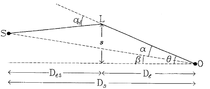
From the Figure follows the geometric relation

$$\theta D_{\rm S}=\beta D_{\rm S}+\alpha_{\rm d}D_{\rm LS}\,\,.$$ (2.45)

Substituting for $\alpha$ from (2.31), we rewrite it as

$$\beta=\theta-\frac{D_{\rm LS}}{D_{\rm L}D_{\rm S}}\frac{4GM}{c^{2}\theta}\equiv\theta-\frac{\theta_{\rm E}^{2}}{\theta}\,\,,$$ (2.46)

where

$$\theta_{\rm E}^{2}=\frac{4GMD_{\rm LS}}{c^{2}D_{\rm L}D_{\rm S}}\,\,.$$ (2.47)

Angle $\theta_{\rm E}$ denotes the angular radius, called the Einstein radius. It provides a natural angular scale to describe the lensing geometry. Sources which are closer than about $\theta_{E}$ to the optic axis are significantly magnified, whereas sources which are located well outside the Einstein ring are magnified very little. Besides, it is the radius of a tangential critical curve. In the given case of, the caustic is a point on tye optical axis. If a source is displaced slightly off the axis, two bright images are created on opposite sides of the lens centre, one just inside, and the other just outside the critical radius. The equation (2.46) has two real roots:

$$\theta_{1,2}=\frac{1}{2}\beta\pm\frac{1}{2}\sqrt{\beta^{2}+4\theta_{\rm E}^{2}}\,\,,$$ (2.48)

which correspond to two physical images of the source $S$. The angular separation between the images is

$$\Delta\theta=\theta_{1}-\theta_{2}=\sqrt{\beta^{2}+4\theta_{\rm E}^{2}}\geq 2\theta_{\rm E}\,\,.$$ (2.49)

The separation between the source and the deflector is related to the image position by

$$\theta_{1}+\theta_{2}=\beta\,\,.$$ (2.50)

Thus, the lens equation has two solutions of the opposite sign. The source has an image on each side of the lens, one inside Einstein radius, one outside. If the source is a disk of radius $\varphi_{\rm s}$, the images will represent ellipses, squeezed along the axis connecting them and stretched in perpendicular direction. For example, if $a,b$—semi-major axes, the area of ellipse is $\Omega=\pi ab$. The relations with the radius of the source we can write as

$$\frac{a}{\varphi_{\rm s}}=\frac{\theta_{1}}{\beta};\;\;\;\;\frac{b}{\varphi_{\rm s}}=\frac{d\theta_{1}}{d\beta}\,\,.$$ (2.51)

In the case of perfect alignment between source, lens and observer, ($\beta=0$), an observer will see a ring with radius $\theta_{\rm E}$ and thickness

$$\left.2\,\varphi_{\rm s}\,\frac{d\theta_{1}}{d\beta}\right|_{\beta\to\ 0}=2\varphi_{s}\left[\frac{1}{2}+\frac{1}{2}\,\frac{\beta}{\sqrt{\beta^{2}+4\,\theta_{\rm E}^{2}}}\right]=\frac{1}{2}\,2\varphi_{\rm s}=\varphi_{\rm s}\,\,,$$ (2.52)

equal to the source radius. The solid angle which it subtends on the sky is then $2\pi\theta_{\rm E}\varphi_{\rm s}$.

(ii) Magnifications

For a circular symmetric lens, the magnification factor $\mu$ (Eq. 2.41) is reduced to

$$\mu=\frac{\theta}{\beta}\frac{d\theta}{d\beta}\,\,.$$ (2.53)

For a point mass lens, which is a special case of a circular symmetric lens, we substitute for $\beta$ using the lens equation (2.46) to obtain the magnifications of the two images,

$$\mu_{\pm}=\left[1-\left(\frac{\theta}{\theta_{\pm}}\right)^{4}\right]^{-1}=\frac{u^{2}+2}{2u\sqrt{u^{2}+4}}\pm\frac{1}{2}\,\,,$$ (2.54)

where $u$ is the angular separation of the source in units of Eistein angle. The total magnification of the two images is

$$\mu=|\mu_{+}|+|\mu_{-}|=\frac{u^{2}+2}{u\sqrt{u^{2}+4}}\,\,.$$ (2.55)

$u=1$, or $\beta=\theta_{\rm E}$, is often taken to be a typical case that characterizes the efficiency of the lens. This corresponds to $\mu=1.34$ or $\Delta\mu=0.32$ in apparent magnitude. Point-like masses play an important role in the study of microlensing, which arises when the separation of the images is too small to be resolved and the lensing effect can only be observed through the lensing-induced time variability of the source.

Singular Isothermal Sphere

When we consider galaxies as lenses we need to allow for the distributed nature of the matter. The studies of the flat rotation curves of galaxies and the galaxy/gas distributions in clusters of galaxies suggest that the total matter profiles in these systems follow the singular isothermal sphere (SIS) model very well

$$\rho(r)=\frac{\sigma_{v}^{2}}{2\pi Gr^{2}}\,\,,$$ (2.56)

where $\sigma_{v}$ measures the line-of-sight velocity dispersion. In this model it is assumed that the mass components behave like particles of an ideal gas, confined by their combined spherically symmetric gravitational potential. It is assumed also that the gas is isothermal, so that $\sigma_{v}$ is constant across the galaxy $m\sigma_{v}^{2}=kT$. Upon projecting along the line-of-sight, we obtain the surface mass density

$$\Sigma(\xi)=\frac{\sigma_{v}^{2}}{2G\xi}\,\,,$$ (2.57)

where $\xi$ is the distance from the centre of the two-dimensional profile. Referring to Eq. 2.31, we find

$$\alpha_{\rm d}=4\pi\frac{\sigma_{v}^{2}}{c^{2}}\,\,,$$ (2.58)

which is independent of the impact parameter. The Einstein angle in this case is

$$\theta_{\rm E}=4\pi\frac{\sigma_{v}^{2}}{c^{2}}\frac{D_{\rm LS}}{D_{\rm S}}=\alpha_{\rm d}\frac{D_{\rm LS}}{D_{\rm S}}\,\,.$$ (2.59)

The solution to the lens equation $\beta=\theta-\theta_{\rm E}$ is

$$\theta_{\pm}=\theta_{\rm E}\pm\beta\;\;\;\;\mbox{for }\beta<\theta_{\rm E}\,\,.$$ (2.60)

Thus, the lens has two images on the oposite sides of the lens centre. For $\beta>\theta_{\rm E}$ only one image appears at $\theta=\theta_{+}=\beta+\theta_{\rm E}$. The image separation is just the diameter of the Einstein ring: $\Delta\theta=\theta_{+}+\theta_{-}\equiv 2\theta_{\rm E}$. Although the surface mass density is infinite at $\xi=0$, the behaviour of the model for larger values of $\xi$ seems to approximate the matter distribution of galaxies fairly well. Real galaxies, however, cannot follow the density law (2.56) due to an infinite density at the centre and an infinite mass. Other models exist and are frequently employed. For example, if the singularity is removed from the centre, the model is called a softened SIS—a SIS with a finite core radius $r_{\rm c}$ (ISC). In this case a lens is capable of producing either one, or three images. However, the usual absence of the third image implies that even if there is a core, it must be small, $\lower 2.58334pt\hbox{$\;\buildrel<\over{\sim}\;$}200$ parsecs [24].
The magnifications of the two images follow from Eq. 2.53 and are

$$\mu=\frac{|\theta|}{|\theta|-\theta_{\rm E}}\,\,,$$ (2.61)

the circle $|\theta|=\theta_{\rm E}$ is a tangential critical curve. Images are stretched in the tangential direction by a factor $|\mu|$, whereas the distortion factor in the radial direction is unity (see Section 2.3.4)

2.4 Astrophysical applications of gravitational lensing

Listing already existing and possible future astrophysical and cosmological applications of gravitational lensing is nearly an impossible task, so vast has become this field in the last years. Zwicky’s idea of the gravitational lensing as a cosmic telescope is proving itself with each observational discovery. We can see the magnified distorted images of galaxies which otherwise are far too dim to be observed, not to say, studied. Gravitational lensing effect allows us to test the General Relativity Theory, to probe the nature of the lensing object, the source and the intermediate space, and to test the large-scale structure of the universe. We will describe several interesting applications of gravitational lensing.

2.4.1 Determination of Hubble parameter and mass of the deflector

SSHubble parameter

One of the first applications of gravitational lensing, suggested by Refsdal [7], is the determination of the Hubble constant via the direct measurement of the time delay $\Delta t$ between the observed light curves of multiply imaged quasars. For axially symmetric lens this method can be described using the wavefront picture. Wavefront characterizes the locus of all points with equal light-time-travel from the source. Light rays in vacuum are perpendicular to the wavefronts, which are spherical close to the source. However, they become deformed by the gravitational field of deflector, may intersect themselves and cross the observer several times, producing multiple imaging. Every passage past the observer corresponds to the image of the source in the direction normal to the wavefront. The time delay for pair of images is the time between two crossings of the wavefront.

The wavefronts from a distant, doubly imaged quasar cross each other at the symmetry point. They represent the same light propagation time and for an observer, located at a distance $x$ from the symmetry axis, the time delay must be equal to the distance between the wavefronts at the observer divided by the velocity of light. The deflection law can be written as [7]

$$\alpha_{\rm d}\propto|\xi|^{\varepsilon-1}\,\,,$$ (2.62)

with $\varepsilon=0$ for a point mass lens. Using Hubble relation for small redshifts

$$cz=DH_{0}\,\,,$$ (2.63)

one obtains the expression for the Hubble parameter $H_{0}$ in terms of observable quantities

$$H_{0}\Delta t=\frac{1}{2}\frac{z_{\rm s}z_{\rm d}}{(z_{\rm s}-z_{\rm d})}\Delta\theta^{2}(2-\varepsilon)\,\,.$$ (2.64)

SSDetermination of mass

One more direct application of gravitational lensing is the determination of the mass of the deflector. The simplest situation here is when the lens is a spherically symmetric object and the source lies exactly behind the lens centre. The lens can then form an Einstein ring. In this case, the bending angle is

$$\alpha_{\rm d}(\theta)=\frac{4GM(<\theta)}{c^{2}D_{\rm L}\theta}\,\,,$$ (2.65)

and lensing equation with the source at the origin becomes

$$\theta=\alpha_{\rm d}(\theta)\frac{D_{\rm LS}}{D_{\rm S}}\,\,.$$ (2.66)

Combining these two equations we obtain

$$M(<\theta)=\pi(D_{\rm L}\theta)^{2}\Sigma_{\rm cr}\,\,.$$ (2.67)

The mass inside the Einstein ring can be determined, once its angular diameter and redshifts of the lens and the image are known. Even if the alignment of the source, deflector and the observer is not perfect, and the ring is not observed, this mass estimate may be very useful and rather accurate. For example, the mass inside the inner $0^{\prime\prime}.9$ of the lensing galaxy in the quadruple quasar QSO $2237+0305$ ("Einstein cross") has been determined with an accuracy of a few percent [14], with the largest uncertainty being due to the estimate of the Hubble constant. This method doesn’t depend on the nature or state of matter, but it measures only the projected mass and only in the inner part of the lensing galaxy.

Another method of determining the mass of the galaxy-deflector is from making use of the Eq. 2.64. From the observed image separation $\Delta\theta\simeq 2\theta_{\rm E}$ (Eq. 2.49) we find

$$2\theta_{\rm E} \simeq \theta_{1}+\theta_{2}$$

$$\theta_{\rm E}^{2} \simeq \frac{1}{4}\theta_{1}\theta_{2}$$

So that,

$$\left(\frac{\Delta\theta}{2}\right)^{2}\simeq\frac{4GMD_{\rm LS}}{c^{2}D_{\rm L}D_{\rm S}}\sim\frac{MH_{0}(z_{\rm s}-z_{\rm l})}{cz_{\rm s}z_{\rm l}}$$ (2.68)

Thus, the observed image separation $\Delta\theta\propto MH_{0}$, if the redshifts of the lens and the source are known. Using the relation between $\Delta t$ and $H_{0}$ (2.64) we obtain $M\propto\Delta t$. Thus, from the direct measurement of the $\Delta t$ one can determine the mass $M$ of the galaxy-lens located within an angular radius $\Delta\theta/2$.

Determination of the mass and mass distribution of the cluster of galaxies has become posible since the discovery of arcs and arclets. Arcs are the result of very strong distortion of background galaxies (when a part of an extended source covers different parts of the diamond-shaped caustic, associated with cluster of galaxies as a deflector). Assuming the cluster mass distribution to be axially-symmetric, we can have a rough mass estimate from (2.67), where $\theta$ now is the distance of the arc from the cluster centre, and $\Sigma_{\rm cr}$ can be determined, if the redshift of the arc can be determined. Also, since the arc roughly traces the Einstein radius, we can use the Eq. 2.47. This method loses accuracy if the cluster is highly asymmetric or has significant substructure (clumps of dark matter, for example). However, it is believed that the assumption, describing clusters as isothermal spheres with finite cores, works well [21].

Discovery of arclets (less elongated images of background galaxies than arcs) and weakly distorted images of background galaxies opened up the possibility of studying the mass distribution in the outer parts of the clusters. Shape of a galaxy image is affected by the tidal gravitational field along its corresponding light bundle. This distortion is small and since galaxies have intrinsically different shapes, the effect cannot be determined in the individual galaxy image. However, with the sky densely covered by randomly oriented faint galaxy images, a statistical study of the distortions of these far-away sources is possible. From the coherent alignment of images of an ensemble of galaxies one can draw the distortion pattern which traces the gravitational field of the foreground cluster. By reconstruction techniques one can measure the tidal field related to the gravitational potential of the cluster and obtain the surface mass density.

2.4.2 A candidate string-lensing field

One interesting aspect of the lensing phenomena is lensing by a straight cosmic string. Gravitational interaction of strings is characterized by the parameter $G\mu$, where $\mu$ is mass per unit length of the string $\mu\sim\eta^{2}$. Here $\eta$ is the energy scale of symmetry breaking $\sim 10^{16}$ GeV for grand unification scale. Thus,

$$G\mu\sim(\eta/m_{\rm pl})^{2}\,\,,$$ (2.69)

$m_{\rm pl}$—Planck mass $\sim 10^{19}$ GeV and $G=m_{\rm pl}^{-2}$. For grand unification strings $G\mu\sim 10^{-6}$ [25]. The metric around the straight string is flat, so it cannot be detected by gravitational interaction. However, the space around the string is actually a conical space, that can be made out of a Euclidean space by cutting out a wedge of angular size $\delta$ and by identifying the opposite sides of the wedge (Fig. 2.3).

Figure 2.3: The conical space around a straight string can be obtained from Eucledean space by cutting out the wedge of angular size $8\pi G\mu$ and identifying the exposed surfaces. Light rays emitted by quasar intersect behind the string and observer $O$ sees a double image of quasar $Q$. If $l$ and $d$ are the distances from the string to the quasar and to the observer, respectively, then the angular separation between the images is $\delta=8\pi G\mu l(d+l)^{-1}$.

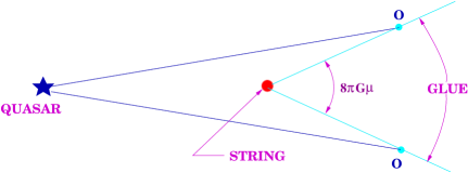
The deficit angle $\delta$ is $\delta=8\pi G\mu$. As seen from the Figure 2.3, the conical nature of space around the string can give rise to lensing phenomena. If there is an intervening string between us and background galaxy, such a string should produce an identical twin pair of images of the galaxy over a strip of space owing to an angle deficit $\delta$ around the string. The discovery of the field with a peculiar group of 4 “twin" galaxies was actually reported in a field near the quasar UM 679 [26].

These 4 pairs are remarkably twinlike with characteristic separations $\sim 2.4^{\prime\prime}$. The separation of the twins (and the width of the strip over which the splitting occurs) is determined by $\mu$ and a value $\sim 2.4^{\prime\prime}$ roughly corresponds to a string mass of $10^{-6}$ in dimensionless units. Further investigation of the candidate string-lensing field [27] revealed that in an area of $\pm 1^{\prime}$ around the original twins there are 7 twinlike galaxies, which satisfy the magnitude and color difference criteria for being lensing pairs. These twins vary wildly in magnitudes and colors but the distribution of separations is strongly peaked at $2^{\prime\prime}-2.5^{\prime\prime}$.

One more interesting phenomena can occur if the background source lies partially out of the wake since the galaxies are comparable in sizes with the lensing strip. Whereas a fully lensed galaxy should have the same color and spectrum in both images, in a partially lensed one the presence of strong color gradients, such as in a UV excess nucleus, can produce color differentiation between the images. Such an event was observed in the reported case. Here one member is bluer in continuum light, while the pair is identical in images of emission lines. Thefore, this object can be a partially lensed galaxy.

Strings can exist also in loops, though the exact metric of a long-lived loop string is unknown today. Its lensing properties in the linearised gravitational approximation were studied by Gott [28] and Wu [29]. It was shown that the loop can produce three images if the source is inside the loop; one is the original source seen through the loop, and two images on opposite sides from the light rays which passed outside the loop.

2.4.3 Detection of gravitational waves by lensing

Gravitational lenses can be used to detect gravitational waves, as a gravitational wave affects the travel-time of a light ray. In a gravitational lens, this effect produces time delays between the different images. Such "detectors" are 22 orders of magnitude larger than any of the existing or contemplated detectors, and they are sensitive to much lower frequences [30]. Time delay, produced by the wave, can be measured if the source (e.g., quasar) has variable brightness, thus producing images whith brightness variations correlated to a time-shift. For this purpose, the most useful systems would be those which are highly symmetric, so that the time delay due to the difference in the path length is small.

A gravitational wave affects the time delay because it perturbes the metric tensor, and therefore, modifies the path lenght of the two light rays. The metric is given by

$$g_{ab}=\eta_{ab}+h_{ab}$$ (2.70)

where $\eta_{ab}$ is the Minkowski metric, and $h_{ab}$ is a small perturbation. One can calculate the time delay by examining the influence of the metric perturbation on the equation of the null geodesic. The measured time delay in the lens system can then be used to put an upper limit on the amplitudes of stochastic background of the gravitational waves at low frequencies. Sensitivity of such a "detector" is greatest at wavelengths comparable to the overall size of the lens system. Allen [30] made such an estimation for the lens $0957+561$ for the frequency range $\omega>2\pi\times 10^{-18}$ Hz. The amplitude of the gravitational waves must be less than

$$h<2\times 10^{-5}\left[\frac{\omega}{2\times 10^{-17}}\right]\frac{sec}{radian}$$ (2.71)

or the expected time delay $\Delta t_{rms}$ would exceed the measured value of 420 days.

Though it may be difficult to separate the "intrinsic", geometrical time delay, from the delay caused by the gravitational wave, this idea may be still useful if the gravitational wave amplitude $h$ is larger than $\eta$, the angle between the images. The spatial motion of the geodesics that form the two images, induced by the gravitational wave, becomes significant. One effect of the gravitational perturbation is to change the angle between the images, usually by increasing it. The relative intensities of the two images also change.

2.4.4 Determination of the lens parameters from gravitationally lensed gamma-ray bursts

Recent results [31] from the Burst and Transient Source Experiment (BATSE) on the $Compton\ Gamma\ Ray\ Observatory$ show an isotropic distrubution of gamma-ray bursts across the sky and rule out a population of sources within the Galaxy. The most natural explanation is that the bursts have a cosmological origin. If $\gamma$-ray bursts occur at high redshifts, then some bursts are likely to undergo gravitational lensing by foreground matter. This would lead to the detection of multiple bursts with identical profiles but with different time delays and magnifications from a single event. Given a set of a multiple bursts (two or four), produced by a gravitational lens, what one one deduce about the nature of the lensing mass? Narayan and Wallington [32] showed that, if the lens is compact and pointlike, the quantity $(1+z_{\rm l})M$ can be determined directly from the observations without any information about the angular diameter distance to the lens or the source, and without knowledge of the source redshift. Here $M$ is mass of the lens and $z_{\rm l}$ is its redshift. What does a determination of $(1+z_{\rm l})M$ mean? First, it gives an upper bound on the lens mass

$$M_{\rm max}=(1+z_{\rm l})M=\left(\frac{c^{3}}{4G}\right)p_{1}\,\,,$$ (2.72)

where

$$p_{1}=\frac{(1+z_{\rm l})4GM}{c^{3}}\,\,.$$ (2.73)

This bound is independent of the size or geometry of the universe and of the redshift of the source or the lens. Second, if one can obtain an upper bound on $z_{\rm l}$, then one will also have a lower bound on $M$. Using the $V/V_{\rm max}$ data from BATSE, most cosmological models of gamma-ray bursts currently estimate the redshifts of the faintest observed sources to be $z_{\rm s}<1.5$. Accepting this estimate, we have $z_{\rm l}\leq 1.5$, and obtain the lower bound

$$M_{\rm min}=M_{\rm max}/(1+z_{\rm l,max})=M_{\rm max}/2.5\,\,.$$ (2.74)

The ability to bound the mass of the lens from both sides to within a factor of $\sim 2.5$ is an impressive accomplishment. For a point mass lens the measurable parameter $p_{1}$ has a magnitude given by

$$p_{1}=0.019(1+z_{\rm l})\left(\frac{M}{M_{\odot}}\right)\mbox{msec}\,\,,$$ (2.75)

which means that we can hope to detect point lenses with masses $>10^{2}M_{\odot}$. If a significant fraction of the mass of the universe is in the form of compact objects with masses of up to $\sim 10^{6}M_{\odot}$ in the dark halos of galaxies or in the intergalactic medium, then $\gamma$-ray bursts will reveal their presence through lensing and will provide accurate mass determinations. Moreover, once a sufficient number of lensed bursts has been detected, statistical techniques may be used to determine the fractional mass density $\Omega_{\rm lens}$ of the lenses [33].

If the lens is not pointlike but has an extended mass distribution, the observations can be used to obtain the velocity dispersion of the lens. If galaxy lenses are not singular, but have finite cores, then the image configuration will consist of three or five images. The extra burst will have the longest time delay and will generally be significantly weaker than the rest. The relative magnification of this burst will give useful information on the core radius of the lens.

2.4.5 Discovering planetary systems through gravitational microlensing

Traditional methods for the search of planetary systems involve either indirect observations (e.g. astrometry measurements) or direct infrared observations (search for dust lanes around the stars). A new method, based on the gravitational lensing of the bulge star by an intervening disk star was suggested in 1992 [34]. Planetary systems of galactic disk stars can be detected through microlensing of stars in the Galactic bulge. Planets in a solar-like system located half-way to the Galactic Centre should leave a noticeable signature on the light curve of a gravitationally lensed bulge star.

The gravitational lensing of distant sources by intervening individual compact masses, typically in the mass range $10^{6}\,M_{\odot}>M>10^{-4}\,M_{\odot}$, is called "microlensing". This term originates from the fact that the undetectable separation between images is of the order of microarcseconds for a solar mass located at a cosmological distance. For Galactic stars, however, the separation is of the order of a milliarcsecond. This angular separation is too small to observe. However, the resulting magnification can change the integrated light from the images for the time duration of the microlensing event. The brightness of the lensed star increases, peaks, and then decreases. The resulting light curve is smooth and completely described by three parameters: the temporal width, the maximum magnification and the time of maximum magnification. The duration of such an event is from several weeks to several months. It is symmetric in time about its maximum magnification and is achromatic, which allows one to distinguish it from variable stars.

If there is a planet around the lensing star, the light curve may be significantly altered. The planet of mass $m$ will typically affect the image magnification only for a fraction of $(m/M)^{1/2}$ of the duration of the entire event. With the typical stellar velocities ($\sim 200$ km/sec), this is a day or so for a Jupiter-mass planet. The observed light curve will look almost exactly like a light curve of an isolated star, except for a sharp spike during the fraction of time when a source moves inside a planetary Einstein radius. The planet affects appreciably the microlensed image only if the planet and the unperturbed image are separated by a distance of the order of the planet’s own Einstein radius, $(4GMD_{\rm eff}/c^{2})^{1/2}$, where $D_{\rm eff}=D_{\rm L}D_{\rm S}/D_{\rm LS}$.

The probability of detecting such events in the total number of microlensing events can be estimated. If a solar-like planetary system lay at a random position along the line of sight to the Galactic bulge, and if the bulge source came within one Einstein radius of the central star of this system, then the system could be detected $\sim 20$% of the time (assuming minimum detectable perturbation $\delta_{min}=5$%). The largest contributor will be a Jupiter-like planet, $\sim 17$%, Saturn-like will give $\sim 3$%, and all the other planets $\ll 1$%.

From the light curve the ratio of planetary to stellar mass, $\epsilon=m/M$, can be determined. If the lensing star is a G dwarf or earlier, its spectrum can be taken. From the spectral type and the luminosity one may determine the mass and distance and, thereby, infer the mass of the planet and its projected distance from the star. The typical planetary signal lasts for a day or less. Thus, to detect a Jupiter-mass planet, observations should be taken every 4 hours, detection of a Neptune-mass planet will require hourly observations.

2.4.6 Light deflection in strong gravitational fields

Up to now we were considering weak gravitational fields, where the essential assumption for lensing formalism is that the bending angles of light rays are very small. All tests of GTR within the Solar System, including the bending and delay of light rays passing the Sun, have examined the gravitational interaction only in connection with weakly self-gravitating objects (for example, the Sun has a surface gravitational potential $GM/c^{2}R\approx 2\times 10^{-6}$). The measured relativistic effects are but small perturbations to Newtonian mechanics and these tests say nothing about the strong field situation. There are, however, astrophysical systems where gravitational fields are strong and light bending leads to new interesting effects. Observing such systems and measurement of their parameters can yield tests of GTR to a greater precision.

GL Effects in Accreting Systems

SSRelativistic "looks" of a neutron star

General relativistic effects are quite substantial for neutron stars (NS) of radii smaller than about $2r_{\rm S}$, where $r_{\rm S}=2GM_{\rm NS}/c^{2}$ is the Schwarzschild radius of NS. One expects these effects to play a major role in the interpretation of the spectrum and light curves of such stars. The characteristic quantity here is the ratio $\rho=r_{*}/r_{\rm S}$, where $r_{*}$ is NS’s radius. For stars with $\rho\leq 2$ radiation emitted deep inside the strong gravitational field of such a star will be significantly modified as seen by the distant observer. Light ray, emitted on or near the surface will be redshifted and may be deflected by more than $45^{0}$ [35].

It was shown that rays reach the observer with larger impact parameters than they would in flat space and, in addition, photons from the "back" half of the star can reach the observer. As a result, the part of the star which would be visible in flat space now appears larger and we may see parts of the star which would otherwise be hidden from view. While in flat spacetime exactly half of the surface of the star is visible, for $\rho>1.7$ the whole star becomes visible, the point at $180^{0}$ appears as the circular boundary of the disk.

For the NS with emission from polar regions the visibility of the hot spots is markedly different from the flat space case. Ref. [35] shows the simulated picture of a pair of antipodal hot spots at 12 different phases of rotation with the angle between rotation axis and a hot spot to be $45^{\circ}$.

Light curves from relativistic neutron stars

Pechenick et al [36] have investigated the influence of GL effects on the beaming of radiation from a hot spot on the surface of a slowly rotating star in the limit where Schwarzschild metric is applicable. It was demonstrated that the deflection of light in the vicinity of a NS produces large deviations of model light curves from those expected in the absence of gravitational effects. For thermal emission, gravity tends to flatten the light curve for the NS with $\rho\geq 2$, giving very little observed variation for nominal pulsar values. For NS with $\rho\leq 2$ a new feature appears in the form of a spike at $\theta=0^{\circ}$, whose width is about the angular diameter of a polar cap and whose relative height increases with decreasing of a polar cap radius. For the most relativistic case this feature represents a jump of $1.2\,mag$ over the essentially flat continuum. The sharp peak is actually due to the gravitational lensing effect of the star on the cap at $\theta=180^{\circ}$ to the line of sight. It arises from photons emitted near the tangential plane and bent through large angles (up to $227^{\circ}$). The region near $\theta=180^{\circ}$ appears as a ring whose apparent brightness exceeds that of a comparable region at $\theta=0^{\circ}$. Thus, gravity alone is capable of producing strongly beamed radiation even for isotropically radiating polar caps.

These results are applicable to the structure of $X$-ray pulsars in binary systems where accretion is assumed to give rise to hot polar regions. That the $X$-ray light curve arises simply from rotational eclipsing of these caps seems unlikely. One interesting possibility is that emission originates above the NS surface. It was demonstrated that for the NS with $\rho=2.5$ any emitting region higher than $0.19R_{\rm NS}$, regardless of shape and size, will always be in view. For a typical NS no point that is more than 2 or 3 km above the surface is ever out of sight. For accreting pulsars it would be relevant for the case when the infalling matter decelerates at some distance above the surface due to shocks or radiation pressure. In this case, one has an accretion "column" rather than a polar cap or hot spot. In the general relativistic treatment of the emission from the column, there appear two new qualitatively different effects [37]. First, the frequency redshift is different for radiation arising from different heights. Second, the star and the accretion column will both produce some shadowing of the light rays. This effect depends on the emission height and on the direction of observation. In general, one sees that the column beam is strongly backwardly bent for the most relativistic cases.

Emission from accretion disk

The spectrum of X-rays produced by an accretion disk around a black hole is influenced markedly by GL effects [38]. Due to the forward "peaking" of the emitted radiation by the rapidly moving gas in the inner disk and to the gravitational focusing, the radiation is concentrated toward the equatorial plane. The concentration toward the plane from the inner disk is more severe for large values of $a/M$, where $a$ is angular momentum per unit mass and $M$ is mass of the black hole. As the disk thickens in its outer regions, a distant observer directly in equatorial plane is in a shadow and in Newtonian case (disk accretion model neglecting the relativistic effects) receives no radiation. In actuality, he sees some blueshifted radiation from every radius outside the radius of marginal stability $r_{\rm ms}$ (radius at which gas begins to plunge into the hole). Radiation seen by other observers is less blueshifted, and that seen by the axial observer is always redshifted. For a Schwarzschild black hole, the effects of redshift and focusing are minor, since a disk around such black hole has a large inner radius ($r_{\rm ms}=6M)$. Only the equatorial observer sees a spectrum different from Newtonian spectrum (since this observer sees only focused radiation he always sees a spectrum dominated by high-energy radiation from the inner disk). For Kerr black hole with $a\leq 0.9M$ redshift and focusing effects on the observed spectrum are striking. Even though all observers receive practically the same integrated flux, the average photon energy differs by approximately an order of magnitude between the equatorial and axial observer. The axial observer sees radiation from the cold, outer regions of the disk primarily; radiation from the inner regions is redshifted and defocused. Consequently, he sees a spectrum, attenuated at high energies in comparison to the Newtonian spectrum. The equatorial observer sees radiation from the hot, inner region to be blueshifted and strongly focused, consequently, spectrum is enhanced at high energies, compared with the Newtonian. If emission is not isotropic, for the axial observer $n_{\rm e}\approx 0$ ($n_{\rm e}$—the angle of the emitted radiation with the surface normal) for radiation from large radii. This angle increases as $r_{\rm e}$ decreases. For other observers, the emission angle decreases as $r_{\rm e}$ increases, reaching a minimum for $r_{\rm e}=3-4M$. The radius for min $n_{\rm e}$ is smallest for the equatorial observer. Thus, radiation reaching the observer from very small radii has large emission angles. Near the horizon radiation must be emitted parallel to the disk surface to escape being trapped by the disk or the hole.

GL Effects in Compact Binaries

Compact binaries present a unique laboratory for testing GR in the strong-field limit. This has become possible due to increasing discoveries of binaries, where one compact object is a neutron star (pulsar, beaming at us) and the other is a white dwarf (WD) (for example, 1855+09), a neutron star (NS) (for example, 1913+16 system) or a black hole (BH) (for example, a binary PSR B0042-73 in SMC is argued to have a massive $10--30\,M_{\odot}$ BH companion [39]).

To date, there exists one test of relativistic gravity [40], the $\dot{\omega}-\gamma-\dot{P_{b}}$ test. It is obtained by combining the five timing parameters of the binary: eccentricity—$e$, orbital period—$P$ and three "post-keplerian" (PK) ones: advance of periastron $\dot{\omega}$, time dilation and gravitational shift parameter $\gamma$ and the orbital period decay $\dot{P}$. All these are linked by the theory-dependent constraint, which can be defined as $\dot{P}/f^{\rm theory}(e,\,P,\,\gamma,\,\dot{\omega})=1$. For PSR 1913+16 Damour [40] finds

$$\frac{\dot{P^{obs}}}{f^{\rm GR}(e^{obs},\,P^{obs},\,\gamma^{obs},\,\dot{\omega^{obs}})}=0.995\pm 0.021$$ (2.76)

By contrast, in other theories of gravity the influence of strong-field effects on the function $f^{theory}(e,\,P,\,\gamma,\,\dot{\omega})$ is enormous and it changes drastically both in sign and in magnitude [40]. Therefore, this result constitutes good (better than $0.5\%$ accuracy [41]) confirmation of GR and, above all, a very selective confirmation of the ability of GR to describe the strong (and$/$or rapidly varying) gravitational fields. The $\dot{\omega}-\gamma-\dot{P_{b}}$ test is a mixed test, which combines strong-field effects (related to $\dot{\omega}$ and $\gamma$) with radiative effects (related to $\dot{P}$). Thus, one cannot logically conclude, when it is satisfied, that both the specific strong-field and radiative predictions of GR have been independently confirmed [42]. In the case of a binary’s orbit inclination to the sky plane approaching $90^{\circ}$ the pulsar’s two more PK parameters, characterizing the range $r\equiv Gm_{c}/c^{3}$ and the shape $s\equiv\sin{i}$ of the Shapiro time delay, may be measured. This has already allowed the determination of the neutron star mass with a precision better than $18\%$ (B1855+09 [43]).

Self-lensing by binaries

Eclipsing binaries present a remarkable situation where, if the orbital plane inclination to the plane of the sky is close to $90^{\circ}$, the gravitational amplification of the companion by the compact object is possible. The observable effect here is periodic brightness enhancement which would depend on the geometry of the system. Schneider [44] gives for the binary pulsar PSR $1957+20$ the periodic brightness amplification between $10^{-4}$ and $10^{-2}$, with a probability that amplification really exists at about $10\%$, if an adopted radius of optical companion is $R_{c}=0.1R_{\odot}$. For an impact parameter $b=0$, the duration of amplification is of $\,T_{\rm A}\approx 400$ sec. Though the variability in brightness of an optical companion was observed in the case of PSR1957+20, Schneider warns that it is still difficult to make the presently predicted amplification observable. The star can have intrinsic variability due to the geometry of the "evaporation" mechanism driven by the pulsar. Gould [45] suggested monitoring millisecond binaries to search for lensing events. He showed that self-lensing in binary pulsars could be used to probe the structure of the emitting region of pulsars, in particular, to check whether the emission originates from the light cylinder or from a smaller locus. For pulsars of period $P$, the light cylinder has a radius $Pc/2\pi\approx 10^{8}\,[P/(20\,ms)]\,cm$. If the lensing magnification curve follows the classic form for a point source, this would show that the source is small on scales of the Einstein ring, $R_{\rm E}\approx 3\times 10^{8}\,(a/10^{11})^{1/2}$ cm.

Deflection of the light beam by companion

If the inclination of the sky plane of the orbit of binary pulsar $i$ is close to $90^{\circ}$, the pulsar beam during a fraction of the orbital revolution will be gravitationally deviated by the companion and this effect will manifest itself in the timing formulae. Bending of the pulsar beam by a companion can lead to the deviation of the apparent position, to brightness amplification of the source and to time delays. As in the Shapiro effect, the deflection of pulsar’s beam shows in the timing as a rapid, sharp growth of the magnitude of the post-fit residuals of times-of-arrival (TOAs) on a short time interval during the superior conjunction of the pulsar and its companion. This effect is superimposed on the Shapiro effect [46].

Pulsar’s TOAs are determined by measuring the phase offset between each observed profile and a long-term average one. In addition, a set of post-fit residuals are determined—the differences between measured TOAs and those calculated using the classical spin-down model of pulsar rotation. When many TOAs are available, spaced over months or years, it generally follows that, at least the pulsar’s celestial coordinates, spin parameters and Keplerian orbital elements will be measurable with high precision. The binary systems most likely to yield measurable PK parameters are those with large masses, high eccentricities and astrophysically "clean", so that orbits are mostly dominated by gravitational interactions between two compact masses. Apart from mass determination, measurement of the light deviation effect in near edge-on compact binaries would help to get further constraints on the position of the pulsar’s spin. In this effect the shape of TOAs residuals strongly depends on the spatial orientation of the pulsar’s rotational axis [46].

Epstein [47] was, perhaps, the first who paid attention to the phenomenon of pulsar beam deviation in the gravitational field of it’s companion in the case of $\cos i\leq 10^{-3}$. To be detected, the PSR beam must, after each revolution, point in the direction defined by the null geodesic connecting the orbital location of the pulsar to the observer. Due to the light bending produced by the gravitational field, this direction depends on the orbital phase. The result of this gravitational shift is a delay due to the excess angle swept out by the pulsar in each spin period. The influence of two relativistic effects (Shapiro and gravitational shift) should be compared with the special relativistic effect—abberation, which also causes shifts of the pulsar beam and delays. The discussion on the importance of the different delays appears in [48]. Author discussed the importance of the different delays which must be included in the timing formulae of binary system with orbit inclination close to $90^{\circ}$ to the line of sight. He studies the gravitational shift delay for compact binaries at orbital phases close to superior conjunction. For PSR 0655+64, Schneider derives delays of $1-10\mu$s (due to the gravitational shift effect) during a small fraction of the orbital period. Observation of this delay in a binary system must be considered as evidence that pulsars are indeed rotating beacons, instead of stars with periodic isotropic flares [49]. All derivations are done in standard Schwarzschild formalism, neglecting the changes imposed by the mass of the pulsar in the system, which bears some justification. When the pulsar mass is assumed to be negligible, there exists only one geodesic, radial, joining the centres of the two stars. More than one such path would imply that a photon emitted radially from the centre of the companion star can aquire a transverse motion, which is not possible in the Schwarzschild solution. However, once the mass of the pulsar is "switched on", there exists a family of geodesics between the two stars, all of which have geometric path lengths greater or equal to the initial radial one. The addition of the pulsar mass must increase all geodesic path lengths and those passing near to both stars the most. Thus, it appears that the corrections due to the pulsar mass can only increase the magnitude of the predicted effects [50].

Doroshenko and Kopeikin [46] reduced the favourable inclination angle to cos$i\leq 0.003$ and showed that this estimate becomes less restrictive as the pulsar’s spin axis approaches the line of sight. For the first time they showed the time behaviour of the residuals of the TOA in the vicinity to the moment of superior conjunction of the pulsar and its companion. Their numerical estimates showed that beam deviation effect is too small to be detected in the presently the best available example of PSR B1855+09 with cos$i=0.04$.

Chapter 3 Gravitational Lensing as a Tool in Search of Natural Wormholes and Negative Matter in the Universe.

3.1 Introduction

Energy conditions and their violations

The energy conditions (EC) of classical GR for a case of FRW spacetime are a set of simple constraints on various linear combinations of the energy density and pressure. They are the null (NEC), the weak (WEC), the strong (SEC), and the dominant (DEC) energy conditions. For a FRW spacetime and a diagonal stress-energy tensor $T_{\mu\nu}=(\rho,-p,-p,-p)$ with $\rho$ the energy density and $p$ the pressure of the fluid, they read:

NEC $$\iff \quad(\rho+p\geq 0),$$

WEC $$\iff \quad(\rho\geq 0)\hbox{ and }(\rho+p\geq 0),$$

SEC $$\iff \quad(\rho+3p\geq 0)\hbox{ and }(\rho+p\geq 0),$$

DEC $$\iff \quad(\rho\geq 0)\hbox{ and }(\rho\pm p\geq 0).$$ (3.1)

The EC are, then, just simple constraints on various linear combinations of the energy density and the pressure of the matter generating the spacetime curvature. Since normal matter has both positive energy density and positive pressure, it automatically satisfies the null, weak and strong energy conditions. If we impose the condition that speed of sound in normal matter is less than the speed of light, we would have in addition $\,\partial\rho/\partial p<1$. Assuming there is no cosmological constant, integrating this gives $p<\rho$, so that dominant energy condition is satisfied as well. Roughly speaking, the violation of the DEC is usually associated with either a large and negative cosmological constant, or with superluminal acoustic modes. Quite recently, it was shown [51] that the presently favoured value of Hubble parameter [$H_{0}=(65,85)$] implies that SEC must be violated somehere between the epoch of galaxy formation and the present. Since normal matter satisfies SEC, this would require the introduction of “abnormal matter" (we would need large quantities of abnormal matter, sufficient to overwhelm the gravitational effects of normal matter). Violating the SEC is usually associated with a positive cosmological constant or cosmological inflationary epoch.

In the 60’s and 70’s these energy coonditions were widely used as key foundations for a number of important theorems. For example, for “the positive mass theorem" (which states that objects made of the matter that satisfies the DEC can never antigravitate), for a variety of theorems that predict the creation of singularities in stellar collapse and in cosmological scenarios. The discovery of Hawking that nonrotating black holes can evaporate and, correspondingly, their surface area can shrink (in direct violation of the area increase theorem—“second law of black hole mechanics", based on the SEC) forced physicists to face the fact that though in classical physics the EC are perfectly reasonable assumptions, quantum fields can violate them. Many physical systems, both theoretical and experimental, are known to violate one or more EC. Perhaps, the most quoted is the Casimir effect (for more information on this and other examples, see [12]). Typically, observed violations are of quantum nature and are of the order of ${\raise-0.15pt\hbox{$\mkern-0.5mu\barbar$}\mkern-8.5muh}$. It is currently far from clear whether there could be macroscopic violations of EC. If they do exist, macroscopic negative masses could be part of the ontology of the universe.

Negative Masses

The violations of the EC, in particular the weak one, would admit the existence of negative mass. The possible existence of negative gravitational masses has been investigated since the end of the nineteenth century [52]. From a Newtonian point of view, we can differentiate four possible situations [53]: (i) both inertial and gravitational masses are positive, (ii) inertial mass is positive and gravitational mass is negative, (iii) inertial mass is negative and the gravitational mass is positive, and (iv) both inertial and gravitational masses are negative. Most of the Nineteenth Century literature on negative masses is devoted to case (ii). From a relativistic point of view, however, the situation is quite different: the Equivalence Principle (EP) requires that gravitational and inertial masses cannot be considered distinct any longer. Test particles move along geodesic lines in accordance with the initial conditions, independently of the fact that their energy density is positive or negative. Negative energy densities or negative masses exert a repulsive force not only for ordinary matter, but for exotic matter as well. This might conceivably pose a stability problem for large amounts of exotic material, requiring large values of tension in order to keep an equilibrium configuration [54]. In more complicated astrophysical systems stability could be achieved through electromagnetic forces.

Wormholes

Of all the systems which would require violations of the EC in order to exist, wormholes are the most intriguing. The salient feature of these objects is that an embedding of one of their spacelike sections in Euclidean space displays two asymptotically flat regions joined by a throat. Wormholes basically represent bridges between otherwise separated regions of the spacetime (Fig. 3.1) and need a special kind of matter in order to exist. This matter, known as exotic, violates the EC.

Figure 3.1: Left: Embedding diagramme for a wormhole. Two mouths, joined by a tunnel, can connect regions otherwise separated or disconnected (here the normal space should fold as a sheet of paper, whereas the wormhole would be a tunnel from one side of the sheet to the other). Right: Embedding diagram for a black hole. The singularity here is represented as a pinch off of the wormhole tunnel.

Wormhole solutions to the Einstein field equations have been extensively studied in the last decade (for the detailed description of the wormhole solution see Appendix A). A simple search in PRD online resources yields 57 papers in the last three years including the word "wormhole" in its full record. Msot of these are works deal with different trials to find analytical solutions representing Lorentzian wormholes in space-time. There are known wormhole solutions representing rotating structures, charged, uncharged, static, evolving wormholes, wormholes within alternative gravity theories, etc. But, clearly, this is only one aspect of the problem. Once one has an analytical solution, it is not at all clear that the physical constructs it represents can, or do, indeed, exist. This second aspect of the problem is not commonly treated in the literature: very little work has been done to develope astrophysical, or other kind of tests, to see whether wormholes really are part of the ontology of the universe (see [12, 55] and references cited therein.

Can a wormhole have total negative mass?

Since wormholes have to violate the null energy condition in order to exist, the hypothesis underlying the positive mass theorem no longer applies. There is nothing in principle that can then prevent the occurrence of a negative total mass. In other words, we need to have some negative mass near the throat to keep the wormholes open [56]. Examples of wormhole solutions, both with positive and negative mass, followed the pioneering work by Morris and Thorne [54] (see [12] for a review). Visser, for instance, suggested a particular class of solutions, lacking spherical symmetry, configurations in which there is a flat-space wormhole, framed by struts of an exotic material [57]. These kinds of wormholes and many others, including the simplest one known as absurdly benign wormhole [54], would have a negative mass density. Typically near the throat the following relationship would hold:

$${\rm mass\;at\;throat}=-\frac{{\rm radius}\cdot c^{2}}{G}\,\,.$$ (3.2)

For a radius equal to 1 meter the mass of the mouth will be equal to $-1$ Jupiter mass. The total mass seen at infinity will depend on the details of the model, such as the neighboring matter, and can be positive, negative or zero according to the specific case. Whether or not mass separation is possible is not clear yet.

Some speculations have been made about how inflation can be responsible to enlarge a microscopic wormhole—believed to exist in the Planck foam—out to macroscopic dimensions [58]. This mechanism could result in a population of natural wormholes.

Large-scale violations and observational strategy

The result of the already mentioned work [51] on the violation of SEC in the recent epoch could imply the existence of a massive scalar field or a positive cosmological constant. These are favoured by current observations. Even if the global energy density of the universe is WEC-respecting, it is still not clear whether there exist spacetime domains where large-scale violations of the EC occur, allowing the formation of physical systems with an energy density equivalent to a total negative mass of the size of a galaxy or even a cluster of galaxies.

Fifteen years after the seminal paper by Morris and Thorne [54], we face the following situation: there is no observational evidence supporting the existence of natural wormholes or serious theoretical reasons for their impossibility. Blackholes shared such a status during years until the discovery of galactic x-ray sources and quasars in the 1960s. Clearly, we have no better way than devising observational tests for deciding the existence of negative masses. For instance, if natural wormholes with negative masses or spacetime domains having large-scale violations of the EC actually exist in the universe (e.g. if the original topology after the Big-Bang was multiply connected), then there could be some observable electromagnetic signatures that might lead to their identification. The approach of the present work points out in this direction: we do not know whether there exist an astrophysical population of objects with negative mass, but if they indeed exit, then we provide specific observational signatures that we can expect.

Previous Studies on Lensing by Negative Masses

The idea that wormholes can act as gravitational lenses and induce a microlensing signature on a background source was first suggested by Kim and Sung [59]. Unfortunately, their geometry was that of a perfect alignment of a source, both wormhole’s mouths and an observer, which is quite unlikely. They also considered both mouths to be of positive mass. Cramer et al. [60] carried out more detailed analysis of negative mass wormholes and considered the effect they can produce on background point sources at non-cosmological distances. The generalization to a cosmological scenario was carried out by Torres et al. [61], although lensing of point sources was still used. As far as we are aware, the first and only bound on the possible existence of negative masses, imposed using astrophysical databases, was given by Torres et al. [61]. Recently, Anchordoqui et al. [62] searched in existent gamma-ray bursts databases for signatures of wormhole microlensing. Although they detected some interesting candidates, no conclusive results could be obtained. Peculiarly asymmetric gamma-ray bursts [63], although highly uncommon, might be probably explained by more conventional hypothesis, like precessing fireballs (see, for instance, Ref. [64]).

In the following sections we describe microlensing by natural wormholes of stellar and sub-stellar masses. We provide an in-depth study of the theoretical peculiarities that arise in negative mass microlensing, both for a point mass lens and source, and for extended source situations. We present negative mass microlensing simulations, showing the resulting shapes of the images, the intensity profiles, the time gain function, the radial and tangential magnifications, and other features. Our work extends and deepens previous papers in several ways, and gives a method of analyzing observational predictions quantitatively.

In the last section of this chapter we present the results of a set of simulations showing macrolensing effects we could observe if such a large amount of negative energy density existed in our universe.

3.2 Negative mass lensing formalism and basic equations for a point lens

In this chapter we consider lensing only by a point negative mass lens, and thus we can use all the assumptions concurrent with the treatment of the Schwarzschild lens (see Section 2.3.5). The image coordinates can be written as $(\theta_{1},\theta_{2}$) and those of the source as $(\beta_{1},\beta_{2})$.

3.2.1 Effective refractive index of the gravitational field of a negative mass and the deflection angle

The ‘Newtonian’ potential of a negative point mass lens is given by

$$\Phi(\xi,z)=\frac{G|M|}{(b^{2}+z^{2})^{1/2}}\,\,,$$ (3.3)

where $b$ is the impact parameter of the unperturbed light ray and $z$ is the distance along the unperturbed light ray from the point of closest approach. We have used the term Newtonian in quotation marks since it is, in principle, different from the usual one. Here the potential is positively defined and approaches zero at infinity [12]. In view of the assumptions stated above, we can describe light propagation close to the lens in a locally Minkowskian spacetime perturbed by the positive gravitational potential of the lens to first post-Newtonian order. In this weak field limit, we describe the metric of the negative mass body in orthonormal coordinates $x^{0}=ct$, ${\bf x}=(x^{i})$ by

$$ds^{2}\approx\left(1+\frac{2\Phi}{c^{2}}\right)c^{2}dt^{2}-\left(1-\frac{2\Phi}{c^{2}}\right)dl^{2},$$ (3.4)

where $dl=|{\bf x}|$ denotes the Euclidean arc length. The effect of the space-time curvature on the propagation of light can be expressed in terms of an effective index of refraction $n_{\rm eff}$ given by

$$n_{\rm eff}=1-\frac{2}{c^{2}}\Phi\,.$$ (3.5)

Thus, the effective speed of light in the field of a negative mass is

$$v_{\rm eff}=c/n_{\rm eff}\approx c+\frac{2}{c}\Phi\,.$$ (3.6)

Because of the increase in the effective speed of light in the gravitational field of a negative mass, light rays would arrive faster than those following a similar path in vacuum. This leads to a very interesting effect when compared with the propagation of a light signal in the gravitational field of a positive mass. In that case, light rays are delayed relative to propagation in vacuum—the well known Shapiro time delay. In the case of a negative mass lensing, this effect is replaced by a new one, which we shall call time gain. We will describe this effect in more detail in the following subsections. Defining the deflection angle as the differenceof the initial and final ray direction

$$\boldsymbol{\alpha}:=\hat{\bf e}_{\rm in}-\hat{\bf e}_{\rm out},$$ (3.7)

where $\hat{\bf e}:=d{\bf x}/dl$ is the unit tangent vector of a ray ${\bf x}(l)$, we obtain the deflection angle as the integral along the light path of the gradient of the gravitational potential

$$\boldsymbol{\alpha}=\frac{2}{c^{2}}\int\boldsymbol{\nabla}_{\bot}\Phi dl\,\,,$$ (3.8)

where $\boldsymbol{\nabla}_{\bot}\Phi$ denotes the projection of $\boldsymbol{\nabla}\Phi$ onto the plane orthogonal to the direction $\hat{\bf e}$ of the ray. We find

$$\boldsymbol{\nabla}_{\bot}\Phi(b,z)=-\frac{G|M|{\bf b}}{(b^{2}+z^{2})^{3/2}}\,.$$ (3.9)

Eq. 3.8 then yields the deflection angle

$$\boldsymbol{\alpha}=-\frac{4G|M|{\bf b}}{c^{2}b^{2}}\,\,.$$ (3.10)

It is interesting to point out that in the case of the negative mass lensing, the term ‘deflection’ has its rightful meaning—the light is deflected away from the mass, unlike in the positive mass lensing, where it is bent towards the mass.

3.2.2 Lensing geometry and lens equation

Figure 3.2: Lensing geometry of a negative mass. $O$ is the observer, $S$ is the source, $W$ is the negative mass lens, $I_{1}$ is one of the images. $\beta$ is the angle between the source and the lens—position of the source, $\theta$ is the angle between the source and the image—position of the image, and $\alpha$ is the deflection angle. $b$ is the impact parameter and $D_{l}$, $D_{s}$ and $D_{ls}$ are angular diameter distances. Other quantities are auxiliary.

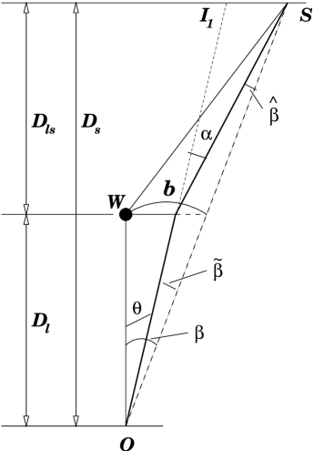
In Fig. 3.2 we present the lensing geometry for a point-like negative mass. From this figure and the definition of the deflection angle (Eq. 3.10), we can obtain the relation between the positions of the source and the image. We only need to relate the radial distance of the source and the image from the center, since due to circular symmetry, the azimuthal angle $\phi$ is not affected by lensing. This gives

$$(\boldsymbol{\beta}-\boldsymbol{\theta})D_{\rm s}=-\boldsymbol{\alpha}D_{\rm ls}$$ (3.11)

or

$$\boldsymbol{\beta}=\boldsymbol{\theta}-\frac{D_{\rm{ls}}}{D_{\rm s}}\boldsymbol{\alpha}\,\,.$$ (3.12)

With the deflection angle (Eq. 3.10), we can write the lens equation as

$$\beta=\theta+\frac{4G|M|}{c^{2}\xi}\frac{D_{ls}}{D_{s}}=\theta+\frac{4G|M|}{c^{2}}\frac{D_{ls}}{D_{s}D_{l}}\frac{1}{\theta}\,\,.$$ (3.13)

3.2.3 Einstein radius and the formation of images

A natural angular scale in this problem is given by the quantity

$$\theta^{2}_{\rm E}=\frac{4G|M|}{c^{2}}\frac{D_{\rm ls}}{D_{\rm s}D_{\rm l}}\,\,,$$ (3.14)

which is called the Einstein angle. In the case of a positive point mass lens, this corresponds to the angle at which the Einstein ring is formed when the source, lens and observer are perfectly aligned. As we will see later in this section, this does not happen if the mass of the lens is negative. There are other differences as well. A typical angular separation of images is of order $2\,\theta_{\rm E}$ for a positive mass lens. Sources which are closer than about $\theta_{\rm E}$ to the optical axis are significantly magnified, whereas sources which are located well outside the Einstein ring are magnified very little. All this is different with a negative mass lens, but nonetheless, the Einstein angle remains a useful scale for the description of the various regimes in the present case and, therefore, we shall use the same nomenclature for its definition.

The Einstein angle corresponds to the Einstein radius in the linear scale (in the lens plane):

$$R_{\rm E}=\theta_{\rm E}D_{\rm l}=\sqrt{\frac{4GM}{c^{2}}\frac{D_{\rm ls}D_{\rm l}}{D_{\rm s}}}\,\,.$$ (3.15)

In terms of Einstein angle the lens equation takes the form

$$\beta=\theta+\frac{\theta_{\rm E}^{2}}{\theta}\,\,,$$ (3.16)

which can be solved to obtain two solutions for the image position $\theta$:

$$\theta_{1,2}=\frac{1}{2}\left(\beta\pm\sqrt{\beta^{2}-4\theta_{\rm E}^{2}}\right).$$ (3.17)

Unlike in the lensing due to positive masses, we find that there are three distinct regimes here and, thus, can classify the lensing phenomenon as follows:

1. $\beta<2\theta_{\rm E}$  There is no real solution for the lens equation. It means that there are no images when the source is inside twice the Einstein angle.

2. $\beta>2\theta_{\rm E}$  There are two solutions, corresponding to two images both on the same side of the lens and between the source and the lens. One is always inside the Einstein angle, the other is always outside it.

3. $\beta=2\,\theta_{\rm E}$  This is a degenerate case, $\theta_{1,2}=\theta_{\rm E}$; two images merge at the Einstein angular radius, forming the radial arc (see Section 3.2.5).

Figure 3.3: Formation of images by a point negative mass lens. S is the source, $\bf I_{1}$ is the outer image and $\bf I_{2}$ is the inner image. Lens is in the centre, $\theta_{\rm E}$ is the angular scale of the lensing. This Figure shows schamaticall the radial distortion of images in the case of a negative mass lens.

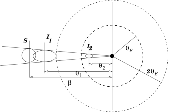
We also obtain two important scales, one is the Einstein angle ($\theta_{\rm E}$)—the angular radius of the radial critical curve, the other is twice the Einstein angle ($2\,\theta_{\rm E}$)—the angular radius of the caustic. Thus, we have two images, one is always inside the $\theta_{\rm E}$, one is always outside; and as a source approaches the caustic ($2\,\theta_{\rm E}$) from the positive side, the two images come closer and closer together, and nearer to critical curve, thereby brightening. When the source crosses the caustic, the two images merge on the critical curve ($\theta_{\rm E}$) and disappear. In Fig. 3.3 we show schematically the formation and positions of images for the negative mass lensing.

3.2.4 Time gain and time-offset function

Following [20], we define a scalar potential, $\psi(\boldsymbol{\theta})$, which is the appropriately scaled projected Newtonian potential of the lens,

$$\psi(\boldsymbol{\theta})=\frac{D_{\rm ls}}{D_{\rm l}D_{\rm s}}\frac{2}{c^{2}}\int{\Phi(D_{\rm l}\boldsymbol{\theta},z)dz}\,\,.$$ (3.18)

For a negative point mass lens it is

$$\psi(\boldsymbol{\theta})=\frac{D_{\rm ls}}{D_{\rm l}D_{\rm s}}\frac{4G|M|}{c^{2}}\ln{|\theta|}\,\,.$$ (3.19)

The derivative of $\psi$ with respect to $\boldsymbol{\theta}$ is the deflection angle

$$\boldsymbol{\nabla}_{\theta}\psi=D_{l}\boldsymbol{\nabla}_{b}\psi=\frac{2}{c^{2}}\frac{D_{ls}}{D_{s}}\int{\boldsymbol{\nabla}_{\bot}\Phi dz}=\boldsymbol{\alpha}\,\,.$$ (3.20)

Thus, the deflection angle is the gradient of $\psi$—the deflection potential,

$$\boldsymbol{\alpha}(\boldsymbol{\theta})=\boldsymbol{\nabla}_{\theta}\psi\;.$$ (3.21)

From this fact and from the lens equation (3.12) we obtain

$$(\boldsymbol{\theta}-\boldsymbol{\beta})+\boldsymbol{\nabla}_{\theta}\psi(\boldsymbol{\theta})=0\,\,.$$ (3.22)

This equation can be written as a gradient,

$$\boldsymbol{\nabla}_{\theta}\left[\frac{1}{2}(\boldsymbol{\theta}-\boldsymbol{\beta})^{2}+\psi(\boldsymbol{\theta})\right]=0\,\,.$$ (3.23)

If we compare this equation with that for the Fermat’s principle [20]

$$\boldsymbol{\nabla}_{\theta}\,t(\boldsymbol{\theta})=0\,\,,$$ (3.24)

we see that we can define the time-offset function (opposite to time-delay function in the case of positive mass lens) as

$$t(\boldsymbol{\theta})=\frac{(1+z_{\rm l})}{c}\frac{D_{\rm l}D_{\rm s}}{D_{\rm ls}}\left[\frac{1}{2}(\boldsymbol{\theta}-\boldsymbol{\beta})^{2}+\psi(\boldsymbol{\theta})\right]=t_{\rm geom}+\tilde{t}_{\rm pot}\,\,.$$ (3.25)

Here $t_{\rm geom}$ is the geometrical time delay due to the extra path length of the deflected light ray relative to the unperturbed one. It remains the same as in the positive case—increase of light-travel-time relative to an unbent ray. The coefficient in front of the square brackets ensures that the quantity corresponds to the time offset as measured by the observer. The second term $\tilde{t}_{\rm pot}$ is the time gain a ray experiences as it traverses the deflection potential $\psi(\boldsymbol{\theta})$, with an extra factor $(1+z_{l})$ for the cosmological ‘redshifting’. Thus, cosmological geometrical time delay is

$$t_{\rm geom}=\frac{(1+z_{\rm l})}{c}\frac{D_{\rm l}D_{\rm s}}{D_{\rm ls}}\frac{1}{2}(\boldsymbol{\theta}-\boldsymbol{\beta})^{2}\,\,,$$ (3.26)

and cosmological potential time gain is

$$\tilde{t}_{\rm pot}=\frac{(1+z_{\rm l})}{c}\frac{D_{\rm l}D_{\rm s}}{D_{\rm ls}}\psi(\boldsymbol{\theta})\,\,.$$ (3.27)

In Fig. 3.4 we show the time delay and time gain functions. The top panel shows $\rm t_{\rm geom}$ for a slightly offset source. The curve is a parabola centered on the position of the source, $\beta$. The central panel displays $\rm\tilde{t}_{\rm pot}$ for a point negative mass lens. This curve is centered on the lens. The bottom panel shows the total time-offset. Images are located at the stationary points of $\rm t_{\rm total}$. Here we see two extrema—maximum and minimum—on the same side (right) from the optical axis (marked by dots).

Figure 3.4: Geometric time delay, gravitational time gain and total time offset produced by a point negative mass lens for a source that is slightly off the optical axis.

We can find the time difference between the two images, $\theta_{1}$ and $\theta_{2}$. If a source has intrinsic variability, it will appear in the two images at an interval

$$\Delta t_{12}=\frac{r_{\rm s}}{c}(1+z_{\rm l})\left(\nu^{1/2}-\nu^{-1/2}-\ln{\nu}\right)\,\,,$$ (3.28)

where by $\nu$ we denoted the ratio of absolute values of magnifications of images,

$$\frac{\mu_{1}}{\mu_{2}}=\left[\frac{\sqrt{u^{2}-4}+u}{\sqrt{u^{2}-4}-u}\right]^{2}\,\,,$$ (3.29)

and $u$ is the scaled angular position of the source $u=\beta/\theta_{\rm E}$ and $r_{\rm s}$ is the Schwarzschild radius of the lens.

3.2.5 Magnifications

For a point mass lens the magnification is given by (see Section 2.3.4)

$$\mu^{-1}=\left|\frac{\beta}{\theta}\frac{d\beta}{d\theta}\right|\,\,.$$ (3.30)

From the lens equation (3.16), we find

$$\frac{\beta}{\theta}=\frac{\theta^{2}+\theta_{\rm E}^{2}}{\theta^{2}}\,\,\,\,\,;\,\,\,\frac{d\beta}{d\theta}=\frac{\theta^{2}-\theta_{\rm E}^{2}}{\theta^{2}}\,\,.$$ (3.31)

Thus,

$$\mu^{-1}_{1,2}=\left|1-\frac{\theta_{\rm E}^{4}}{\theta_{1,2}^{4}}\right|\,\,.$$ (3.32)

Using definition for $u$ in (3.29), we find the total magnification (Fig. 3.5, right panel, continuous curve) as

$$\mu_{\rm tot}=|\mu_{1}|+|\mu_{2}|=\frac{u^{2}-2}{u\sqrt{u^{2}-4}}\,\,.$$ (3.33)

The tangential and radial critical curves follow from the singularities in tangential

$$\mu_{\rm tan}=\left|\frac{\beta}{\theta}\right|^{-1}=\frac{\theta^{2}}{\theta^{2}+\theta_{\rm E}^{2}}$$ (3.34)

and radial magnifications

$$\mu_{\rm rad}=\left|\frac{d\beta}{d\theta}\right|^{-1}=\frac{\theta^{2}}{\theta^{2}-\theta_{\rm E}^{2}}\,\,.$$ (3.35)

$\mu_{\rm rad}$ diverges when $\theta=\theta_{\rm E}$—angular radius of the radial critical curve. $\mu_{\rm tan}$ always remains finite, which means that there are no tangential critical curves—no tangential arcs can be formed by the negative point mass lens. In Fig. 3.5 we show the magnification curves (radial, tangential and total) for both positive (left panel) and negative mass lenses (right panel). The difference can be seen as follows—in the left panel there is no singularity in the radial curve (no radial arcs are formed by the positive mass lens), whereas in the right panel we see that the curve for the radial magnification experiences a singularity.

Figure 3.5: The magnifications: tangential $\mu_{\rm tan}$ (dotted lines), radial $\mu_{\rm rad}$ (dash-dotted lines), and total $\mu$ (continuous curves), are plotted as functions of the image position $\theta$ for two cases; in the left panel for the positive mass, in the right panel for the negative mass. The singularities of $\mu_{\rm tan}$ and $\mu_{\rm rad}$ give the positions of the tangential and radial critical curves, respectively. In the left panel the singularity is in the tangential critical curve. In the right panel, instead, in the radial critical curve. Here $|M|=1\,M_{\odot}$, $D_{\rm s}=0.05$ Mpc and $D_{\rm l}=0.01$ Mpc. Angles are in arcseconds.

3.3 Microlensing

3.3.1 Light curves of the point source

When the angular separation between the images

$$\Delta\theta=\sqrt{\beta^{2}-4\theta_{\rm E}^{2}}\,\,$$ (3.36)

is of the order of milliarcseconds, we cannot resolve the two images with existing telescopes and we can only observe the lensing effect through their combined light intensity. This effect is called microlensing. Both the lens and the source are moving with respect to each other (as well as the observer). Thus, images change their position and brightness. Of particular interest are sudden changes in luminosity, which occur when a compact source crosses a critical curve. For a positive mass the situation is quite simple (Fig. 3.6). Positive mass microlensing is extensively reviewed in [23]).

Figure 3.6: Schematic representation of the geometry of the positive mass lensing due to the motion of the source, lens and the observer (in this case we can consider only the motion of the source in the plane perpendicular to the optical axis). The lens is indicated with a dot at the center of the Einstein ring, which is marked with a dashed line. The positions of the source center are shown with a series of small open circles. The locations and the shapes of the two images are shown with a series of dark ellipses. At any instant, the two images, the source and the lens are all on a single line, as shown in the figure for one particular instant.

For a negative mass lens the situation is different. We define a dimensionless minimum impact parameter $B_{0}$ in terms f the Einstein radius as the shortest distance between the path line of the source and the lens (all necessary definitions are illustrated in the Fig 3.7).

Figure 3.7: Schematic representation of the geometry of the microlensing. All teh quantities are defined in the text.

For three different values of $B_{0}$ we have three different lensing configurations shown in Figs. 3.8, 3.9 and  3.10. Note the large difference in the shapes of the images for these three regimes. Fig. 3.11 shows the case of a minimum impact parameter equal to zero, $B_{0}=0$ (the path of the source goes through the lens).

Figure 3.8: True motion of the source and apparent motion of the images for $B_{0}>2$. The inner dashed circle is the Einstein ring, the outer dashed circle is twice the Einstein ring. The rest is as in Fig. 3.6.

Figure 3.9: True motion of the source and apparent motion of the images for $B_{0}=2$. The inner dashed circle is the Einstein ring, the outer dashed circle is twice the Einstein ring. The rest is as in Fig. 3.6.

Figure 3.10: True motion of the source and apparent motion of the images for $B_{0}<2$. The inner dashed circle is the Einstein ring, the outer dashed circle is twice the Einstein ring. The rest is as in Fig. 3.6.

Figure 3.11: True motion of the source and apparent motion of the images for $B_{0}=0$. The inner dashed circle is the Einstein ring, the outer dashed circle is twice the Einstein ring. Images here are shown with the shaded ellipses. The rest is as in Fig. 3.6.

It can be assumed without any loss of generality that the observer and the lens are motionless and the source moves in the plane perpendicular to the line of sight (thereby, changing its position in the source plane). We adopt the treatment given in [65] for the velocity $V$, and consider effective transverse velocity of the source relative to the critical curve. We define the time scale of the microlensing event as the time it takes the source to move across the Einstein radius, projected onto the source plane, $\xi_{0}=\theta_{\rm E}D_{\rm s}$,

$$t_{\rm v}=\frac{\xi_{0}}{V}\,\,.$$ (3.37)

Angle $\beta$ changes with time according to

$$\beta(t)=\sqrt{\left(\frac{Vt}{D_{\rm s}}\right)^{2}+\beta_{0}^{2}}\,\,.$$ (3.38)

Here the moment $t=0$ corresponds to the smallest angular distance $\beta_{0}$ between the lens and the source. Normalizing (3.38) to $\theta_{E}$,

$$u(t)=\sqrt{\left(\frac{Vt}{\theta_{\rm E}D_{\rm s}}\right)^{2}+\left(\frac{\beta_{0}}{\theta_{\rm E}}\right)^{2}}\,\,,$$ (3.39)

where the dimensionless impact parameter $u$ is defined in (3.29). Including the time scale $t_{v}$ and defining

$$B_{0}=\frac{\beta_{0}}{\theta_{\rm E}}\,\,,$$ (3.40)

we obtain

$$u(t)=\sqrt{B_{0}^{2}+\left(\frac{t}{t_{v}}\right)^{2}}\,\,.$$ (3.41)

Finally, the total amplification as a function of time is given by

$$A(t)=\frac{u(t)^{2}-2}{u(t)\sqrt{u(t)^{2}-4}}\,\,.$$ (3.42)

Comparing this analysis with that of Cramer et al. [60], we note that they wrote the equation for the time dependent dimensionless impact parameter as (cf. our Eq. 3.41)

$$B(t)=B_{0}\sqrt{1+\left(\frac{t}{T_{0}}\right)^{2}}\,\,,$$

and defined the time scale for the microlensing event as the time it takes to cross the minimum impact parameter (cf. our Eq. 3.37)

$$T_{0}=\frac{b_{0}}{V}\,\,,$$

where $b_{0}$ is the minimum impact parameter and other variables carry the same meaning as in our case. While there is no mistake in using such definitions, there is a definite disadvantage in doing so. Using Eq. 10 of [60] for $B(t)$ we cannot build the light curve for the case of the minimum impact parameter $B_{0}=0$. In this case their Eq. 8 diverges, although there is nothing wrong with this value of $B_{0}$ (see our Figs. 3.11 and 3.12). In the same way, their definition of a time scale does not give much information on the light curves. With our definition (Eq. 3.37) we can see in Fig. 3.12 that in the extreme case of $B_{0}=0$ the separation between the half-events is exactly $2\theta_{\rm E}$; it is always less than that with any other value of $B_{0}$.
In Fig. 3.12 we show the light curves for the point source for four source trajectories with different minimum impact parameters $B_{0}$. As can be seen from the light curves, when the distance from the point mass to the source trajectory is larger than $2\theta_{\rm E}$, the light curve is identical to that of a positive mass lens light curve. However, when the distance is less than $2\theta_{\rm E}$ (or in other terms, $B_{0}\leq 2.0$), the light curve shows significant differences. Such events are characterized by the asymmetrical light curves, which occur when a compact source crosses a critical curve. A very interesting, eclipse-like, phenomenon occurs here. We have a zero intensity region (disappearance of images) with an angular radius $\theta_{0}$

$$\theta_{0}=\sqrt{4\theta^{2}_{\rm E}-\beta_{0}^{2}}\,\,,$$ (3.43)

or in terms of normalized unit $\theta_{\rm E}$,

$$\Delta=\sqrt{4-B_{0}^{2}}\,\,.$$ (3.44)

Figure 3.12: Light curves for the negative mass lensing of a point source. From the center of the graph towards the corners the curves correspond to $B_{0}=2.5$, $2.0$, $1.5$, $0.0$. The time scale here is $\xi_{0}$ divided by the effective transverse velocity of the source.

In the next subsection we shall see how these features get affected by the presence of an extended source.

3.3.2 Extended sources

In the previous subsections we considered magnifications and light curves for point sources. However, sources are extended, and although their size may be small compared to the relevant length scales of a lensing event, this extension definitely has an impact on the light curves as will be demonstrated below. From variability arguments, the optical and X-ray continuum emitting regions of quasars are assumed to be much less than 1 pc [66], whereas the broad-line emission probably has a radius as small as $0.1$ pc [67]. The high energy gamma-spheres have a typical radius of 10¹⁵ cm [68]. Hence, one has to consider a fairly broad range of source sizes.

We define the dimensionless source radius, $\tilde{R}$, as

$$\tilde{R}=\frac{\rho}{\theta_{\rm E}}=\frac{R}{\xi_{0}}\,\,,$$ (3.45)

where $\rho$ and $R$ are the angular and the linear physical size of the source, respectively, and $\xi_{0}$ is the length unit in the source plane (see Eq. 3.37).

3.3.3 Comments on numerical method and simulations

It is convenient to write the lens equation in the scaled scalar form

$$y=x+\frac{1}{x}\,\,,$$ (3.46)

where we normalize the coordinates to the Einstein angle:

$$x=\frac{\theta}{\theta_{\rm E}}\,\,\,;\,\,\,\,\,\,\,y=\frac{\beta}{\theta_{\rm E}}\,\,.$$ (3.47)

The lens equation can be solved analytically for any source position. The amplification factor, and thus the total amplification, can be readily calculated for point sources. However, as we are interested in extended sources, this amplification has to be integrated over the source (Eq. 3.48). Furthermore, as we want to build the light curves, the total amplification for an extended source has to be calculated for many source positions. The amplification ${\cal A}$ of an extended source with surface brightness profile $I({\bf y})$ is given by

$${\cal A}=\frac{\int d^{2}yI({\bf y}){\cal A}_{0}({\bf y})}{\int d^{2}yI({\bf y})}\,\,,$$ (3.48)

where ${\cal A}_{0}({\bf y})$ is the amplification of a point source at position ${\bf y}$. We have used the numerical method first described in [69]. We cover the lens plane with a uniform grid. Each pixel on this grid is mapped, using Eq. 3.46, into the source plane. The step width ($5000\times 5000$) is chosen according to the desired accuracy (i.e. the observable brightness). For a given source position ($y_{10},y_{20}$) we calculate the squared deviation function (SDF)

$$S^{2}=(y_{10}-y_{1}(x_{1},x_{2}))^{2}+(y_{20}-y_{2}(x_{1},x_{2}))^{2}\,\,.$$ (3.49)

The solutions of the lens equation (Eq. 3.47) are given by the zeroes of the SDF. Besides, Eq. 3.49 describes circles with radii $S$ around ($y_{10},y_{20}$) in the source plane. Thus, the lines $S=$ constant are just the image shapes of a source with radius $S$, which we plot using standard plotting software. Therefore, image points where SDF has value $S^{2}$ correspond to those points of the circular source which are at a distance $S$ from the center. The surface brightness is preserved along the ray and if $I(R_{0})=I_{0}$ for the source, then the same intensity is given to those pixels where SDF$\,=R_{0}^{2}$. In this way an intensity profile is created in the image plane and integrating over it gives the total intensity of an image. Thus, we obtain the approximate value of the total magnification by estimating the total intensity of all the images and dividing it by that of the unlensed source, according to the corresponding brightness profile of the source. For a source with constant surface brightness the luminosity of the images is proportional to the area enclosed by the line $S=$ constant. The total magnification is obtained by estimating the total area of all images and dividing it by that of the unlensed source. For calculations of light curves we used a circular source which is displaced along a straight line in the source plane with steps equal to 0.01 of the Einstein angular radius.

3.3.4 Shapes of images and light curves for the uniform brightness source

For a circular source of radius $R$ and uniform brightness, equation (49) transforms into

$${\cal A}=\frac{\int{d^{2}yI({\bf y}){\cal A}_{0}({\bf y})}}{\pi R^{2}}\,\,.$$ (3.50)

Figs. 3.13 and 3.14 show four projected source and image positions, critical curves/caustics in the lens/source plane and representative light curves for different normalized source sizes. The sources are taken to be circular disks with constant surface brightness. In order to get absolute source radii and real light curves we need the value of $\theta_{\rm E}$, the normalized angular unit, the distance to the source, as well as the velocity $V$ of the source relative to the critical curves in the source plane. We have used $M=M_{\odot}$, $H_{0}=100$ km s^-1 Mpc^-1 and a standard flat cosmological model with zero cosmological constant. Here and in all subsequent simulations the redshift of the source is $z_{\rm s}=0.5$ and the redshift of the lens is $z_{\rm l}=0.1$.

Figure 3.13: Four sets of lens-source configurations (upper panels) and corresponding amplification as a function of source’s center position (bottom panels) are shown for four different values of the dimensionless source radius $\tilde{R}$ (0.01, 0.5, 1.0, 2.0, in normalized units, $\theta_{\rm E}$). Each of the four upper panels display the time dependent position of the source’s center, the shapes of images (shaded ellipses) and critical curves (dashed circles). The series of open small circles show the path of the source center. The lens is marked by the central cross. Minimum impact parameter $B_{0}=0$. By replacing $\xi$ with $\xi\theta_{\rm E}D_{\rm s}V^{-1}=\xi t_{\rm v}$ we get corresponding time depending light curve.

Figure 3.14: Same as in Fig. 3.13, but for minimum impact parameter $B_{0}=2.0$.

We display two cases for two different impact parameters. It must be noted here that the minimum impact parameter $B_{0}$ defines now the shortest distance between the line of path of the center of the source and the lens. For each $B_{0}$, the dimensionless radius of the source $\tilde{R}$ increases from 0.01 to 2.0 in normalized units of $\theta_{\rm E}$. The shape of produced images changes notably with the increase of the source size, as can be seen in the bottom right panel of Figs. 3.13 and 3.14. At the same time the smaller the source the greater the magnification, since when the source radius is greater than the Einstein radius of the lens, the exterior parts, which are amplified, compete with the interior ones, which are demagnified.

It can be noted that despite the noise in some of the simulated light curves the sharp peaks which occur when the source is crossing the critical line are well defined even for the smallest source. Note that all infinities are replaced now by finite amplifications, and that the curves are softened; all these effects being generated by the finite size of the source. Indeed, while the impressive drop to zero in the light curve is maintained, the divergence to infinity, that happens for a point source, is very much reduced. Note, that in cases of a large size of the source, the magnification is very small. If we would like to see bigger enhancement than that, we should consider sources of smaller sizes, approaching the point source situation (cf. Fig. 3.13, upper left plot). It is also interesting to note here that for the impact parameter $B_{0}=2.0$ the light curve of a small extended source, though approaching the point source pattern (Fig. 3.12), still differs considerably from it (Fig. 3.14, upper left plot).

3.3.5 Shapes of images and light curves for the sources with non-uniform brightness profiles

In order to compare a constant surface brightness source with more realisitc distributions, we simulate image configurations and calculate light curves for two different assumed profiles with radial symmetry.

Source with Gaussian brightness distribution

For a Gaussian source we have $I(r)=I_{0}e^{-r^{2}/r_{0}^{2}}$, where we normalized the profile such that the maximum value of $I$ equals unity. We define the radius containing $90\%$ of all the luminosity as the effective radius of the source, $R_{\rm S}$. To find the relation between $R_{\rm S}$ and $r_{0}$, we write the total luminosity as

$$L(\infty)=\int_{0}^{\infty}e^{-{r^{2}}/{r_{0}^{2}}}2\pi r\,dr=\pi r_{0}^{2}\,\,,$$ (3.51)

$$L(R)=\int_{0}^{R}e^{-{r^{2}}/{r_{0}^{2}}}2\pi r\,dr=\pi r_{0}^{2}\left[1-e^{-{R^{2}}/{r_{0}^{2}}}\right]\,\,,$$ (3.52)

then

$$\frac{L(R_{\rm S})}{L(\infty)}=0.9=\left[1-e^{-{R_{\rm S}^{2}}/{r_{0}^{2}}}\right]\,\,.$$ (3.53)

Thus, effective radius relates to the parameter $r_{0}$ as

$$\frac{R_{\rm S}}{r_{0}}=\sqrt{\ln{10}}\,\,.$$ (3.54)

In Figs. 3.15 and 3.16 we show the images of an extended source with a Gaussian brightness distribution for two effective dimensionless source radii $\tilde{R}_{\rm S}$, 3.0 and 1.0, in units of the Einstein angle (Fig. 3.15, frames a–e and Fig. 3.16, frames a–e, respectively), together with the corresponding light curves (Fig. 3.15, frame f and Fig. 3.16, frame f, respectively). Here the source path passes through the lens ($B_{0}=0$), which lies exactly in the center of each frame. In Fig. 3.15 the source’s extent in the lens plane is greater than the Einstein radius of the lens. We notice there that there is an eclipse-like phenomenon, occurring most notably when most of the source is near or exactly behind the lens. This is consistent with the light curve (frame f), where there is a de-magnification. For the source with radius smaller than the double Einstein radius of the lens (Fig. 3.16), the low intensity region is replaced by the zero intensity region; the source completely disappears from the view (frame c).

Figure 3.15: Image configurations (frames a to e) and a corresponding light curve (f) for a Gaussian source with effective radius $\widetilde{R}_{\rm S}=3.0$, in units of the Einstein angle. The source is moving from the lower left corner (frame a) to the right upper corner (frame e), passing through the lens ($B_{0}=0$). The lens is in the center of each frame. Size of each frame is $5\times 5$, in the normalized units. Wedges to each frame provide the brightness scale for the images. Note the eclipse-like phenomenon, consistent with the incomplete demagnification showed in the light curve (frame f).

Figure 3.16: Image configurations (frames a to e) and a corresponding light curve (f) for a Gaussian source with effective radius $\widetilde{R}_{\rm S}=1.0$, in units of the Einstein angle. The source is moving from the lower left corner (frame a) to the right upper corner (frame e), passing through the lens ($B_{0}=0$). The lens is in the center of each frame. Size of each frame is $3\times 3$, in the normalized units. Wedges to each frame provide the brightness scale for the images. Note the complete disappearence of the source when it is inside the double Einstein radius of the lens (frame c), corresponding to the drop of magnification to zero in the light curve (frame f).

Figure 3.17: Image configurations (frames a to e) and a corresponding light curve (f) for a source with exponential brightness distribution and effective radius $\widetilde{R}_{\rm S}=1.0$, in units of the Einstein angle. The source is moving from the upper left corner (frame a) to the upper right corner (frame e) with the impact parameter $B_{0}=2.0$. The lens is in the center of each frame. Size of each frame is $2.5\times 2.5$, in the normalized units. Wedges to each frame provide the brightness scale for the images.

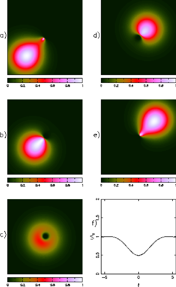
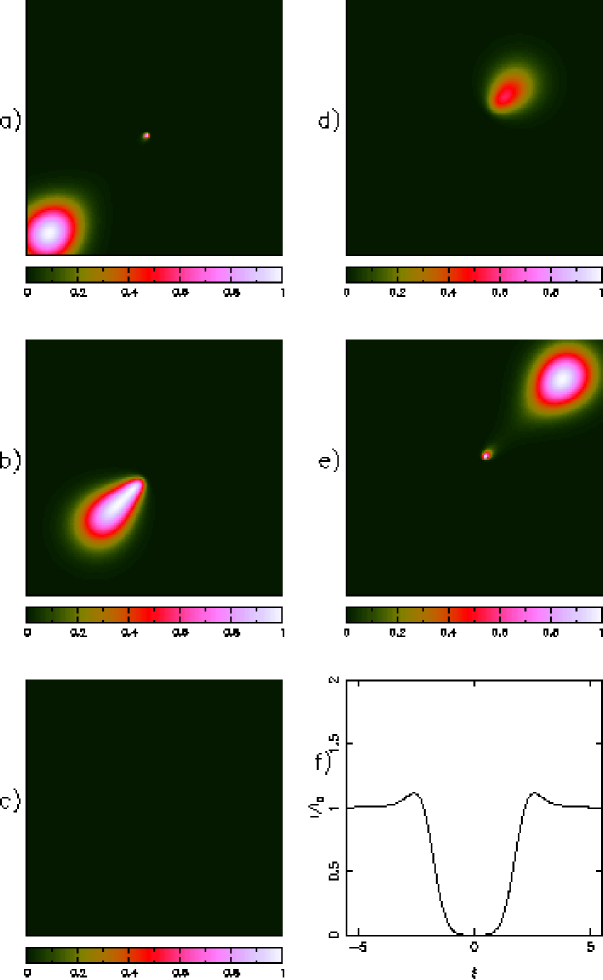
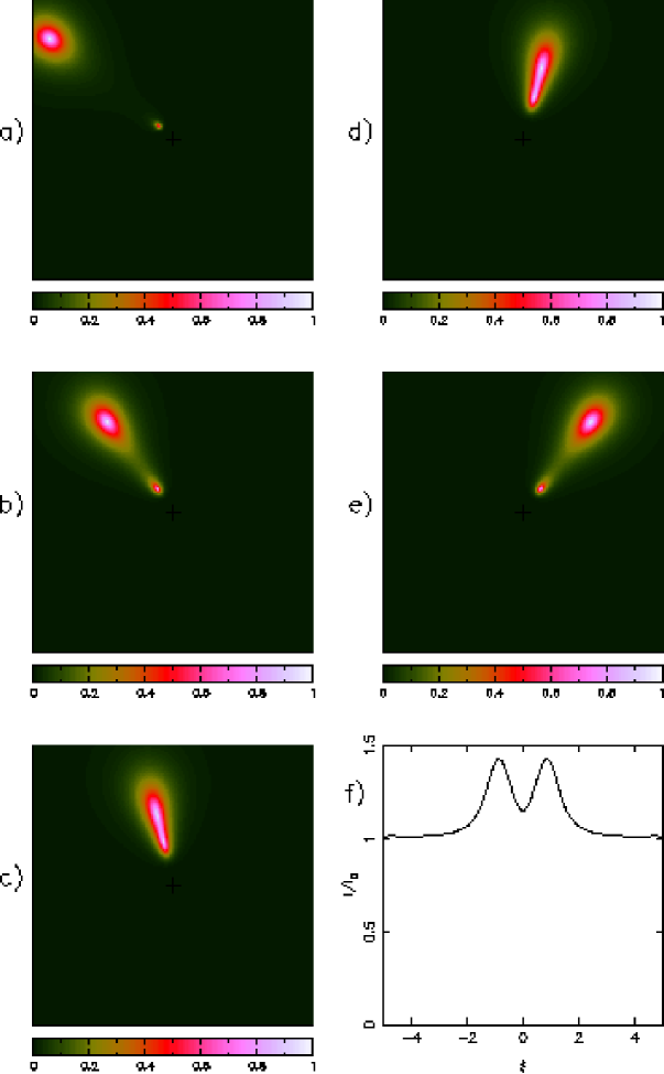
Source with exponential brightness distribution

We have for this brightness distribution $I(r)=I_{0}e^{-r/r_{0}}$. In the same manner as above, $R_{\rm S}$ is defined as radius, containing $90\%$ of total luminosity. In the same way as above, total luminosity

$$L(\infty)=\int_{0}^{\infty}e^{-{r}/{r_{0}}}2\pi r\,dr=2\pi r_{0}^{2}\,\,,$$ (3.55)

then

$$L(R)=\int_{0}^{R}e^{-{r}/{r_{0}}}2\pi r\,dr=2\pi\left[r_{0}^{2}-\left(R\,r_{0}+r_{0}^{2}\right)e^{-{R}/{r_{0}}}\right]\,\,,$$ (3.56)

and

$$\frac{L(R_{\rm S})}{L(\infty)}=0.9\,\,.$$ (3.57)

From where we find that effective radius relates to the parameter $r_{0}$ as

$$e^{-{R_{\rm S}}/{r_{0}}}\left(1+\frac{R_{\rm S}}{r_{0}}\right)=0.1\,\,.$$ (3.58)

Solution to this equation gives $R_{\rm S}/r_{0}\approx~{}3.89$. This profile is also normalized such that the maximum value of $I$ equals unity.

In Fig. 3.17 we display the images of the source with the exponential brightness profile and the corresponding light curve (frame f). The effective radius of the source is 1.5. The impact parameter here is $B_{0}=2.0$; the lensing regime corresponds to the one schematically depicted in Fig. 3.9. We see how shapes of the images change, becoming elongated and forming the radial arc (frames c and d).

Comparing light curves for sources with different brightness profiles

In Fig. 3.18 we compare light curves for three different radially symmetric source profiles: uniform, Gaussian and exponential, for two dimensionless source radii $\widetilde{R}=\widetilde{R}_{\rm S}^{\rm gauss}=\widetilde{R}_{\rm S}^{\rm expon}=0.1$ and $\widetilde{R}=\widetilde{R}_{\rm S}^{\rm gauss}=\widetilde{R}_{\rm S}^{\rm expon}=1.0$. As a reference curve we show the light curve of the point source. All curves are made for the impact parameter $B_{0}=0$. We can see larger noise in the uniform source curve, since the source with uniform brightness has an extremely sharp edge, whereas Gaussian and exponential sources are extremely smooth. Though we considered the sources with the same effective radius, we can see from the plot that for a small source size, the maximum magnification is reached by the source with exponential profile (upper panel). This is explained by the fact that this profile has a narrower central peak than the Gaussian.

For the larger source, this behaviour smoothens, though we still can see large differences in the light curves (bottom panel). Here the uniform source experiences darkening, while sources with other profiles only undergo demagnification.

Figure 3.18: Light curves for the point mass source (dashed line), source with constant surface brightness (solid), source with Gaussian brightness distribution (dash-dotted) and exponential brightness distribution (dotted) for two different effective dimensionless source radii, $0.1$ (upper panel) and $1.0$ (bottom panel).

3.3.6 Time scales of microlensing

Let the source have a transverse velocity ${\bf v}_{\rm s}$ measured in the source plane, the lens a transverse velocity ${\bf v}_{\rm l}$ measured in the lens plane, and the observer a transverse velocity ${\bf v}_{\rm obs}$ measured in the observer plane. The effective transverse velocity of the source relative to the critical curves with time measured by the observer is

$${\bf V}=\frac{1}{1+z_{\rm s}}{\bf v}_{\rm s}-\frac{1}{1+z_{\rm l}}\frac{D_{\rm s}}{D_{\rm l}}{\bf v}_{\rm l}+\frac{1}{1+z_{\rm l}}\frac{D_{\rm ls}}{D_{\rm l}}{\bf v}_{\rm obs}\,\,.$$ (3.59)

This effective velocity is such that for a stationary observer and lens, the position of the source will change in time according to $\delta\boldsymbol{\xi}={\bf V}\Delta t$.

We basically have two time scales of interest here. The first one is the typical rise time to a peak in the amplification. We can estimate that it corresponds to a displacement of $\Delta y\sim\widetilde{R}$ of the source across a critical line. The corresponding time scale is $\tau_{1}=t_{\rm v}\widetilde{R}$, with $t_{\rm v}$ given by (3.37). In terms of the physical source size $R=\xi_{0}\widetilde{R}$,

$$\tau_{1}=\frac{R}{V}\,\,,$$ (3.60)

where effective transverse velocity of the source $V$ is given by Eq. 3.59. The second time scale of interest is the time between two peaks $\tau_{2}$. For a point source we can estimate it as $\tau_{2}=t_{\rm v}\Delta$, where $\Delta$ is given in Eq. (3.44). For a source with radius $\widetilde{R}$ and impact parameter $B_{0}=0.0$ it can shown to be

$$\tau_{2}=t_{\rm v}\left(\Delta+\widetilde{R}\right)\,\,.$$ (3.61)

In Table 1 we list the time scales $\tau_{1}$ and $\tau_{2}$ for different values of a source radius, and the time delay between two images $\Delta t_{12}$ for the point source. The value of $V$ is estimated to be $V=5000$ km s^-1.

Table 1: Time scales for several source radii. $\tilde{R}$ is the dimensionless source radius, in units of Einstein angle, $|M|=1.0\,M_{\odot}$, redshift of the lens is $z_{\rm l}=0.1$, redshift of the source is $z_{\rm s}=0.5$, $\xi_{0}=5.42\times 10^{11}$ km is the normalized length unit in the source plane. The time scales correspond to apparent source velocity (see Eq. 3.59) $V=5000$ km s^-1.

$\widetilde{R}$	$R$ (pc)	$\Delta t_{12}$(sec)a	$\tau_{1}$ (yr)	$\tau_{2}$(yr)b
$0.0$	point source	$2.0\times 10^{-4}$	–	$6.78$
$0.01$	$1.07\times 10^{-4}$	–	$0.03$	$6.81$
$0.1$	$1.07\times 10^{-3}$	–	$0.34$	$7.11$
$1.0$	$1.07\times 10^{-2}$	–	$3.38$	$10.16$
$2.0$	$0.3\times 10^{-1}$	–	$6.75$	$13.6$

^a u=4.0 (definition in Eq. 3.29)
^b $B_{0}=0.0$

3.3.7 Concluding remarks

In these two sections we have explored the consequences of gravitational microlensing following from the existence of matter violating the energy conditions. We have also quantitatively analyzed, using numerical simulations, the influence of a finite size of the source on the gravitational lensing negative-mass event. We have thus enhanced and completed previous works where the focus was put on the point source light curves and no discussion was given concerning the shapes of images, actual simulations of microlensing events, time gain function, and other features presented here. Figs.  3.5, 3.8–3.11, 3.13–3.18 and Table 1 comprise our new results: a useful comparison arena where possible existence of wormholes or any other kind of negative mass compact objects can be observationally tested.

The next step would be to test these predictions using archival, current, and forthcoming observational microlensing experiments. The only search done up to now included the BATSE database of $\gamma$-ray bursts. There is still much unexplored territory in the gravitational microlensing archives. We suggest adaption of alert systems of these experiments in order to include the possible effects of negative masses as well. This would lead to a whole new world of discoveries.

3.4 Macrolensing

In this section we present a set of simulations showing macrolensing effects we could observe if a large amount of negative energy density exists in our universe. The physical systems could have an energy density equivalent to a total negative mass of the size of a galaxy or even a cluster of galaxies. In what follows, we used a background cosmology described by a FRW flat universe with $\Omega_{\rm m}=1$ and a zero cosmological constant. In all numerical computations a dimensionless Hubble parameter $h$ is put equal to 1 ($H_{0}=100\,h$ km sec^-1 Mpc^-1). The relationship $D_{\rm eff}=D_{\rm L}D_{\rm LS}D_{\rm S}^{-1}$ is a measure of the lensing efficiency of a given mass distribution. $D_{\rm eff}$ peaks, quite independently of the cosmological model assumed, at a lens redshift of $\sim 0.2-0.4$ for sources at a typical redshift $z_{\rm s}\sim 1-1.3$ [70]. To be more realistic, we placed the lens at a redshift of $z_{l}=0.3$ and generated a random sample of galaxies in the redshift range $0.3<z_{\rm source}<2.0$. The redshift distribution conserves their comoving number density. This number density and the projected sizes for these background sources were taken to be close to the Tyson population of faint blue galaxies [71]. The luminous area of each galaxy was taken to be a circular disk of radius $R$ with a uniform brightness profile and orientations of disk galaxies randomly placed in space. This was done by defining in the code the ellipticity $e$ ($e=(1-r)/(1+r)$, $r$ being the ratio of the minor axis to the major axis) and the position angle $\varphi$, and randomly chosing the values of $e$ from the range $0<e<0.7$ and the values of $\varphi$ from the range $0<\varphi<2\pi$.

We write the gravitational lens equation, which governs the mapping from the lens to the source plane, in dimensionless form

$$\mbox{\boldmath$\beta$}=\mbox{\boldmath$\theta$}\left[1+\frac{\theta^{2}_{\rm E}}{\theta^{2}}\right]\,\,.$$ (3.62)

The lens equation (3.62) describes a mapping ${\bf\theta}\mapsto{\bf\beta}$, from the lens to the source plane. For convenience, we redefine the lens plane as ${\bf x}$ and the source plane as ${\bf y}$. Then, Eq. (3.62) can be written as

$${\bf y}={\bf x}\left(1+\frac{\theta^{2}_{\rm E}}{x^{2}}\right),$$ (3.63)

where $x=|{\bf x}|=\sqrt{x_{1}^{2}+x_{2}^{2}}$.

We now consider a source, whose shape—either circular or elliptical—can be described by a function $\chi({\bf y})$. Curves of constant $\chi$ are the contours of the source. One can as well consider $\chi$ as a function of ${\bf x}$, $\chi({\bf y}({\bf x}))$, where ${\bf y}({\bf x})$ is found using the lens equation. Thus, all points ${\bf x}$ of constant $\chi$ are mapped onto points ${\bf y}$, which have a distance $\sqrt{\chi}$ from the centre of the source. If the latter contour can be considered an isophote of a source, one has thus found the corresponding isophotes of the images (see Section 3.3.3 for details on the algorithm).

3.4.1 Simulations results

In the first set of figures (Figs. 3.19-3.23), we show the results of our simulations. Some special precautions must be taken for the largest masses. The problem is that for a very massive lens the Einstein ring becomes very large. Since for the negative mass lensing all sources inside the double Einstein radius are shadowed (i.e. we can see the images of only those sources which are outside the double Einstein radius), if we were to use for lensing only the sources shown on the window, a fold-four symmetry pattern would appear (Fig. 3.24). Only the sources at the corners of the current window (and outside the double Einstein radius) are lensed. In order to solve this problem we have to consider also the sources from outside the current window; then the lensing picture is restored and the scale of the simulation is consistently increased. For this reason we increase the number of background galaxies in Figs. 3.21-3.23. We show this in detail in Figs. 3.24 and 3.25.

Figure 3.19: Left: Appearance of a background field of sources in a range of redshifts (see text) (200 galaxies, intrinsic radius 7 Kpc), when lensed by a negative mass of $|M|_{\rm lens}=1\times 10^{13}\,M_{\odot}$. Center: Unlensed background field. Right: Appearance of the same background field of galaxies when it is lensed by an equal amount of positive mass; redhsifts are the same as for the negative mass case.

Figure 3.20: Left: Appearance of a background field of sources (200 galaxies, intrinsic radius 10 Kpc), when it is lensed by a negative mass of $|M|_{\rm lens}=1\times 10^{14}\,M_{\odot}$. Center: As in Figure 3.19. Right: As in Figure 3.19.

Figure 3.21: Left: Appearance of a background field of sources (300 galaxies, intrinsic radius 15 Kpc), when it is lensed by a negative mass of $|M|_{\rm lens}=1\times 10^{15}\,M_{\odot}$. The simulation was made taking into account sources located within 1.2 of the size of the shown window. Center: As in Fig. 3.19. Right: As in Fig 3.19.

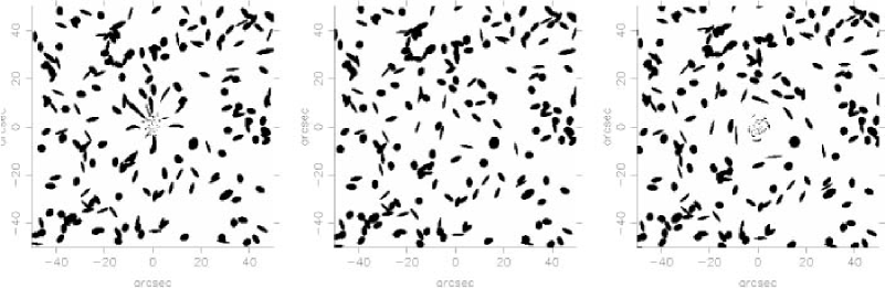
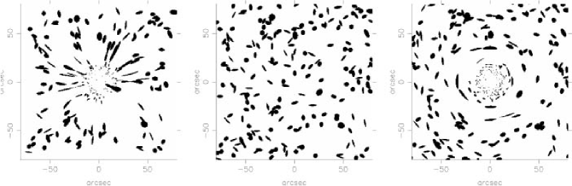
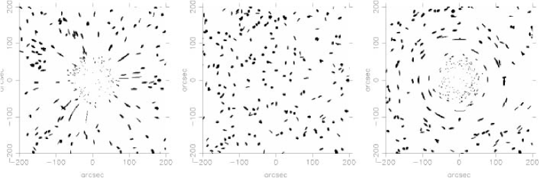
As a general feature of our simulations we can remark that, contrary to the standard positive mass case, where ring-like structures appear, the negative mass lensing produces finger-like, apparently “runaway" structures, which seem to escape from a central void. This is in agreement with the appearance of a central umbra in the case of a point-like negative mass lensing (see previous sections of this chapter). In the case of macrolensing, the umbra (central void) is maintained on a larger scale which, depending on the negative mass of the lens, can reach hundreds of acrsec in linear size. This umbra is always larger than the corresponding one generated in positive macrolensing (see Figures 3.19-3.23) and totally different in nature [60]. At least qualitatively, the existence of a macroscopic amount of negative mass lens mimics the appearance of galaxy voids.

Figure 3.22: Left: Appearance of a background field of sources (300 galaxies, intrinsic radius 50 Kpc), when it is lensed by a negative mass of $|M|_{\rm lens}=1\times 10^{16}\,M_{\odot}$. The simulation was made taking into account sources located within 1.2 of the size of the shown window. Center: As in Fig. 3.19. Right: As in Fig. 3.19.

Figure 3.23: Left: Appearance of a background field of sources (500 galaxies), intrinsic radius 60 Kpc, when it is lensed by a negative mass of $|M|_{\rm lens}=1\times 10^{17}\,M_{\odot}$. The simulation was actually made taking into account sources located within 1.5 of the size of the shown window. Center: As in Fig. 3.19. Right: As in Fig. 3.19.

Figure 3.24: The need for the increase of the background number of sources is shown by the appearance of a four-fold symmetric pattern, which occurs because only the galaxies at the corners of the left window are being affected by lensing effects. Axis are marked in arcseconds. See next figure.

Figure 3.25: Left: Appearance of a background field of circular sources (300 galaxies), each of them of 15 Kpc radius, when it is lensed by a negative mass of $|M|_{\rm lens}=1\times 10^{15}\,M_{\odot}$ with an Einstein angular radius equal to $\theta_{\rm E}=84$ arcsec. The dashed circle is the Einstein ring, the radial arcs are centered on it while the images inside it are demagnified. Here $z_{\rm lens}=0.4$, $z_{\rm source}=1.4$. The simulation was made taking into account sources located within 1.2 of the size of the shown window. Center: Background field in the absence of the lens, dashed circle is the double Einstein radius, all sources inside this radius are shadowed. Right: Macrolensing effects produced by a positive mass lens of $10^{15}\,M_{\odot}$, a dashed circle is the Einstein radius shown here for comparison, sources inside it are strongly lensed.

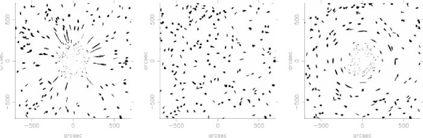
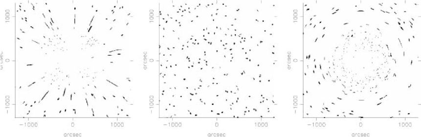
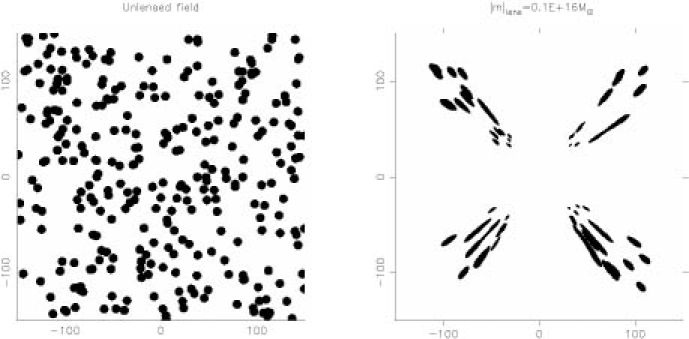
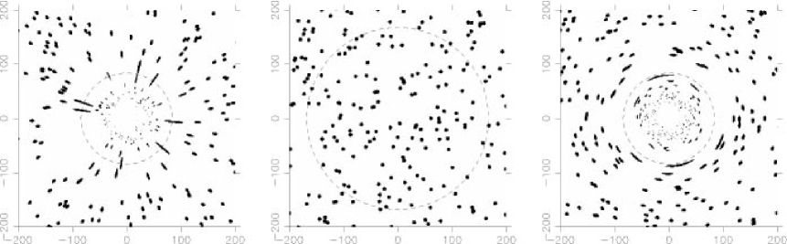
In order to explore the influence of the adopted redshift values, we turn now to the case where $z_{\rm sources}=0.08$ and $z_{\rm lens}=0.05$. The Bootes void is the closest void to us, and lies between the supercluster Corona Borealis ($z\approx 0.08$) and Hercules ($z\approx 0.03$) [74]. This serves as motivation for the selection of these redshift values. As an example of the results for different lens masses, we show in Figs. 3.26 and 3.27 the cases with $|M|_{\rm lens}=1\times 10^{14}\,M_{\odot}$ and $|M|_{\rm lens}=1\times 10^{16}\,M_{\odot}$.

Figure 3.26: Left: Appearance of a background field of sources (200 galaxies), each of them 5 Kpc radius, when it is lensed by a negative mass of $|M|_{\rm lens}=1\times 10^{14}\,M_{\odot}$ with an Einstein angular radius equal to $\theta_{\rm E}=47$ arcsec. Center: Unlensed background field. Right: Appearance of the same background field of galaxies when lensed by an equal amount of positive mass, located at the same redshift (see text).

Figure 3.27: Left: Appearance of a background field of sources (300 galaxies), each of them of 25 Kpc radius, when it is lensed by a negative mass of $|M|_{\rm lens}=1\times 10^{16}\,M_{\odot}$ with an Einstein angular radius equal to $\theta_{\rm E}=467$ arcsec. Center: As in Figure 3.26. Right: As in Figure 3.27.

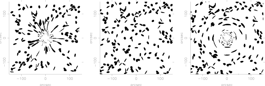
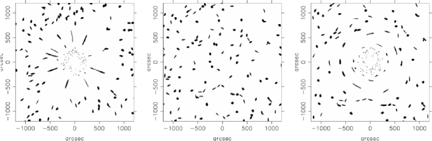
It is interesting to note that since the background population of galaxies is very dense, one would expect a lot of lensing in the standard model of cosmology. However, there is still a surprising dearth of candidates for (positive mass) lensed sources [75]. Some of the richest clusters do not display arcs in the deepest images. CL0016+16 ($z=0.56$), for instance, is one of the richest and strongest X-ray emitting clusters. It is rather extended on the sky and the light from many background sources should cross this cluster. Neither arcs nor arclets have been found, though weak lensing has been reported. This may be pointing towards a cautionary note: if the kind of finger-like structures displayed in our figures is not directly seen in its full pattern, that does not necessarily mean that they are absent. Even the presence of one radial arc (without tangential counter arc and/or tangential arcs) may be significant.

3.4.2 Concluding remarks

The null EC (NEC) is the weakest of the EC. Usually, it was considered that all reasonable forms of matter should at least satisfy the NEC. However, even the NEC and its averaged version (ANEC) are violated by quantum effects and semi-classical quantum gravity (quantized matter fields in a classical gravitational background). Moreover, it has recently been shown that there are also large classical violations of the energy conditions [76]. Here we have shown that disregarding the fundamental mechanism by which the EC are violated (e.g. fundamental scalar fields, modified gravitational theories, etc.), if large localized violations of NEC exist in our universe, we shall be able to detect them through cosmological macrolensing. Contrary to the usual case, where arc-like structures are expected, finger-like “runaway" filaments and a central void appear. In Figures 3.19-3.23 and  3.26-3.27 we compare the effects of negative masses with the case of macrolensing effects on background fields produced by equal amounts of positive mass located at the same redshift. The differences are obvious. These results make the cosmological macrolensing produced by matter violating the null energy condition observationally distinguishable from the standard situation. Whether large-scale violations of the EC, resulting in space-time regions with average negative energy density indeed exist in the universe can therefore be decided through observations.

Chapter 4 Gravitational Lensing as a Tool to Test Alternative Cosmologies

4.1 Introduction

Standard cold dark matter FRW cosmology presents serious theoretical and observational difficulties as an acceptable description of the Universe. For example, a study conducted on a sample of 256 ultra-compact sources [77] showed that the canonical CDM model ($\Omega_{0}=1$, $\Omega_{\Lambda}=0$) is ruled out at the 98.5% confidence level. An overview in the literature shows the existence of a growing body of work discussing alternative cosmologies [78]. The first motivation comes from the conflict between the age of the Universe and the age of the oldest stars in Galactic globular clusters. The ages of the globular clusters typically fall in the interval $12\,-\,14$ Gyr ([79], and references within), while measurements of the Hubble parameter were recently updated to $h=0.7\pm 0.1$ [80] with the value for the age in the interval 8.1 Gyr $\leq t_{0}\leq$ 10.8 Gyr. “The age problem” is even more acute if we consider its variant based on the age constraints from old galaxies at high redshifts [81].

Another important motivation is the cosmological constant problem. Historically, it was Einstein who introduced the $\Lambda$ term in his field equations in order to make them compatible with a static universe. The $\Lambda$ terms was introduced several times in cosmology but was discarded when improved data became available. Recently, observations by Perlmutter et al [82] and Riess et al [83] of more than 50 type Ia supernovae suggested Friedmann models with negative pressure matter, such as a cosmological constant, domain walls or cosmic strings [25, 84]. The main conclusion of these works was that the expansion of the universe is accelerating. Though a cosmic acceleration can also be accounted for by invoking inhomogeneity (though at a cost of the cosmological principle [85, 86]), a $\Lambda$-dominated model was revived again. The cosmological constant solves a lot of problems at once (for ex., [87]). It supplies the ‘missing matter’ required to make $\Omega_{\rm tot}=1$, it modifies CDM by putting more power on large scales, as is compatible with the CMBR anisotropy limits. It also removes the inconsistency between the age of the universe and that of the globular clusters for larger values of $H_{0}$. However, we face the problem that the upper limit of $\Lambda$ from observations ($\Lambda\lower 2.58334pt\hbox{$\;\buildrel<\over{\sim}\;$}10^{-56}$ cm^-2) is120 orders of magnitude below the value for the vacuum energy density predicted by quantum field theory [88, 89]. (It is customary to associate a positive cosmological constant $\Lambda$ with a vacuum density $\rho_{\rm v}\equiv\Lambda/8\pi G$.) According to gravitational lensing statistics, a universe with the a large cosmological constant should have more multiple-image systems than are actually observed. It was shown, for example, that HDF data may be incompatible with large $\Lambda$ [75].

These (and other) problems generated a lot of interest in an open FRW model with linear evolution of the scale factor, $a(t)\propto t$. This universe expands with a constant speed, hence the term coasting cosmology. Notable among such models is a recent idea of Allen [90], in which such a scaling results in an $SU(2)$ cosmological instanton dominated universe. Yet another possibility derives from the Weyl gravity theory of Manheim and Kazanas [91]. Here again the FRW scale factor appoaches a linear evolution at late times.

There are several motivations for investigating such models. Many of the problems of the standard model are naturally resolved in such a cosmology. Such a cosmology does not suffer from the horizon problem. Horizons occur in models with $a(t)\approx t^{\alpha}$ for $\alpha<1$. Linear evolution of a scale factor is supported in alternative gravity theories (eg. non-minimally coupled scalar-tensor theories), where it turns out to be independent of the matter equation of state. The scale factor in such theories does not constrain the matter density parameter, thereby curing the flatness problem. The age estimate in a coasting universe, deduced from the measurement of the Hubble parameter, is given by $t_{0}=1/H_{0}$. This is 50% greater than the age in standard CDM cosmology, thus making it comfortably concordant with the ages of globular clusters. Finally, a linear coasting cosmology independent of the equation of state of matter, is a generic feature in a class of models that attempt to dynamically solve the $\Lambda$ problem [92]. Such models have a scalar field non-minimally coupled to the large scale curvature of the universe. With the evolution of time, the non-minimal coupling diverges, the scale factor quickly approaches linearity and the non-minimally coupled field acquires a stress energy that cancels the vacuum energy in the theory. This model is consistent with nucleosynthesis in the early universe [93] and presents a good fit to the current SNE Ia data [94].

After the discovery of the first multipy imaged quasars, gravitational arcs and arclets, gravitational lensing has rapidly become one of the most promising tools for cosmology. It is now well known that gravitational lensing is a useful probe of the geometry of the universe. With the rapid growth of the number of lensed systems, proposals were made to apply the statistical analysis to the samples of lenses in order to extract the cosmological parameters. The use of gravitational lensing statistics as a cosmological tool was first considered in detail by Turner et al. [95] and Fukugita et al [96]. More recently, Kochanek [97] and Falco et al [98] have laid the groundwork for using gravitational lensing statistics for a detailed analysis of the extragalactic surveys. It has been pointed out [96, 99] that the expected frequency of multiple imaging lensing events for high-redshift sources is sensitive to cosmology. In view of the successfull results of the above mentioned works [93, 94], it is tempting to use this test to constrain the power index of the scale factor of a general power law cosmology, $a(t)\propto t^{\alpha}$. In the next section we consider constraints on this index. The expected number of lens systems depends upon the index $\alpha$ through the angular diameter distances. By varying $\alpha$, the number of lenses changes and on comparison with the observations we obtain constraints on $\alpha$.

One of the remarkable results of field theory is the existence of stable classical states of a field with non-vanishing energy. Such fields include topological solitons, domain walls, strings and monopoles. In addition to these field configurations, which are stabilized by their topological properties, non-topological solitons (NTS) produced by scalar fields have appeared in the literature and their relevance to cosmology has been assessed (for example, [100]). Variations on this theme include cosmic neutrino balls [101, 102], Q-balls [103] and soliton stars [104]. NTS are rendered stable by the existence of a conserved Noether charge carried by the fields confined to a finite region of space. The theory essentially contains an additive quantum number $N$, carried either by a spin-1/2 field $\psi$ (for example, fermion number), or a spin-0 complex field $\varphi$. In addition there is a scalar field $\sigma$ whose coupling gives $\varphi$ or $\psi$ a mass. The soliton contains the interior in which $\sigma\approx\sigma_{0}$, surrounded by a shell of width $\approx\mu^{-1}$, over which $\sigma$ changes from $\sigma_{0}$ to $0$. $\mu$ is the mass associated with $\sigma$. $\sigma=0$ and $\sigma=\sigma_{0}$ are two minima of the effective potential of the scalar field. The $N$-carrying field $\psi$, or $\varphi$, is confined to the interior where it is effectively massless at the local minimum of the potential, $\sigma=\sigma_{0}$. At the global minumum, $\sigma=0$, the field ($\psi$ or $\varphi$) has a non-vanishing mass, $m$. This leads to a stable configuration of massless particles trapped inside a region with $\sigma=\sigma_{0}$ separated from the true vacuum $\sigma=0$ by a wall of thickness $\approx\mu^{-1}$. Confinement occurs for all particle states that are not on-shell in the exterior region. The NTS is stable as long as the kinetic energy $E_{k}$ of the particles inside the bag is less than $E_{\rm free}$—the minimum on-shell energy in the exterior region. This was explicitly demonstrated by Lee and Wick [105, 106].

The role of scalar fields in effective gravity models stems from the classical work of Brans and Dicke. In these approaches the gravitational action is induced by a coupling of the scalar curvature with a function of a scalar field. Lee and Wick’s results can be carried over to a curved spacetime with a scalar curvature $R$ non-minimally coupled to $\sigma$ through arbitrary function $U(\sigma)$ in the class of theories described by the effective action

$$S=\int\sqrt{-g}\,d^{4}x\left[U(\sigma)R+\frac{1}{2}(\partial_{\mu}\sigma)^{2}-V(\sigma)+L_{\rm M}\right]\,\,.$$ (4.1)

Here $V(\sigma)$ is effective potential of a scalar field, $L_{\rm M}$ is the matter field(s) Lagrangian which includes a Higgs coupling of $\sigma$ to a fermion. Establishing $\sigma_{\rm in}$ and $\sigma_{\rm out}$ as the interior and exterior values of $\sigma$, the effective gravitational constant would be given by

$$G_{\rm eff}^{\rm in}=[U(\sigma_{\rm in}]^{-1}$$

and

$$G_{\rm eff}^{\rm out}=[U(\sigma_{\rm out}]^{-1}$$

If $U$ goes to infinity at some point, defined as $\sigma=0$ without loss of generality, the theory gives rise to a solution with a spatial variation of the effective gravitational constant, $G_{\rm eff}^{\rm out}=0$ and $G_{\rm eff}^{\rm in}=$constant. This would be a generic feature of a Lee-Wick solution in which the scalar field is non-minimally coupled to the scalar curvature. It would give rise to a stable “ball of gravity”.

A gravity ball is characterised by an effective refractive index in its interior. This would cause bending of light incident on it. The G-ball thus acts as a spherical lens. In the last section we investigate gravitational lensing of an empty gravity ball situated at a cosmological distance. The lens—gravity ball—has interesting features which are not shared by other known lenses. In the last section we examine gravitational lesning properties of this special kind of NTS solutions referred to as G-balls [107].

4.2 Gravitational lensing statistics as a test for coasting cosmology

4.2.1 Linear coasting cosmology

We consider a general power law cosmology with the scale factor given in terms of two parameters

$$a(t)=B\frac{c}{H_{0}}\left(\frac{t}{t_{0}}\right)^{\alpha}\,\,,$$ (4.2)

for an open FRW metric. However, the light propagates through the inhomogeneous rather than the averaged smooth spacetime. The light ray feels the local metric which deviates from the smooth FRW metric—FRW metric excludes gravitational lensing in principle. We may assume, however, that the relation between the affine distance of the null geodesic and the redshift of the source object in a clumpy universe is the same as in the FRW cosmology. This may be regarded as a mathematical expression of the assumption that the universe is described by FRW geometry on large scales (for the metric see Eq. 2.14).

Dimensionless Hubble parameter

The expansion rate of the universe is described by a Hubble parameter, $H=\dot{a}/a$. Using (4.2),

$$H(t)=\frac{\alpha}{t}\,\,.$$ (4.3)

The present expansion rate of the universe is defined by a Hubble constant, equal in our model to $H_{0}=\alpha/t_{0}$ (here and subsequently the subscript 0 on a parameter refers to its present value). With the usual definition of the redshift $z$

$$\frac{a_{0}(z)}{a(z)}=1+z$$ (4.4)

we obtain $t_{0}/t=(1+z)^{1/\alpha}$, and thus

$$H(z)=H_{0}(1+z)^{1/\alpha}\,\,.$$ (4.5)

The dimensionless Hubble parameter is

$$h(z)=\frac{H(z)}{H_{0}}=(1+z)^{1/\alpha}.$$ (4.6)

Present-day scale factor

We define the present ‘radius’ of the universe (4.2) as

$$a_{0}=B\frac{c}{H_{0}}\,\,.$$ (4.7)

Angular diameter distance

There are many ways to define a distance in cosmology—parallax distance, angular diameter distance, luminosity distance, proper motion distance, etc (see 2.2.4). It is the angular diameter distance that is relevant to the angular separation of images.

Consider a source at $r=r_{1}$ which emitted light at $t=t_{1}$. The observed angular diameter of the source, $\delta$, is related to the proper diameter of the source, D, by

$$\delta=\frac{D}{a(t_{1})\,r_{1}}\,\,.$$ (4.8)

The angular diameter distance $\rm D_{A}$ is defined to be

$${\rm D_{A}}(z)=\frac{D}{\delta}=a(t_{1})\,r_{1}=\frac{a_{0}r_{1}}{1+z},$$ (4.9)

where $r_{1}(z)$ is the coordinate distance to a redshift $z$. Angular diameter distance of a source at $z_{2}$ measured by an (fictitious) observer at $z_{1}$ is given by

$$D_{\rm A}(z_{1},z_{2})=\frac{a_{0}r_{12}}{1+z_{2}}\,\,.$$ (4.10)

Light travels on null geodesics, $ds^{2}=0$. If a comoving observer is at coordinates $(r_{0},\theta_{0},\phi_{0})$ at time $t_{0}$, the geodesics intersecting $r_{0}=0$ are lines of constant $\theta$ and $\phi$. Geodesic equation becomes

$$0=cdt^{2}-a^{2}(t)\frac{dr^{2}}{(1+r^{2})}$$ (4.11)

and the light signal emitted from coordinates $(r_{1},\theta,\phi)$ at time $t$ will reach the observer at time $t_{0}$ determined by

$$\int_{t}^{t_{0}}\frac{c\,dt^{\prime}}{a(t^{\prime})}=\int^{r_{1}}_{0}\frac{dr}{\sqrt{1+r^{2}}}$$ (4.12)

We can convert the integrals over $t$ into integrals over $z$ by differentiating (4.4),

$$\frac{dz}{dt}=-\frac{a_{0}}{a^{2}}\dot{a}=-\frac{a_{0}}{a}\frac{\dot{a}}{a}=-(1+z)H(z)\,\,,$$

to obtain

$$dt=-\frac{dz}{(1+z)H(z)}\,\,.$$ (4.13)

Thus, equation (4.12) becomes:

$$\int_{0}^{z}\frac{c\,dz}{H(z)(1+z)a}=\int_{0}^{r_{1}}\frac{dr}{\sqrt{1+r^{2}}}$$ (4.14)

Since $a_{0}/a=1+z$, we use it to obtain

$$\frac{c}{a_{0}}\int_{0}^{z_{1}}\frac{a_{0}\,dz}{H(z)(1+z)a}=\frac{c}{a_{0}}\int_{0}^{z_{1}}\frac{dz(1+z)}{H(z)(1+z)}=\frac{c}{a_{0}}\int_{0}^{z_{1}}\frac{dz}{H(z)}\,\,,$$ (4.15)

or, in terms of a dimensionless Hubble parameter $h(z)$, Eq. 4.12 becomes

$$\frac{c}{H_{0}a_{0}}\int_{0}^{z_{1}}\frac{dz}{h(z)}=\int_{0}^{r_{1}}\frac{dr}{\sqrt{1+r^{2}}}\,\,.$$

SSComoving Coordinate Distance $r$

For an open universe, $k=-1$, we obtain

$$\frac{c}{H_{0}a_{0}}\int_{0}^{z_{1}}\frac{dz}{h(z)}=\sinh^{-1}{r_{1}}\,\,.$$

Thus,

$$r_{1}=\sinh{\left[\frac{c}{H_{0}a_{0}}\int_{0}^{z_{1}}\frac{dz}{h(z)}\right]}\,\,.$$

SS$D_{\rm A}$ formulae If we take the value of $a_{0}$ from Eq. 4.7, we obtain

$$r_{1}=\sinh{\left[\frac{1}{B}\int_{0}^{z_{1}}\frac{dz}{h(z)}\right]}\,.$$ (4.16)

Then,

$$D_{\rm A}(z,\alpha)=\frac{Bc}{(1+z)H_{0}}\sinh{\left[\frac{1}{B}\int_{0}^{z_{1}}\frac{dz}{h(z)}\right]}\,,$$ (4.17)

with the integral

$$\int_{0}^{z_{1}}\frac{dz}{h(z)}=\frac{\alpha}{\alpha-1}\left\{(1+z)^{\frac{\alpha-1}{\alpha}}-1^{\frac{\alpha-1}{\alpha}}\right\}\,\,.$$

Finally, the distance formula is

$$D_{\rm A}(z,\alpha)=\frac{Bc}{(1+z)H_{0}}\sinh{\left[\frac{1}{B}\frac{\alpha}{\alpha-1}\left\{(1+z)^{\frac{\alpha-1}{\alpha}}-1^{\frac{\alpha-1}{\alpha}}\right\}\right]}\,\,.$$ (4.18)

The distance between two objects at different redshifts is:

$$D_{\rm A}(z_{1},z_{2},\alpha)=\frac{Bc}{(1+z_{2})H_{0}}\sinh{\left[\frac{1}{B}\frac{\alpha}{\alpha-1}\left\{(1+z_{2})^{\frac{\alpha-1}{\alpha}}-(1+z_{1})^{\frac{\alpha-1}{\alpha}}\right\}\right]}\,\,.$$ (4.19)

SSLimiting ($\alpha\rightarrow 1$) formulae

We know that $h(z)=(1+z)^{1/\alpha}$, with $\alpha\rightarrow 1$, thus, $h(z)=(1+z)$, then the integral

$$\int_{0}^{z}\frac{dz^{\prime}}{1+z^{\prime}}=\ln{(1+z)}\,\,,$$ (4.20)

and the Eq. 4.18 reduces to

$${\rm D_{A}}(z)=\frac{Bc}{H_{0}}\frac{1}{1+z}\sinh{\left[\frac{1}{B}\ln{(1+z)}\right]}=\frac{Bc\left[(1+z)^{2/B}-1\right]}{2\,H_{0}(1+z)^{\frac{B+1}{B}}}\,\,.$$ (4.21)

The distance between two objects at different redshifts is, accordingly,

$${\rm D_{A}}(z_{1},z_{2})=\frac{Bc}{2H_{0}}\frac{\left[(1+z_{2})^{2/B}-(1+z_{1})^{2/B}\right]}{(1+z_{1})^{1/B}(1+z_{2})^{\frac{B+1}{B}}}\,\,.$$ (4.22)

Look-back time

The look-back time, $\Delta t=|t-t_{0}|$, is the difference between the age of the universe when a particluar light ray was emitted and the age of the universe now:

$$\Delta t(a;a_{0})=\int_{a}^{a_{0}}\frac{da}{\dot{a}(a)}\,\,\,.$$ (4.23)

We can obtain the expression for the look-back time from Eq. 4.13 and Eq. 4.6. Since we define $t_{0}$ as zero and time is increasing as we look back, we drop the negative sign in that expression. Thus,

$$\frac{dt}{dz}=\frac{1}{H_{0}(1+z)^{\frac{\alpha+1}{\alpha}}}\,\,,$$ (4.24)

and finally the expression we seek is:

$$\frac{c\,dt}{dz_{\rm L}}=\frac{c}{H_{0}(1+z_{\rm L})^{\frac{\alpha+1}{\alpha}}}\,\,.$$ (4.25)

4.2.2 Basic equations of gravitational lensing statistics

Given a lens model, the number counts of galaxies–lenses and their properties, we compute the probability $p_{i}$ that quasar $i$ is lensed and the probability $p_{i}(\Delta\theta_{i})$ that quasar $i$ is lensed and has image separation $\Delta\theta_{i}$. We shall consider only early types of galaxies, elliptical and lenticulars, E/S0, neglecting the contribution of spirals as lenses. This is because the velocity dispersion $v$ of spirals is small compared to E/S0 galaxies, outweighing the larger number density. The numbers of E/S0 and spirals are roughly 30% and 70%, respectively, whereas in our adopted sample the velocity dispersion of ellipticals is about 200 km s^-1 and that of spirals is about 130 km s^-1 [108]. The calculations for the lensing statistics depend strongly on this quantity, since the lensing optical depth goes as the fourth power of the velocity dispersion (see Eq. 4.45).

It is increasingly clear [97] that E/S0 galaxies are effectively singular. The almost uniform absence of central images in the observed lenses and models of individual lenses imply core radius smaller than 100 $h^{-1}$ pc and essentially suggest that the galaxy lenses are nearly singular [24, 109]. We will model the lensing galaxies as singular ($=$ zero core radius) isothermal spheres (SIS). The detailed lensing properties of singular isothermal spheres are described in Section 2.3.5. Here we simply state the most important relations for the present calculations. A SIS lens with a velocity dispersion $v$ at a redshift $z_{\rm L}$ will produce two images of a quasar at a redshift $z_{\rm S}$ separated by an angle $\Delta\theta$

$$\Delta\theta=2\alpha_{\rm d}\frac{D_{\rm LS}}{D_{\rm S}}\,\,,$$ (4.26)

if angular position of the source is less than the critical angle $\beta_{\rm cr}\equiv\alpha_{\rm d}D_{\rm LS}/D_{\rm S}$. The deflection angle, $\alpha_{\rm d}$, is given for all impact parameters as:

$$\alpha_{\rm d}=4\pi\left(\frac{v}{c}\right)^{2}\,\,.$$ (4.27)

The angular separation of the two images is independent of the impact parameter as long as it is small enough to produce two images. The critical impact parameter is defined by $a_{\rm cr}\,\equiv\,D_{\rm L}\beta_{\rm cr}$ or, with the help of the previous definitions,

$$a_{\rm cr}=4\pi\left(\frac{v}{c}\right)^{2}\frac{D_{\rm L}D_{\rm LS}}{D_{\rm S}}\,\,.$$ (4.28)

The quasars are treated as point sources of radiation. We assume that no evolution of galaxies or quasars with cosmic time (quasar evolution is irrelevant, since the quasar redshift distribution will be drawn from observed samples). In other words, the comoving number density of lenses is conserved

$$n_{\rm L}=n_{0}(1+z_{\rm L})^{3}\,\,,$$ (4.29)

where $n_{0}$ is an average comoving density measured at the present epoch. Merging between galaxies and infall of surrounding mass onto galaxies are two posible processes that can change the comoving density of galaxies and/or their mass. Under the generic relation between the velocity dispersion and mass of early-type galaxies, Rix et al [110] and Mao & Kochanek [111] found that merging and/or evolution does not significantly change the statistics of lensing.

Cross-section and optical depth of lensing.

The cross-section $\sigma$ for "strong" lensing events is given by$\sigma=\pi a_{\rm cr}^{2}$. Using (4.27) and the definitions from the previous subsection, we write the cross-section as

$$\sigma=16\pi^{3}\left(\frac{v}{c}\right)^{4}\left(\frac{D_{\rm L}D_{\rm LS}}{D_{\rm S}}\right)^{2}\,\,.$$ (4.30)

The cross-section is largest approximately halfway in the distance between the source and the observer; and $\sigma$ vanishes at the two endpoints. To find the average effect on an image passing within $a_{\rm cr}$ of a mass (“scoring a hit"), we average over the cross-section to find the mean image separation as

$$\overline{\Delta\theta}=8\pi\left(\frac{v}{c}\right)^{2}\frac{D_{\rm LS}}{D_{\rm S}}\,\,.$$ (4.31)

The differential probability (or the optical depth) $d\tau$ that a line of sight intersects a galaxy-lens at $z_{\rm L}$ in traversing the path of $dz_{\rm L}$ from a population with number density $n_{\rm L}$ is given by a ratio of differential light travel distance $cdt$ to its mean free path between successive encounters with galaxies, $1/n_{\rm L}(z)\sigma$,

$$d\tau=n_{\rm L}(z)\sigma\frac{cdt}{dz_{\rm L}}dz_{\rm L}\,\,.$$ (4.32)

For our case $n_{\rm L}(z)$ is given by (4.29) and the quantity $cdt/dz_{\rm L}$ is obtained in the previous section (Eq. 4.25). Substituting for $\sigma$ and $n_{\rm L}(z)$, we get

$$d\tau=\frac{16\pi^{3}}{c^{4}}(1+z_{\rm L})^{3}\langle n_{0}v^{4}\rangle\left(\frac{D_{\rm L}D_{\rm LS}}{D_{\rm S}}\right)^{2}\frac{cdt}{dz_{\rm L}}dz_{\rm L}\,\,.$$ (4.33)

Assuming that the brightness distribution of galaxies at any given redshift is described by a Schechter function, the comoving density of galaxies at redshift $z$ and with luminosity between $L$ and $L+dL$ is

$$\Phi(L,z)dL=n_{*}(z)\left(\frac{L}{L_{*}(z)}\right)^{\hat{\alpha}}\exp{\left(-\frac{L}{L_{*}(z)}\right)}\frac{dL}{L_{*}(z)}\,\,.$$ (4.34)

The parameter $n_{*}(z)$ is the average comoving density, $L_{*}(z)$ is the characteristic luminosity at which the luminosity function exhibits a rapid change in the slope in the $\log{n},\,\log{L}$)-plane and $\hat{\alpha}$ gives the slope of the luminosity function in the ($\log{n},\,\log{L}$)-plane, when $L\ll L_{*}$. The comoving number density of galaxies, characteristic luminosity and mass of a galaxy at any redshift remain constant, therefore, $n_{*}(z)=n_{*}(0)=\mbox{constant}$ and $L_{*}(z)=L_{*}(0)=\mbox{constant}$. “0" refers to present-day values. This is the most commonly used luminosity function for early type galaxies. Thus, Eq. 4.34 becomes

$$\Phi(L,z=0)\,dL=n_{*}\left(\frac{L}{L_{*}}\right)^{\hat{\alpha}}\exp{\left(-\frac{L}{L_{*}}\right)}\,\frac{dL}{L_{*}}\,\,.\,$$ (4.35)

where $n_{*}$, $\hat{\alpha}$ and $L_{*}$ are the normalization factor, index of the faint-end-slope and the characteristic luminosity at the present epoch, respectively. These values are fixed in order to fit the current luminosities and densities of galaxies. From Eq. 4.33 and Eq. 4.35 we have

$$\langle n_{0}v^{4}\rangle=v_{*}^{4}n_{*}\int_{0}^{\infty}\left(\frac{L}{L_{*}}\right)^{\hat{\alpha}}\exp{\left(-\frac{L}{L_{*}}\right)}\,\frac{dL}{L_{*}}\left(\frac{v}{v_{*}}\right)^{4}\,.$$ (4.36)

We assume the velocity dispersion $v$ is related to the luminosiy $L$ by the empirical Faber-Jackson relation for E/S0 galaxies:

$$\left(\frac{L}{L_{*}}\right)=\left(\frac{v}{v_{*}}\right)^{\gamma}\,\,.$$ (4.37)

Therefore, Eq. (4.36) becomes

$$\langle n_{0}v^{4}\rangle=v_{*}^{4}n_{*}\int_{0}^{\infty}\left(\frac{L}{L_{*}}\right)^{4\hat{\alpha}+\gamma}\exp{\left(-\frac{L}{L_{*}}\right)}\frac{dL}{L_{*}}\,\,.$$ (4.38)

By integrating it over the luminosity function at redshift $z$, we obtain the differential probability

$$d\tau=\frac{16\pi^{3}}{c^{4}}(1+z_{\rm L})^{3}n_{*}v_{*}^{4}\Gamma\left(\hat{\alpha}+\frac{4}{\gamma}+1\right)\left(\frac{D_{\rm L}D_{\rm LS}}{D_{\rm S}}\right)^{2}\frac{cdt}{dz_{\rm L}}dz_{\rm L}\,\,$$ (4.39)

where $\Gamma$ is the normal gamma function. If we define the ‘dimensionless’ image splitting as $\phi=\Delta\theta/8\pi\left(v_{*}/c\right)^{2}$, we can find the differential optical depth of lensing in traversing $dz_{\rm L}$ with the angular separation between $\phi$ and $\phi+d\phi$ as $\frac{d^{2}\tau}{dz_{\rm L}d\phi}d\phi dz_{\rm L}$. Using luminosity-velocity relation (Eq. 4.37), we obtain the relation

$$\frac{L}{L_{*}}=\left(\frac{D_{\rm S}}{D_{\rm LS}}\phi\right)^{\gamma/2}\,\,.$$ (4.40)

Taking the differential,

$$\frac{dL}{L_{*}}=\frac{\gamma}{2}\left(\frac{D_{\rm S}}{D_{\rm LS}}\phi\right)^{\gamma/2}\frac{d\phi}{\phi}\,\,.$$ (4.41)

Returning to the Eq. 4.33), we write $d\tau/dz_{\rm L}$ as

$$\frac{d\tau}{dz_{\rm L}}=n_{\rm L}(z)\frac{16\pi^{3}}{c^{4}}v^{4}\left(\frac{D_{\rm L}D_{\rm LS}}{D_{\rm S}}\right)^{2}\frac{cdt}{dz_{\rm L}}\,\,.$$ (4.42)

The differential optical depth of lensing in traversing $dz_{\rm L}$ with the angular separation between $\phi$ and $\phi+d\phi$ is

$$\hskip-57.81621pt\int_{0}^{\infty}\frac{d^{2}\tau}{dz_{\rm L}d\phi}d\phi=$$

(4.43)

$$n_{*}v_{*}^{4}\int_{0}^{\infty}\left(\frac{L}{L_{*}}\right)^{\hat{\alpha}}\exp{\left(-\frac{L}{L_{*}}\right)}\frac{dL}{L_{*}}\left(\frac{L}{L_{*}}\right)^{4/\gamma}\left(1+z_{\rm L}\right)^{3}\frac{16\pi^{3}}{c^{4}}\left(\frac{D_{\rm L}D_{\rm LS}}{D_{\rm S}}\right)^{2}\frac{cdt}{dz_{\rm L}}\,\,.$$

Using the relations (Eq. 4.41), we obtain

$$\frac{d^{2}\tau}{dz_{\rm L}d\phi}d\phi dz_{\rm L}=$$

$$F^{*}(1+z_{\rm L})^{3}\frac{H_{0}}{c}\frac{\gamma/2}{\Gamma\left(\hat{\alpha}+1+\frac{4}{\gamma}\right)}\frac{cdt}{dz_{\rm L}}\left(\frac{H_{0}D_{\rm L}D_{\rm LS}}{c\,\,D_{\rm S}}\right)^{2}\left(\frac{D_{\rm S}}{D_{\rm LS}}\phi\right)^{\frac{\gamma}{2}(\hat{\alpha}+1+\frac{4}{\gamma})}\exp{\left[\left(-\frac{D_{\rm S}}{D_{\rm LS}}\phi\right)^{\frac{\gamma}{2}}\right]}\frac{d\phi}{\phi}dz_{\rm L}\,.$$

Here we have introduced the useful dimensionless quantity $F^{*}$ which measures the effectiveness of matter in producing multiple images [95]

$$F^{*}\equiv\frac{16\pi^{3}}{cH_{0}^{3}}n_{*}v_{*}^{4}\Gamma\left(\hat{\alpha}+1+\frac{4}{\gamma}\right)\,\,.$$ (4.45)

Lens and source parameters.

The variables relating galaxy numbers counts and the isothermal lens model are the number density of E/S0 galaxies $n_{*}$, the Schechter function slope $\hat{\alpha}$, the Faber-Jackson exponent $\gamma$ and the velocity dispersion of the dark matter for an $L_{*}$ galaxy $v_{*}$. The Schechter function slope $\hat{\alpha}$ controls the relative number of low- and high-mass galaxies. We use the following list of lens parameters for our calculations [108]:

$Survey$	$\alpha$	$\gamma$	$v^{*}(Km/s)$	$\phi^{*}(Mpc^{-3})$	$F^{*}$
$LPEM$	$+0.2$	$4.0$	$205$	$3.2\times 10^{-3}$	$0.010$

We consider a sample of 867 ($z>1$) high luminosity optical quasars which include 5 lensed quasars ($1208+1011$, H $1413+117$, LBQS $1009+0252$, PG $1115+080$, $0142+100$). This sample is taken from optical lens surveys, such as the HST Snapshot survey, the Crampton survey, the Yee survey, Surdej survey, the NOT Survey and the FKS survey [112]. The lens surveys and quasar catalogues usually use V magnitudes, so we transform $m_{V}$ to a B-band magnitude using $B-V=0.2$ [113].

We make two corrections to the optical depth to get the lensing probability: magnification bias and selection function.

Magnification bias.

Lensing increases the apparent brightness of a quasar causing over-representation of multiply imaged quasars in a flux-limited sample. This effect is called magnification bias. It is an enhancement of the probability that a quasar is lensed, that is why we have to include this correction in the probability function. The bias for a quasar at a redshift $z$ with apparent magnitude $m$ is given as [96, 114, 97]

$$B(m,A_{\rm lim},A_{2},z)=\left(\frac{dN(m.z)}{dm}\right)^{-1}\int_{A_{\rm lim}}^{A_{2}}\frac{dN(m_{\rm A},z)}{dm}p(A)dA\,\,.$$ (4.46)

Here $A$ is the total magnification, $A_{\rm lim}$ the magnification at which the images have the minimum detectable flux ratio (for a SIS model, $A_{\rm lim}=A_{0}=2$), $m_{\rm A}=m+2.5\log{A}$ is the lensing enhanced magnitude and $p\,(>A)$ is the probability distribution for the two images having a total magnification larger than $A$, $p(A)=8/A^{3}$ for a SIS model. We can allow the upper limit on magnification $A_{2}$ to be infinite, but in practice we set it to be $A_{2}=10^{4}$. For the quasar apparent magnitude number counts we use Kochanek’s broken power law [97]

$$\frac{dN(m,z)}{dm}\propto\left(10^{-a(m-m_{0}(z))}+10^{-b(m-m_{0}(z))}\right)^{-1}\,\,,$$ (4.47)

where the bright-end slope index $a$ and faint-end slope index $b$ are constants and the break magnitude $m_{0}$ evolves with redshift as

$$m_{0}(z)=\left\{\begin{array}[]{lcl}m_{0}+(z+1)&\mbox{if}&z<1\\ m_{0}&\mbox{if}&1<z<3\\ m_{0}-0.7(z-3)&\mbox{if}&z>3\,\,.\end{array}\right.$$

Fitting this model to the quasar luminosity function data in [115] for $z>1$, Kochanek finds that the ‘best model’ has $a=1.07$, $b=0.27$ and $m_{0}=18.92$ at B magnitude. Thus, magnitude corrected probability $p_{i}$ for the quasar $i$ with apparent magnitude $m_{i}$ and redshift $z_{i}$ to get lensed is $p_{i}=\tau(z_{i})B(m_{i},A_{\rm lim},A_{2},z_{i})$.

Selection function.

Selection effects are caused by limitations on dynamic range, limitations on resolution and presence of confusing sources such as stars. In the SIS model the selection function is modeled by a maximum magnitude difference $\Delta m(\theta)$ that can be detected for two images separated by $\Delta\theta$. This is equivalent to a limit on the flux ratio between two images $f=10^{0.4\Delta m(\theta)}$. The total magnification becomes $A_{f}=A_{0}(f+1)/(f-1)$. So, the survey can only detect lenses with magnifications greter than $A_{f}$. This sets the lower limit on magnifications and in the bias function $A_{\rm lim}$ gets replaced by $A_{f}$. To get selection function corrected probabilities, we divide our sample into two parts: the ground based surveys and the HST Snapshot survey and use the selection function for each survey as suggested by Kochanek [114].

The corrected lensing probability and image separation distribution function for a single source at redshift $z_{\rm S}$ are given as [97]

$$p^{{}^{\prime}}_{i}(m,z)=p_{i}\int\frac{d(\Delta\theta)\,p_{c}(\Delta\theta)\emph{B}(m,z,M_{f}(\Delta\theta),M_{2})}{\emph{B}(m,z,M_{0},M_{2})},$$ (4.48)

and

$$p^{{}^{\prime}}_{ci}=p_{ci}(\Delta\theta)\,\frac{p_{i}}{p_{i}^{{}^{\prime}}}\,\frac{\emph{B}(m,z,M_{f}(\Delta\theta),M_{2})}{\emph{B}(m,z,M_{0},M_{2})}\,\,,$$ (4.49)

where

$$p_{c}(\Delta\theta)=\frac{1}{\tau(z_{S})}\,\int_{0}^{z_{S}}\frac{d^{2}\tau}{dz_{L}d(\Delta\theta)}\,dz_{L}\,\,.$$ (4.50)

Equation (4.49) defines the configuration probability. It is the probability that the lensed quasar $i$ is lensed with the observed image separation.

4.2.3 Testing the model against observations

The above basic equations were used to perform the following test:

• The sum of the lensing probabilities $p_{i}^{{}^{\prime}}$ for the optical QSOs gives the expected number of lensed quasars, $n_{\rm L}=\sum\,p_{i}^{{}^{\prime}}$. The summation is over the given quasar sample. We look for those values of the parameter for which the adopted optical sample has exactly five lensed quasars (that is, those values of the parameters for which $n_{\rm L}=5$).

  We started with a two parameter fit. We allowed $\alpha$ to vary in the range ($0.0\leq\alpha\leq 2.0$) and $B$ to vary in the range ($0.5\leq B\leq 10.0$). We observe that for $B\geq 1$, $D_{A}$ becomes independent of it (as is also obvious from equation (4.18)). In the previous works constraining power law cosmology [93, 94], the value of $B=1$ was found to be compatible with the observations. Incidentally, we can estimate the present scale factor of the universe as $a_{0}\approx c/H_{0}$. Therefore, we used $B=1$ in further analysis.

  Fig. 4.1 shows the predicted number of lensed quasars for the above specified range of $\alpha$. We obtained $n_{L}=5$ for $\alpha=1.06$. We further generated $10^{4}$ data sets using bootstrap method (see description in [116]) and found the best fit for $\alpha$ for each data set in order to obtain error bars on $\alpha$. We finally obtained $\alpha=1.09\pm 0.3$.

  

  Figure 4.1: Predicted number of lensed quasars $n_{\rm L}$ in the adopted optical quasar sample, with $\Delta\theta\leq 4^{\prime\prime}$, vs. power index $\alpha$.

The maximum likelihood analysis was also performed [116] to determine the value of $\alpha$, for which the observed sample becomes the most probable observation. It was found that $0.85\leq\alpha\leq 1.56$ at $1\sigma$ ($68\%$ confidence level), and $0.65\leq\alpha\leq 2.33$ at $2\sigma$ ($95.4\%$ confidence level). It is also interesting to notice that for a general power law cosmology the simplest constraint on $\alpha$ comes from the relation $\alpha=H_{0}t_{0}$ (Eq. 4.3). With updated value of $H_{0}=70\pm 7$ km/sec/Mpc [80] and $t_{0}=14\pm 2$ Gyr [117], this constraint gives $\alpha=0.98\pm 0.25$.

4.2.4 Concluding remarks

In this section we discussed the general power law cosmology and the ways to constraint its power index. We have derived angular diametere distances for this cosmology. We described the general formulation of the gravitational lensing statistics and used it to constraint the parameters for that cosmology. These results together with other tests were used in [4] in the combined form and the conclusion made was that open linear coasting cosmology, $a(t)=t$, is consistent with the present observations.

4.3 Gravity balls as gravitational lenses

4.3.1 Gravity ball as a NTS solution

Here we will discuss the general formalism of the problem for a spherically symmetric system consisting of fermion field $\psi$, scalar field $\sigma$ and gravitational field $g_{\mu\nu}$. We follow the theory presented by Sethi and Lohiya [107]. Gravity balls are the NTS solutions of the field equations arising from (1)

$$U(\sigma)[R^{\mu\nu}-\frac{1}{2}g^{\mu\nu}R]=-\frac{1}{2}\left[T^{\mu\nu}_{\omega}+T^{\mu\nu}_{\sigma}+T^{\mu\nu}_{\sigma,\psi}+T^{\mu\nu}_{\psi}+2U(\sigma)^{;\mu;\nu}-2g^{\mu\nu}U(\sigma)^{;\lambda}_{;\lambda}\right]$$ (4.51)

$$g^{\mu\nu}\sigma_{;\mu;\nu}+\frac{\partial{V}}{\partial{\sigma}}-R\frac{\partial{U}}{\partial{\sigma}}=0$$ (4.52)

Here $T^{\mu\nu}_{\sigma}$, $T^{\mu\nu}_{\psi}$, $T^{\mu\nu}_{\sigma,\psi}$ and $T^{\mu\nu}_{\omega}$ are energy momentum tensors constructed from action for the scalar field, the fermion field, together with its Higgs coupling to $\sigma$, and the rest of the matter fields, respectively. We consider an NTS with the scalar field held to a value $\sigma_{0}$ in the interior and making a fast transition to $\sigma=0$ outside a thin shell. Thus, we have essentially three regions: (i) the interior of a soliton ($r<R_{0}$); (ii) a shell of thickness $\sim\mu^{-1}$ and surface energy density $s\approx\mu\sigma_{0}^{2}/6$; and (iii) the exterior ($r>R_{0}$). The total energy of a NTS has contributions from: (1) the surface tension energy $E_{s}\approx sR_{0}^{2}\,$; (2) the energy of the fermions $E_{f}\approx N^{4/3}/R_{0}$ and; (3) the volume energy $E_{V}\approx V(\sigma_{\rm in})R_{0}^{3}$. For the degenerate case $V(\sigma_{\rm in})=0$, a NTS has total mass constrained by the stability against gravitational collapse to a value determined by the surface tension $s$. The soliton mass, obtained by minimizing the total energy, is $M=12\pi sR_{0}^{2}$. For $s\sim(\mbox{MeV})^{3}$ and $N\approx 10^{75}$, the size of the NTS is of the order of tens of kiloparces, while it is still away from the Schwarzschild bound. For configurations with $R$ much greater than the Schwarzschild radius, the effects of gravity can be treated as a small perturbation. Thus, the form of the metric for the NTS satisfies a weak-field approximation.

A. Interior: $r<R_{0}+{\cal O}\left(\mu^{-1}\right)$.

The metric inside is described as

$$ds^{2}=e^{2u(r)}\,dt^{2}-e^{2v(r)}\,dr^{2}-r^{2}[d\theta^{2}+\sin^{2}\theta\,d\varphi^{2}]$$ (4.53)

The interior metric has one specific solution: $v=-\hat{C}r^{2}/6$ and

$$u=u_{0}+\frac{r^{2}}{2}\left[\frac{\tilde{C}}{2}+\frac{\hat{C}}{3}\right]\;,$$ (4.54)

with $\tilde{C}$ and $\hat{C}$—constants depending on the fermionic energy inside the soliton. In the weak field approximation used here we consider the interior with

$$ds^{2}\approx e^{2u_{0}}\,dt^{2}-dr^{2}-r^{2}\left[d\theta^{2}+\sin^{2}{\theta\,d\varphi^{2}}\right]$$ (4.55)

B. Exterior: $r>R_{0}+{\cal O}\left(\mu^{-1}\right)$.

In the exterior region we have essentially a Minkowskian metric

$$ds^{2}=dt^{2}-dr^{2}-r^{2}\left[d\theta^{2}+\sin^{2}{\theta\,d\varphi}^{2}\right]$$ (4.56)

To be consistent with the observations we will see that the $u_{0}$ has to be a small negative constant. The propagation of light inside the G-ball is equivalently described by using the Fermat principle with the effective refraction index $n_{\rm eff}$ inside the ball given by $n_{\rm eff}=1-u_{0}$. This gives straight trajectories of light rays inside the ball. But since outside the ball $n_{\rm eff}=1$, we see that G-ball behaves as a spherical lens (deflection of light occurs only at the boundaries).

4.3.2 Lens model for a G-ball and lensing properties

We restrict our discussion to a cosmological model which is a variant of a Milne universe [107] with a scale factor $a(t)=t$. In this cosmology angular diameter distances are given by

$$D_{\rm L}=\frac{cz_{\rm l}}{2H_{0}}\frac{(2+z_{\rm l})}{(1+z_{\rm l})^{2}}\,,$$

$$D_{\rm S}=\frac{cz_{\rm s}}{2H_{0}}\frac{(2+z_{\rm s})}{(1+z_{\rm s})^{2}}\,,$$

$$D_{\rm LS}=\frac{cz_{\rm ls}}{2H_{0}(1+z_{\rm l})}\frac{(2+z_{\rm ls})}{(1+z_{\rm ls})^{2}}\,\,.$$ (4.57)

with

$$z_{\rm ls}=\frac{z_{\rm s}-z_{\rm l}}{1+z_{\rm l}}\,\,,$$

and $H_{0}=100\,h$ km s^-1 Mpc^-1. Subscripts ‘l’, ‘s’ and ‘ls’ stand for lens, source and lens-source, respectively.

We consider the gravity ball to be of the size of a typical cluster of galaxies at the cosmological distance and embedded in empty space region with no matter concentrations close to it. The deflector is transparent. We also assume a thin-lens approximation, since all the deflection occurs within $\Delta z\leq\pm R_{\rm ball}$; the extent of the deflector is thus taken to be small compared with its distance from both the observer and the source. Typical distances from us to the cluster at $z=0.3$ and to the source at $z=1$ are $\sim 1\,\,Gpc$ and $\sim 2\,\,Gpc$, respectively, while $R_{\rm ball}\approx 0.5$ to $1$ Mpc. We consider deflection angles to be small. We also assume that the source, lens, and observer are stationary with respect to comoving coordinates.

The magnification of images in the axisymmetric case is given by

$$\mu=\left(\frac{\beta\,d\beta}{\theta\,d\theta}\right)^{-1}\,\,.$$ (4.58)

The tangential and radial critical curves folow from the singularities of the tangential and radial magnification

$$\mu_{\rm t}\equiv\left(\frac{\beta}{\theta}\right)^{-1}\,;\;\;\;\;\;\;\;\;\mu_{\rm r}\equiv\left(\frac{d\beta}{d\theta}\right)^{-1}\,\,.$$ (4.59)

Lens equation

Figure 4.2: Geometry of lensing by a gravity ball. $R_{\rm ball}$—radius of the ball, $i$—angle of incidence, $r$—angle of refraction, $\alpha_{\rm d}$— deflection angle, $n$—ratio of the refractive index inside the ball to the refractive index outside; $n>1$.

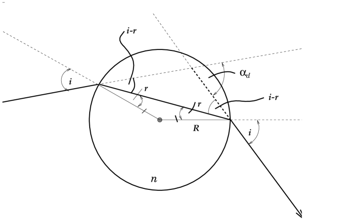
In the Fig. 4.2 we present the geometry of G-ball as a lens. From this figure and Snell’s law the deflection angle $\alpha_{\rm d}$ is

$$\alpha_{\rm d}=2\left[i-\sin^{-1}\left(\frac{1}{n}\sin i\right)\right]\,\,.$$ (4.60)

Since we consider all angles to be small, the following approximations are valid. Defining the quantity $\theta_{\rm C}=R_{\rm ball}/D_{\rm L}$, which is the radius of the region inside which the refraction occurs, we obtain the the expression for the deflection angle $\alpha_{\rm d}$

$$\alpha_{\rm d}=2\left[\sin^{-1}\left(\frac{\theta}{\theta_{\rm C}}\right)-\sin^{-1}\left(\frac{\theta}{n\theta_{\rm C}}\right)\right]\,\,.$$ (4.61)

Thus, we obtain the lens equation for the gravity ball

$$\left\{\begin{array}[]{lll}\boldsymbol{\beta}&=&\boldsymbol{\theta}-\frac{2D_{\rm LS}}{D_{\rm S}}\frac{\boldsymbol{\theta}}{\theta}\left\{\sin^{-1}\left(\frac{\theta}{\theta_{\rm C}}\right)-\sin^{-1}\left(\frac{\theta}{n\theta_{\rm C}}\right)\right\}\\ \boldsymbol{\beta}&=&\boldsymbol{\theta}\end{array}\right.\begin{array}[]{l}\mbox{for $0\leq\theta\leq\theta_{\rm C}$}\,;\\ \mbox{for $\theta>\theta_{\rm C}$}\,\,.\end{array}$$ (4.62)

where $\theta\equiv|\boldsymbol{\theta}|=\sqrt{\theta_{1}^{2}+\theta_{2}^{2}}$ is the radial position of the image in the lens plane.

Multiple image diagram and conditions for multiple imaging.

To illustrate the lensing properties described by equation (4.62) we show in Figure 4.3 the lensing curve for the gravity ball with parameters $n=1.0005$, $\theta_{\rm C}=5^{\prime}$ and for $z_{\rm source}=1$, $z_{\rm lens}=0.3$. The intersections of the lines $\beta=const$ with the curve given by equation (4.62) give the solutions to the lensing equation. The source at $\beta_{2}$ lies on a caustic point and $\theta_{\rm r}$ is the radius of the radial critical curve. The source at $\beta_{1}$ has three images, a point $\beta=0$ produces a ring—‘Einstein ring’— with the critical radius $\theta=\theta_{\rm t}$ and an image at $\theta=0$. The function $\beta(\theta)$ is continuous except at $\theta_{\rm C}$ due to the edge of the ball.

Figure 4.3: Solution to the lensing equation by a gravity ball. The solid curve represents the lensing equation curve with $n=1.0005$, $\theta_{\rm C}=5^{\prime}$, $z_{\rm source}=1$, $z_{\rm lens}=0.3$, together with lines $\beta=\beta_{i}$ (dashed lines) for various source positions $\beta_{i}$. The intersections of the lines $\beta=const$ with the lensing equation curve give the number and positions of the lensed images. The source at $\beta_{2}$ lies on a caustic point and $\theta_{\rm r}$ is the radius of the radial critical curve; source at $\beta_{1}$ has three images and point $\beta=0$ produces a ring $\theta_{\rm C}=\theta_{\rm t}$; in addition, it has an image at $\theta=0$. The function $\beta(\theta)$ is continuos except at $\theta_{\rm C}$ due to the edge of the ball.

Putting $\beta=0$ in (4.62) gives

$$\theta-\frac{2D_{\rm LS}}{D_{\rm S}}\left(\sin^{-1}{\frac{\theta}{\theta_{\rm C}}}-\sin^{-1}{\frac{\theta}{n\theta_{\rm C}}}\right)=0\,\,.$$ (4.63)

Denoting $a=2D_{\rm LS}/D_{\rm S}$, we obtain

$$\theta=a\left(\sin^{-1}\frac{\theta}{\theta_{\rm C}}-\sin^{-1}{\frac{\theta}{n\theta_{\rm C}}}\right)\,\,.$$ (4.64)

When the alignment of the source, lens and the observer is not perfect, we see features called arcs, which are the result of very strong distortion of a background sources. Arcs roughly trace the Einstein ring, so $\theta_{\rm arc}\approx\theta_{\rm E}$. Since the radii of most known arcs do not exceed $30^{\prime\prime}$ small angle approximation is valid and we obtain

$$\theta\left\{1-\frac{a}{\theta_{\rm C}}\sqrt{1-\left(\frac{\theta}{n\theta_{\rm C}}\right)^{2}}+\frac{a}{n\theta_{\rm C}}\sqrt{1-\left(\frac{\theta}{\theta_{\rm C}}\right)^{2}}\right\}=0\,\,.$$ (4.65)

One solution to this equation is trivial:

$$\theta=0\,\,,$$ (4.66)

which corresponds to the image located at the centre of the lens. To find other solutions we write the expression in the curly brackets in (4.65) as

$$\theta=\theta_{\rm C}\sqrt{1-\frac{a^{2}n^{2}}{4\theta_{\rm C}^{2}}\left(1-\frac{\theta_{\rm C}^{2}}{a^{2}}-\frac{1}{n^{2}}\right)^{2}}\,\,,$$ (4.67)

and in order to find the conditions for the Einstein ring we rewrite it in the form

$$\theta_{\rm E}=\theta_{\rm C}\sqrt{1-\frac{a^{2}n^{2}}{4\theta_{\rm C}^{2}}\left(1-\frac{\theta_{\rm C}^{2}}{a^{2}}-\frac{1}{n^{2}}\right)^{2}}\,\,.$$ (4.68)

Assuming for simplicity $a=1$ (the ball (lens) half-way between the observer and the source) and using $n$ from other estimates [107] to be from $1.001$ to $1.0001$ we obtain
for $n=1.0001$

$$\theta_{\rm E}\cong 0.98\,\theta_{\rm C}\;,$$

for $n=1.001$

$$\theta_{\rm E}\cong 0.73\,\theta_{\rm C}\,.$$

Here $\theta_{\rm E}$ is non-trivial solution of the equation (4.65). This leads to the appearence of the image in the form of a ring with the radial size of $\sim 0.9$ to $0.7$ of the total size of the ball, depending on $n$. To find the condition for the appearence of multiple images we analyze (4.67). To obtain a physical solution we take

$$1-\frac{a^{2}n^{2}}{4\theta_{\rm C}^{2}}\left(1-\frac{\theta_{\rm C}^{2}}{a}-\frac{1}{n^{2}}\right)^{2}>0\,\,.$$ (4.69)

The conditions for multiple imaging are

$$R_{\rm ball}>2D_{\rm eff}\left(1-\frac{1}{n}\right)\,\,,$$ (4.70)

or expressed through $n$

$$1<n<\frac{2D_{\rm eff}}{2D_{\rm eff}-R_{\rm ball}}\,\,,$$ (4.71)

where $D_{\rm eff}=D_{\rm LS}D_{\rm L}/D_{\rm S}$ is the effective distance.

Magnification and critical curves.

From lens equation for a G-ball (4.62) and equation (4.58) we obtain expression for the total magnification of the images

$$\mu^{-1}=\left\{1-\frac{a}{\theta}\left[\sin^{-1}\left(\frac{\theta}{\theta_{\rm C}}\right)-\sin^{-1}\left(\frac{\theta}{n\,\theta_{\rm C}}\right)\right]\right\}\times\left\{1-a\left(\frac{1}{\sqrt{\theta_{\rm C}^{2}-\theta^{2}}}-\frac{1}{\sqrt{n^{2}\theta_{\rm C}^{2}-\theta^{2}}}\right)\right\}\,\,,$$ (4.72)

where the first term represents $\mu_{\rm t}$ and second term—$\mu_{\rm r}$. In Figure 4.4 we have plotted tangential magnification $\mu_{\rm t}$ and radial magnification $\mu_{\rm r}$ against $\theta$ for a G-ball with refraction index $n=1.0006$. Singularities in these give the angular positions of tangential critical curves and radial critical curves, respectively. In the same Figure we have also plotted total magnification $\mu$ vs. $\theta$.

Figure 4.4: The magnifications: tangential $\mu_{\rm t}$ denoted by green, radial $\mu_{\rm r}$ denoted by red, and total $\mu$ is shown by blue line. Curves are plotted as a function of the image positions $\theta$ for the parameters of the lens: $n=1.0006$, $\theta_{\rm C}=5^{\prime}$, $z_{\rm l}=0.3$, $z_{\rm s}=1$. The singularities of $\mu_{\rm r}$ and $\mu_{\rm t}$ give positions of the tangential and radial critical curves, respectively.

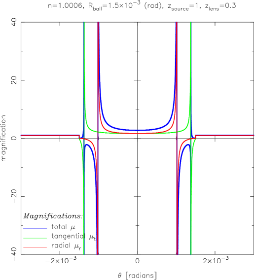
Limits on $n$ from observations.

We can rewrite equation (4.68) in terms of variables $R_{\rm ball}$ and $R_{\rm E}$ to get an expression for $R_{\rm ball}$ in terms of $n$ and a given $R_{\rm E}$.

$$R_{ball}^{2}=4D_{\rm eff}\left[1+\frac{1}{n^{2}}-\frac{\sqrt{4D_{\rm eff}^{2}-R_{\rm E}^{2}}}{nD_{\rm eff}}\right]\,\,.$$ (4.73)

Since $R_{\rm ball}\geq R_{\rm E}$, we get a lower bound on the value of $R_{\rm ball}$ if we know the radius of the Einstein ring. It is clear from the above equation that if the size of the G-ball is big enough then a large enough $n$ can give us any desired radius for the Einstein ring. If we assume that all G-balls to be of the same size, then from observations we can infer a lower bound on the radius and the refractive index inside a ball by the following argument. The radius of any gravity ball has to be larger then the radius of the largest observable Einstein ring. Given this size of the ball the refractive index should be large enough to give a real Einstein ring for every other case. This situation is illustrated in the Figure 4.5, where observational data for several clusters with giant arcs (details are presented in the Table B.1, App. B) are used with the assumption that the raduis of the arc $\theta_{\rm arc}\approx\theta_{\rm E}$. Together with the curve (4.73) for the cluster A370, we plotted the value of the radius $R_{\rm arc}$ of the A5 arc in that cluster (horizontal line), which is the largest amongst the clusters considered. It is clear that the refractive index should be greater than the value where this line intersects the $R_{\rm ball}$–$n$ curve for this cluster. Assuming all radii to be the same, we can see that in order to have an arc, a gravity ball must have $n$ more than $n\approx 1.00056$. Thus, we obtained a lower limit on $n$. Of course, our present calculations are for the case of an empty gravity ball. Matter concentrations in the centre of the ball will increase the deflection angle.

Figure 4.5: $R_{\rm ball}$ vs. $n$ for different clusters. Clusters are marked by different colours. Corresponding curves have the same colour as the name of the cluster. Details are presented in Table B.1 (App. B). Horizontal line is the value of radius of the arc A5 in the cluster A370.

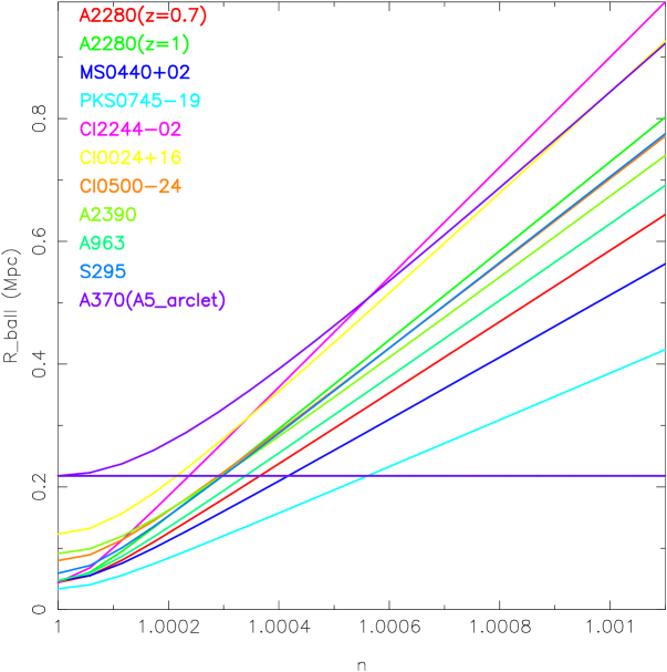
4.3.3 Simulations results

Figure 4.6: Illustration of six different images connnfigurations for an empty gravity ball. $z_{\rm l}=0.3$, $z_{\rm s}=1$, $\theta_{\rm C}=5^{\prime}$. Depending on the source position and $n$ the lens produces images of (a) ring, (b) single arc, (c) arc and opposite image, (d) radial arc, (e) three images (with two opposite arcs), (f) two images on one side (with a straight arc). Small dot in the centers of the panels marks the center of the G-ball. Small star marks the position of the source.

Figure 4.7: Distortion field generated by a simulated gravity ball. The left panel shows the grid of randomly distributed background sources as it would be seen in the absence of the lens. The middle panel shows the same population once they are distorted by a foreground gravity ball with the parameters: $z_{\rm s}=1$, $z_{\rm l}=0.3$, $\theta_{\rm C}=5^{\prime}$ rad, $n=1.001$. The right panel shows the same population distorted by a foreground (invisible) circular cluster ($z_{\rm s}=1.3$, $z_{\rm l}=0.4$, $\sigma=1000$ $kms^{-1}$); the units for both axis are in arcsecs.

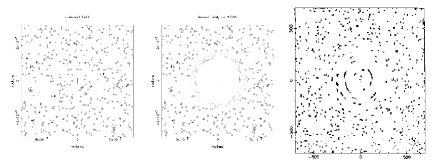
To demonstrate how a G-ball at intermediate redshift gravitationally distorts background sources we performed computer simulations and present the results in Figures 4.6 and 4.7. We have simulated an empty gravity ball the size of a typical galaxy cluster at the reshift of $z_{\rm l}=0.3$, assuming for simplicity that all source galaxies are at the same redshift $z_{\rm s}=1$. The luminous area of each background galaxy is taken to be a circular disk of radius $R$ with constant brightness. In all our numerical computations we used dimensionless Hubble parameter $h=1$. For the simulations of G-ball lensing we use the algorithm described in [73]. The image configurations by a simulated gravity ball are illustrated in Fig. 4.6 by changing the relative positions between the extended circular source and the lens. When the alignment of the source on the optical axis is perfect, the ring image—Einstein ring—appears (Fig. 4.6(a)). With a small displacement we see two opposite arcs approximately located at the Einstein radius (Fig. 4.6(e)). When the displacement becomes larger different features may appear: single tangential arc (Fig. 4.6(b)), radial arc (Fig. 4.6(d)), two opposite images (Fig. 4.6(c)) and straight arc (Fig. 4.6(f)). Figure 4.7 displays the distortion the gravity ball produces on the field of randomly distributed background sources. Figure 4.7(a) shows an unperturbed galaxy backgound projected randomly in a field of $\sim 10^{\prime}\times 10^{\prime}$ at a redshift of $z=1$. Fig. 4.7(b) illustrates the same field with an empty G-ball at the centre. To compare with the lensing effect a cluster modelled as a singular isothermal sphere produces on the background galaxies, we presented in the Fig. 4.7(c) the simulation taken from [21]. We can see from the figures that an empty gravity ball can indeed act as a strong lens and produce the images of arcs and arclets.

4.3.4 Concluding remarks

In this section we have discussed a special kind of nontopological soliton, known as gravity ball, and examined the possibility for it to be a gravitational lens. We investigated its lensing properties, calculated the deflection angle of a point source, derived the lens equation and plotted the lens curve for the gravity ball with specific parameters. We have shown that depending on the parameters of the model there can be one, two or three images (two inside the Einstein radius and one outside). However, the G-ball gravitational lens has interesting features which are not shared by other known gravitational lenses. In the case of a source, lens and observer located on the optical axis together with the Einstein ring there is always an image in the centre. Besides, the lensing geometry is radically different—there is no effect outside the lens and thus, the Einstein radius is always less than radius of the ball. The refractive index of the gravity ball contributes to the decrease in the radius of the Einstein ring and increase of its thickness. For the extended sources we showed how a large gravity ball can induce surprisingly large distortions of images of distant galaxies. It is assumed that in order to produce large arcs the cluster must have its surface-mass density approximately supercritical, $\Sigma\geq\Sigma_{crit}$. We found that the empty balls alone are able to produce arc-like features, including straight arcs, arclets and radial arcs. We have modelled the gravitational lensing effect of our gravity ball on a background source field and found that the ball produces distortion (‘shear’) of that field, consistent to some extent with the observations. We also obtained constraints on the size of the large gravity ball, which can be inferred from the existing observations of clusters with arcs. Empty G-balls can show in observations as arcs without evident mass distribution—a lens and/or through the distortion of the background random galaxy field.

Observationally empty G-balls have not yet been found, but we conclude from our analysis that the existence of large G-balls cannot be ruled out by gravitational lensing effects.

Chapter 5 Propagation of Light in Strong Gravitational Fields

5.1 Introduction and main motivations

As described in the Introduction to the thesis (2.1), gravitational lensing in strong gravitational fields leads to many astrophysically interesting effects. In this section we discuss yet another one.

The idea that centres of the globular clusters host massive (up to $10^{4}\,M_{\odot}$) black holes (BH) goes back to 1975, when scientists were trying to detect them through X-ray emission. Since then other methods were proposed. In particular, the observations of the millisecond (ms) pulsars in globular clusters can help, since the pulsar motion would be governed by the presence of massive black hole in the centre of the globular cluster ([125],[121] and references within). A large number of ms pulsars have been discovered in globular clusters—more than 35 ms and 4 long-period ones in 13 Galactic globular clusters have been reported. This is not surprising, since the dense stellar field in the globular clusters provides a favourable environment for frequent stellar encounters to form low-mass-X-ray-binaries (LMXB). These are believed to be the progenitors of the ms pulsars. By some estimates (for ex. [118]), the total number of pulsars in Galactic globular clusters, beaming at us, most likely lies between 300 and 2000. This provides an excellent opportunity to use them for revealing the existence of central black holes. A possible mechanism for establishing the presence of massive black hole in the centre, which has not so far attracted any attention, is through the gravitational lensing of the pulsar’s radiation by the central mass. It is only logical to suppose that the black hole in the centre of the globular cluster would be a rotating black hole. There exist a number of papers investigating the lensing properties of Kerr black holes. Bray [119] was the first to investigate the properties of the isolated Kerr black hole as a gravitational lens. He demonstrated that effect of spin of the BH comes in the second order terms of the expansion of null geodesics in the Kerr metric and considered the conditions for the multiple imaging. Simulteneously, Dymnikova [122] studied the time dilation, in the sense of Shapiro effect, and showed how the asymmetry in the time delay depends on the mutual orientation of a photon propagation direction and of the rotation axis. The photon is accelerated, if its motion is along the direction of the rotation, and it is delayed otherwise [124]. This effect can be traced back to the dragging of inertial frames. The asymmetry’s is very enhanced in the regions corresponding to lensing and increases sharply for the photons traveling very close to the central body. If, for example, the motion is retrograde, the effect of the rotation is to impose an additional time delay acting in the same direction as the effect arising from the mass. For systems with the central rotating black hole the time lag can be of the order of minutes [123].

One more interesting effect was noted by Carini et al [120]. They showed that angular momentum of a Kerr black hole gives rise to a rotation of the plane of polarization of a linearly polarized light. They noted that the rotation of the polarization plane induced by the angular momentum of the central gravitational source is analogous to Faraday effect of the electromagnetic wave propagating through magnetized plasma and thus may be referred to as the "gravitational Faraday rotation".

Still more effects may also possibly exist—in particular, it may be interesting to study the differential frequency shift between the beams propagating in the equatorial plane (where this effect would be maximal) on the opposite sides of the black hole. Secondly, for a source of pulsed radiation (e.g. pulsars), it would be interesting to determine if a mechanism exists which can produce the difference in the time period between pulses in two images. In that case it could be possible that some (?) of the pulsars in certain globular clusters are gravitationally lensed images of the same source. This is the main motivation with which the present work has started.

5.2 Photons in a gravitational field

It was Galileo’s famous experiment that asserted that big balls fall at the same rate as small balls. By the more general statement, known as EP (Einstein equivalence principle) all particles follow the same geodesic path, independent of the mass or internal structure. Photons move along null geodesics in curved spacetime, and all photons are deflected in a gravitational potential by the same angle independent of their energy or polarization. This is mostly used in studies of the gravitational lensing around black holes. However, some special situations are reported, where gravitational birefringence and dispersive effects are described. For example, in quantum electrodynamics, virtual electron loops induce curvature couplings in the effective action of low-frequency photons [126]. In such a case, photon propagation can be influenced by tidal effects coming from local spacetime curvature. Drummonds and Hathrell [127] found that the propagation of photons in spatially anisotropic background (Schwarzchild and gravitational-wave) was polarization-dependent. Similarly, gravitational birefringence was also found to occur in Reissner-Norström spacetimes [128]. The energy-dependent deflection of light was shown in the context of string theory [130] and higher derivative gravity, which arises from QED radiative corrections [126]. There is some controversy in literature. For example, Masshoon firmly states that birefringence is possible only if the central body is a rotating body and it is a consequence of the coupling of the intrinsic spin of the photon with the rotation of the central body. That is, for a Schwarzschild black hole the amplitudes for the scattering of right circular polarized (RCP) and left circular polarized (LCP) waves are equal and, hence, the spherical symmetry of this field preserves the polarization of the incident radiation in the scattered waves. However, for a Kerr black hole RCP and LCP radiations are scattered differently and the deflection of the radiation by a rotating mass becomes polarization dependent [131].

5.2.1 Spinning particles

We would like to pay special attention here to the fact that photon is an elementary particle with spin. Spin angular momentum of matter, occurring in nature in units of ${\raise-0.15pt\hbox{$\mkern-0.5mu\barbar$}\mkern-8.5muh}/2$, is the physical notion which seems necessary for a successful extension of GR to microphysics. All elementary particles can be classified by means of irreducible unitary representations of the Poincarè group and can be labeled by mass $m$ and spin $s$. Mass is connected with the translational part of the Poincarè group and spin with the rotational part. Mass and spin are elementary notions, each with an analogous standing not reducible to that of the other.

The problem of the motion of a particle with internal angular momentum (spin) in external gravitational field consists of two parts: spin precession and spin influence on the trajectory of motion. Gyroscope precession in a centrally symmetric gravitational field was considered more than 70 years ago [132] and is now a well-described effect, since it is extremely important in the satellite industry. The situation is different with the second part of the problem, which refers to the spin influence on the trajectory. According to EP a spinning mass should fall at the same rate as non-spinning one. However, in a seminal paper, Papapetrou [133] showed that trajectories of spinning particles (in the limit of a vanishing mass) deviate from geodesics. His derivation was based upon taking a macroscopic mass, expanding it in moments about the center, and deriving the equations of motion for each moment. The basic result was that the deviation is proportional to the spin of the particle (vanishing for a zero spin) and the curvature of the space. It is presumed that the results are valid for fundamental particles, but there is no classical theory that yields the result [134]. The difficulty is that there has not been a satisfactory theory which derives these equations from a variational principle. There have been numerous attempts, though; a good review on equations for particles with spin is recently presented by Frydryszak [135]. Most recent claims, involving a generalized Clifford algebras, are presented by Pezzaglia [136]. The problem of the influence of spin on the trajectory of a particle in an external gravitational field is not merely of a theoretical interest. This problem is closely related to the gravitational waves field, where one has to calculate the gravitational waves radiation from the inspiralling black (Kerr) holes. In gravitational lensing this problem can be of the importance. It could lead to the deviation of the photon trajectories from the geodesics and to the gravitational birefringence in an arbitrary gravitational field. In the next section, the modified geodesic equations of photon in an external gravitational field are investigated. The results obtained in the Section 5.3 are used in the subsequent section (Section 5.4) in the context of recent claims [127, 128, 137] that photons acquire superluminal velocities in the Schwarzschild , FRW and gravitational wave background. We extend the results obtained by [138] to the Kerr background and find, in concordance to previous results for other metrics, that in Kerr metric this does not happen. In the last section we derive the Papapetrou equations for the photon directly.

5.3 Modified geodesic equation for photons

5.3.1 Theoretical background

The action of the electromagnetic field in the curved spacetime is given by:

$$S=\int\,d^{4}x\,\sqrt{-g}F_{\mu\nu}F^{\mu\nu},$$ (5.1)

where $F_{\mu\nu}$ has its usual meaning$F_{\mu\nu}=A_{\mu;\nu}-A_{\nu;\mu}$. Varying the action with respect to $A_{\mu}$ we obtain the source equations for a free electromagnetic field in curved space-time:

$$\nabla^{\nu}F_{\mu\nu}=0\,\,.$$ (5.2)

These equations together with the property of the field:

$$\nabla_{[\mu}F_{\lambda\nu]}=0$$ (5.3)

constitute Maxwell equations in an empty 4-space. To obtain a wave equation for a photon, we will apply $\nabla^{\mu}$ to the Eq. 5.3:

$$\nabla^{\mu}\left(\nabla_{\mu}F_{\nu\lambda}\right)+\nabla^{\mu}\left(\nabla_{\nu}F_{\lambda\mu}\right)+\nabla^{\mu}\left(\nabla_{\lambda}F_{\mu\nu}\right)=0\,\,.$$ (5.4)

Using the properties of a commutator of the covariant derivatives

$$\left[\nabla^{m},\nabla_{n}\right]A_{ik}=\nabla^{m}\left(\nabla_{n}A_{ik}\right)-\nabla_{m}\left(\nabla_{n}A_{ik}\right)\,\,,$$

and from the field equations (5.3) we have

$$\square F_{\nu\lambda}+\underbrace{\left[\nabla^{\mu},\nabla_{\nu}\right]F_{\lambda\mu}}_{\mbox{\char 172}}+\underbrace{\left[\nabla^{\mu},\nabla_{\lambda}\right]F_{\mu\nu}}_{\mbox{\char 173}}=0\,\,.$$ (5.5)

The operator $\square$ will be frequently referred to. In general coordinates it is to be taken as defined by

$$\square A_{\mu\nu...}\stackrel{{\scriptstyle\mathrm{def}}}{{\equiv}}g^{\alpha\beta}\left(A_{\mu\nu...}\right)_{;\alpha;\beta}$$ (5.6)

It is also sometimes written in the form (see [139], p. 64) $\square=\left(\left(...\right)_{;\alpha}\right)^{;\alpha}$, that is, we perform a covariant and a contravariant differentiation and contract them. In some texts it means also $\square=\nabla^{\mu}\nabla_{\mu}$, where $\nabla$ is a covariant derivative.
Following the definition of a commutator of covariant derivatives

$$\left[\nabla_{c},\nabla_{d}\right]X^{a}_{\;\;b}\stackrel{{\scriptstyle\mathrm{def}}}{{=}}R^{a}_{\;\;\lambda cd}X^{\lambda}_{\;\;b}-R^{\lambda}_{\;\;bcd}X^{a}_{\;\;\lambda}\,\,,$$ (5.7)

we expand the numbered terms in the equation (5.5):

① $$\left[\nabla^{\mu},\nabla_{\nu}\right]F_{\lambda\mu}\equiv\left[\nabla_{\mu},\nabla_{\nu}\right]F_{\lambda}^{\;\;\mu}=-\left[\nabla_{\mu},\nabla_{\nu}\right]F^{\mu}_{\;\;\lambda}=R^{\rho}_{\;\;\lambda\mu\nu}F^{\mu}_{\;\;\rho}-\hskip 289.07999pt$$

$$-R^{\mu}_{\;\;\rho\mu\nu}F^{\rho}_{\;\;\lambda}=R^{\rho}_{\;\;\lambda\mu\nu}F^{\mu}_{\;\;\rho}-R_{\rho\nu}F^{\rho}_{\;\;\lambda}\,\,.$$

② $$\left[\nabla^{\mu},\nabla_{\lambda}\right]F_{\mu\nu}\equiv\left[\nabla_{\mu},\nabla_{\lambda}\right]F^{\mu}_{\;\;\nu}=R^{\mu}_{\;\;\rho\mu\lambda}F^{\rho}_{\;\;\nu}-R^{\rho}_{\;\;\nu\mu\lambda}F^{\mu}_{\;\;\rho}=\hskip 722.7pt$$

$$=R_{\rho\lambda}F^{\rho}_{\;\;\nu}-R^{\rho}_{\;\;\nu\mu\lambda}F^{\mu}_{\;\;\rho}\,\,.$$

Using symmetry properties of a Riemann tensor

$$R^{\rho}_{\;\;\lambda\mu\nu}=-R^{\rho}_{\;\;\lambda\nu\mu}\stackrel{{\scriptstyle\&}}{{\Longrightarrow}}R^{\rho}_{\;\;\nu\mu\lambda}=-R^{\rho}_{\;\;\lambda\nu\mu}-R^{\rho}_{\;\;\mu\lambda\nu}$$

we obtain the wave equation for a photon in a curved space-time:

$$\square F_{\nu\lambda}-R_{\rho\nu}F^{\rho}_{\;\;\lambda}+R_{\rho\lambda}F^{\rho}_{\;\;\nu}+R^{\rho}_{\;\;\mu\lambda\nu}F^{\mu}_{\;\;\rho}=0\,\,.$$ (5.8)

In empty space this equation becomes

$$\square F_{\nu\lambda}+R^{\rho}_{\;\;\mu\lambda\nu}F^{\mu}_{\;\;\rho}=0\,\,.$$ (5.9)

This equation was first derived by Eddington [139], though not from the action. This equation is quite unusual, therefore it deserves some more explanations. Let us consider the 4-potential $A_{\mu}$. Since it is not gauge invariant, we will add the standard Lorentz gauge:

$$\left(A^{\mu}\right)_{;\mu}=0\,\,.$$ (5.10)

With the boundary condition at the infinity, the value of $A_{\mu}$ becomes completely determined.

From Maxwell equations in the presence of a source, we get

$$J^{\mu} = \left(F^{\mu\nu}\right)_{;\nu}=\left(g^{\alpha\beta}F_{\mu\beta}\right)_{;\alpha}=g^{\alpha\beta}\left(F_{\mu\beta}\right)_{;\alpha}=g^{\alpha\beta}\left(A_{\mu;\beta;\alpha}-A_{\beta;\mu;\alpha}\right)=$$

$$g^{\alpha\beta}\left(A_{\mu;\beta;\alpha}-A_{\beta;\alpha;\mu}+R^{\epsilon}_{\;\;\beta\alpha\mu}A_{\epsilon}\right)=g^{\alpha\beta}\left(A_{\mu}\right)_{;\beta;\alpha}-\left(A^{\alpha}_{;\alpha}\right)_{;\mu}+R^{\epsilon}_{\;\mu}A_{\epsilon}\,\,.$$

In the Lorentz gauge, we have

$$\square A_{\mu}=J_{\mu}-R^{\epsilon}_{\mu}A_{\epsilon}\,\,.$$

In empty space this becomes $\square A_{\mu}=0$, showing that $A_{\mu}$ is propagated with the fundamental velocity. We see that the velocity of propagation of electromagnetic potential and of electromagnetic force is not the same. It should not be surprising, since $A_{\mu}$ is not physically important, being fixed by arbitraty convention (Eq. 5.10). Bu the result (5.8) is very interesting, showing that Ricci and Riemann curvature coupling terms give rise to the polarization dependent deviation of photon orbits from null geodesics. The derivation of the result (5.8) from the action principle was first given in [138].

In order to derive equation for the characteristics of photon propagation we make the geometrical optics plane-wave approximation. In geometrical optics, one assumes that the electromagnetic waves have a wavelength which is much smaller than the radius of curvature of the background geometry, or the scale of variation of the amplitude of the wave front. We also assume in our analysis that the influence of the electromagnetic field on the metric field can be neglected. Thus, “locally plane" waves can be represented by approximate solutions of Maxwell’s equations of the form

$$F_{\mu\nu}=e^{is(x)}f_{\mu\nu}\,\,,$$ (5.11)

where $f_{\mu\nu}$ is a lowly varying amplitude, and $s$, a rapidly oscillating phase. (It is understood that one takes the real part of the right hand side of Eq. 5.11). We should emphasize that although this is an approximation for the actual solution for the photon, it exactly determines the characteristics of propagation and hence the casual structure of the solution, at least in domains where the gradient of the $s$ does not vanish [14]. The wave vector $k_{\mu}$ is given by the gradient of the phase

$$k_{\mu}=\nabla_{\mu}s\,\,.$$ (5.12)

Operating by $\nabla_{\mu}$ on (5.11) and neglecting the derivative of a slow changing amplitude, we obtain

$$\nabla_{\mu}F_{\alpha\beta}=i\,F_{\alpha\beta}\nabla_{\mu}\,s=ik_{\mu}F_{\alpha\beta}\,\,.$$ (5.13)

Using (5.11), Eq. 5.8 becomes

$$\nabla^{\mu}\nabla_{\mu}\left(e^{is}f_{\nu\lambda}\right)-R^{\rho}_{\;\nu}F_{\rho\lambda}+R^{\rho}_{\;\lambda}F_{\rho\nu}+R^{\rho\mu}_{\;\;\;\;\lambda\nu}F_{\mu\rho}=0\,\,.$$

Considering $k_{\mu}$ a constant vector, after some algebra we obtain the wave equation (5.8) gives

$$-k_{\mu}k^{\mu}f_{\nu\lambda}+R^{\rho}_{\;\lambda}f_{\rho\nu}+R^{\rho\mu}_{\;\;\;\;\lambda\nu}f_{\mu\rho}-R^{\rho}_{\;\nu}f_{\rho\lambda}=0\,\,.$$ (5.14)

Since, by definition, wave vector $k_{\mu}$ is a gradient, $\nabla^{\alpha}k_{\mu}=\nabla_{\mu}k^{\alpha}$, and

$$\nabla^{\alpha}\left(k_{\mu}k^{\mu}\right)=2k^{\mu}\nabla_{\mu}k^{\alpha}\,\,.$$

Light rays are defined as the integral curves $x^{\alpha}(s)$ of the vector field $k^{\alpha}$, that is, $k^{\alpha}=dx^{\alpha}/ds$. Therefore,

$$\nabla^{\alpha}\left(k^{\mu}k_{\mu}\right)=2\frac{dx^{\mu}}{ds}\left(k^{\alpha}\right)_{;\mu}=2\frac{dx^{\mu}}{ds}\left(k^{\alpha}_{\;\;,\mu}+\Gamma^{\alpha}_{\;\;\mu\sigma}k^{\sigma}\right)=$$ (5.15)

$$= 2\frac{dx^{\mu}}{ds}\left(\frac{\partial}{\partial x^{\mu}}\frac{dx^{\alpha}}{ds}+\Gamma^{\alpha}_{\;\;\mu\sigma}\frac{dx^{\sigma}}{ds}\right)=2\left(\frac{d^{2}x^{\alpha}}{ds^{2}}+\Gamma^{\alpha}_{\;\;\mu\sigma}\frac{dx^{\mu}}{ds}\frac{dx^{\sigma}}{ds}\right)\,\,.$$

We can write the Eq. 5.14 in the form:

$$k^{2}f_{\nu\lambda}=R^{\rho}_{\;\lambda}f_{\rho\nu}+R^{\rho\mu}_{\;\;\;\;\lambda\nu}f_{\mu\rho}-R^{\rho}_{\;\nu}f_{\rho\lambda}\,\,,$$

and obtain the dispersion relation for the wave vector:

$$k^{2}=\left(R^{\rho\mu}_{\;\;\;\;\lambda\nu}f_{\mu\rho}+R^{\rho}_{\;\lambda}f_{\rho\nu}-R^{\rho}_{\;\nu}f_{\rho\lambda}\right)\cdot\frac{f^{\nu\lambda}}{(f_{\alpha\beta}f^{\alpha\beta})}\,\,.$$ (5.16)

Combining (5.15) and (5.16), we obtain the modified geodesic equation for photons:

$$\frac{d^{2}x^{\alpha}}{ds^{2}}+\Gamma^{\alpha}_{\mu\sigma}\frac{dx^{\mu}}{ds}\frac{dx^{\sigma}}{ds}=\frac{1}{2}\nabla^{\alpha}\left[\left(R^{\rho\mu}_{\;\;\;\;\lambda\nu}f_{\mu\rho}+R^{\rho}_{\;\lambda}f_{\rho\nu}-R^{\rho}_{\;\nu}f_{\rho\lambda}\right)\frac{f^{\nu\lambda}}{(f_{\alpha\beta}f^{\alpha\beta})}\right]\,\,.$$ (5.17)

The nonzero right hand side of the modified geodesic equation leads to a polarization dependance in the gravitational redshift, deflection angle and Shapiro time delay of light. In order to investigate these equations we consider the Schwarzschild  space-time.

5.3.2 Schwarzschild metric

Schwarzschild metric is represented by:

$$d\tau^{2}=\left(1-\frac{2m}{r}\right)\,dt^{2}-\left(1-\frac{2m}{r}\right)^{-1}\,dr^{2}-r^{2}\,d\theta^{2}-r^{2}\sin^{2}{\theta}\,d\phi^{2}\,\,.$$ (5.18)

Equations of motion (Eq. 5.17) in an empty space are:

$$\frac{d^{2}x^{\alpha}}{ds^{2}}+\Gamma^{\alpha}_{\mu\nu}\frac{dx^{\mu}}{ds}\frac{dx^{\nu}}{ds}=\frac{1}{2}\underbrace{\nabla^{\alpha}\left(R_{\rho\mu\nu\lambda}f^{\rho\mu}\right)}_{\circledast}\frac{f^{\nu\lambda}}{|f^{2}|}\,\,.$$ (5.19)

Covariant derivative of a Riemann tensor:

$$R_{\alpha\beta\mu\nu;\lambda}=R_{\alpha\beta\mu\nu,\lambda}-\Gamma^{k}_{\alpha\lambda}R_{k\beta\mu\nu}-\Gamma^{k}_{\beta\lambda}R_{\alpha k\mu\nu}-\Gamma^{k}_{\mu\lambda}R_{\alpha\beta k\mu}-\Gamma^{k}_{\nu\lambda}R_{\alpha\beta\mu k}\,\,.$$ (5.20)

After expanding $\circledast$, the right hand side of the Eq. 5.19 is:

$$\mbox{R.H.S.}=\frac{1}{2|f^{2}|}\left[f^{\rho\mu}\left(\partial_{\alpha}R_{\rho\mu\nu\lambda}-\Gamma^{k}_{\rho\alpha}R_{k\mu\nu\lambda}-\Gamma^{k}_{\mu\alpha}R_{\rho k\nu\lambda}-\Gamma^{k}_{\;\;\nu\alpha}R_{\rho\mu k\lambda}-\right.\right.$$

$$-\left.\left.\Gamma^{k}_{\lambda\alpha}R_{\rho\mu\nu k}\right)+R_{\rho\mu\nu\lambda}\left(\partial_{\alpha}f^{\rho\mu}+\Gamma^{\rho}_{\alpha k}f^{k\mu}+\Gamma^{\mu}_{\alpha k}f^{\rho k}\right)\right]f^{\nu\lambda}\,\,.$$ (5.21)

We will write this equation in components.

A.

Let $\alpha=\varphi$.
Due to the axisymmetry of the metric,

$$\partial_{\varphi}R_{\rho\mu\nu\lambda}=0\,\,,$$

$$\partial_{\varphi}f^{\rho\mu}=0\,\,.$$

After expanding $\nabla^{\varphi}$, the right hand side (Eq. 5.21) is:

$$\mbox{RHS}=\frac{2}{|f^{2}|}\left[f^{tr}f^{t\varphi}\,\Gamma^{\varphi}_{r\varphi}R_{t\varphi t\varphi}+f^{t\theta}f^{t\varphi}\,\Gamma^{\varphi}_{\theta\varphi}R_{t\varphi t\varphi}+f^{tr}f^{t\varphi}\,\Gamma^{r}_{\varphi\varphi}R_{trtr}+f^{t\varphi}f^{t\theta}\,\Gamma^{\theta}_{\varphi\varphi}R_{t\theta t\theta}\right]\,\,.$$

Using the non-vanishing components of the affine connection and Riemann tensor, we find:

$$\mbox{RHS}=\frac{6m(2m-r)\sin^{2}{\theta}}{r^{3}}\frac{f^{tr}f^{t\varphi}}{f^{2}}\,\,.$$

B.

$\alpha=t$

$$\partial_{t}R_{\rho\mu\nu\lambda}=0\,\,,$$

and we use the fact that in the absence of charges $\partial_{\alpha}f^{\alpha\beta}=0$. After expanding $\nabla^{t}$, the RHS for the time component $t$ is:

$$\mbox{RHS}=0\,\,.$$

C.

$\alpha=r$
After expanding $\nabla^{r}$, the RHS for the $r$ component is:

$$\mbox{RHS}=\frac{2}{|f^{2}|}\left[\left(f^{tr}\right)^{2}\partial_{r}R_{trtr}+\left(f^{t\theta}\right)^{2}\partial_{r}R_{t\theta t\theta}+\left(f^{t\varphi}\right)^{2}\partial_{r}R_{t\varphi t\varphi}++f^{t\theta}R_{t\theta t\theta}\,\partial_{r}f^{t\theta}+\right.$$

$$+\left.f^{t\varphi}R_{t\varphi t\varphi}\,\partial_{r}f^{t\varphi}--\left(f^{t\theta}\right)^{2}R_{t\theta t\theta}\left(\Gamma^{t}_{tr}+\Gamma^{\theta}_{r\theta}\right)-\left(f^{t\varphi}\right)^{2}R_{t\varphi t\varphi}\left(\Gamma^{t}_{tr}+\Gamma^{\varphi}_{r\varphi}\right)\right]\,\,.$$

Using non-vanishing components of the affine connection and Riemann tensor, we find:

$$\mbox{RHS}=\frac{2m}{r^{2}}\frac{1}{f^{2}}\left[-\left(f^{rt}\right)^{2}\frac{6}{r^{2}}+\left(f^{\theta t}\right)^{2}\frac{(2r-5m)}{r}++\left(f^{\varphi t}\right)^{2}\frac{(2r-5m)\sin^{2}{\theta}}{r}+\right.$$

$$+\left.f^{\theta t}\,\partial_{r}f^{\theta t}\,(2m-r)+f^{\varphi t}\,\partial_{r}f^{\varphi t}\,(2m-r)\sin^{2}{\theta}\right]\,\,.$$

D.

$\alpha=\theta$
After expanding $\nabla^{\theta}$, the RHS for $\theta$ component is:

$$\mbox{RHS}=\frac{2}{|f^{2}|}\left[\left(f^{rt}\right)^{2}\partial_{\theta}R_{trtr}+\left(f^{t\theta}\right)^{2}\partial_{\theta}R_{t\theta t\theta}+\left(f^{t\varphi}\right)^{2}\partial_{\theta}R_{t\varphi t\varphi}++f^{tr}R_{trtr}\,\partial_{\theta}f^{tr}+\right.$$

$$+ \left.f^{t\varphi}R_{t\varphi t\varphi}\,\partial_{\theta}f^{t\varphi}-f^{tr}f^{t\theta}\left(\Gamma^{r}_{\theta\theta}R_{trtr}+\Gamma^{\theta}_{r\theta}R_{t\theta t\theta}\right)-\left(f^{t\varphi}\right)^{2}\Gamma^{\varphi}_{\theta\varphi}R_{t\varphi t\varphi}\right]\,\,.$$

Using non-vanishing components of the affine connection and Riemann tensor, we find:

$$\mbox{RHS}=\frac{2m}{r^{2}}\frac{1}{f^{2}}\left[\left(f^{\varphi t}\right)^{2}3(r-2m)\cos{\theta}\sin{\theta}+f^{t\theta}f^{tr}\,\frac{3(r-2m)}{r}+\right.$$

$$+\left.f^{tr}\,\partial_{\theta}f^{tr}\,\frac{2}{r}+f^{t\varphi}\,\partial_{\theta}f^{t\varphi}\,(2m-r)\sin^{2}{\theta}\right]\,\,.$$

For the equatorial plane, $\theta=\pi/2$, the equations are simplified:
RHS for $r$

$$\mbox{RHS}=\frac{2m}{r^{2}}\frac{1}{f^{2}}\left[-\left(f^{rt}\right)^{2}\frac{6}{r^{2}}+\left(f^{\theta t}\right)^{2}\frac{(2r-5m)}{r}\,+\right.$$

$$\left.\left(f^{\varphi t}\right)^{2}\frac{(2r-5m)}{r}+f^{\theta t}\,\partial_{r}f^{\theta t}(2m-r)+f^{\varphi t}\,\partial_{r}f^{\varphi t}\,(2m-r)\right]\,\,,$$

RHS for $\varphi$

$$\mbox{RHS}=\frac{6m(2m-r)}{r^{3}}\frac{f^{tr}f^{t\varphi}}{f^{2}}\,\,,$$

RHS for $\theta$:

$$\mbox{RHS}=\frac{6m(r-2m)}{r^{3}}\frac{f^{t\theta}f^{tr}}{f^{2}}\,\,,$$

RHS for $t$:

$$\mbox{RHS}=0\,\,.$$

5.3.3 The final set of equations

Combining together left hand sides and right hand sides and noticing that we considered the amplitude to be nearly constant, the equations of motion are:

Equation for $r$:

$$\frac{d^{2}r}{ds^{2}}+\frac{m(r-2m)}{r^{3}}\left(\frac{dt}{ds}\right)^{2}-\frac{m}{r(r-2m)}\left(\frac{dr}{ds}\right)^{2}-(r-2m)\left(\frac{d\theta}{ds}\right)^{2}-(r-2m)\sin^{2}{\theta}\left(\frac{d\varphi}{ds}\right)^{2}=$$

$$\frac{2m}{r^{2}}\frac{1}{|f^{2}|}\left[-\frac{6}{r^{2}}\left(f^{rt}\right)^{2}+\frac{(2r-5m)}{r}\left(f^{\theta t}\right)^{2}+\frac{(2r-5m)\sin^{2}{\theta}}{r}\left(f^{\varphi t}\right)^{2}\right]\,\,.$$ (5.22)

Equation for $\theta$:

$$\frac{d^{2}\theta}{ds^{2}}+\frac{2}{r}\frac{d\theta}{ds}\frac{dr}{ds}-\sin{\theta}\cos{\theta}\left(\frac{d\varphi}{ds}\right)^{2}=\frac{2m}{r^{2}}\frac{1}{|f^{2}|}\left[\frac{3(r-2m)}{r}f^{tr}f^{t\theta}+3(r-2m)\cos{\theta}\sin{\theta}\left(f^{t\varphi}\right)^{2}\right]\,\,.$$

Equation for $\varphi$:

$$\frac{d^{2}\varphi}{ds^{2}}+\frac{2}{r}\frac{dr}{ds}\frac{d\varphi}{ds}+2\cot{\theta}\,\frac{d\theta}{ds}\frac{d\varphi}{ds}=\frac{6m(2m-r)\sin^{2}{\theta}}{r^{3}}\frac{f^{tr}f^{t\varphi}}{|f^{2}|}\,\,.$$ (5.24)

Equation for $t$:

$$\frac{d^{2}t}{ds^{2}}+\frac{2m}{r(r-2m)}\frac{dt}{ds}\frac{dr}{ds}=0\,\,.$$ (5.25)

And for $\theta=\pi/2$, they become

$$\mbox{[a]}\hskip 14.45377pt\frac{d^{2}\varphi}{ds^{2}}+\frac{2}{r}\frac{dr}{ds}\frac{d\varphi}{ds}=\frac{6m(2m-r)}{r^{3}}\frac{f^{tr}f^{t\varphi}}{f^{2}}\,;$$

$$\mbox{[b]}\hskip 14.45377pt\frac{d^{2}t}{ds^{2}}+\frac{2m}{r(r-2m)}\frac{dt}{ds}\frac{dr}{ds}=0\,;$$

$$\mbox{[c]}\hskip 14.45377pt\frac{d^{2}\theta}{ds^{2}}=\frac{6m(r-2m)}{r^{3}}\frac{f^{t\theta}f^{tr}}{f^{2}}\,;$$

$$\begin{split}&\mbox{[d]}\hskip 14.45377pt\frac{d^{2}r}{ds^{2}}-\frac{m}{r(r-2m)}\left(\frac{dr}{ds}\right)^{2}-(r-2m)\left(\frac{d\varphi}{ds}\right)^{2}+\frac{m(r-2m)}{r^{3}}\left(\frac{dt}{ds}\right)^{2}=\\[5.05942pt] &=\frac{2m}{r^{2}}\frac{1}{f^{2}}\left[-\left(f^{rt}\right)^{2}\frac{6}{r^{2}}+\left(f^{\theta t}\right)^{2}\frac{(2r-5m)}{r}+\left(f^{\varphi t}\right)^{2}\frac{(2r-5m)}{r}\right]\,\,.\end{split}$$ (5.26)

Eqs. 5.26 give the following conserved quantity, the energy $E$:

$$\frac{r-2m}{r}\frac{dt}{ds}=E\,\,.$$ (5.27)

However, we notice from Eqs. LABEL:eq:theta and 5.24 that the direction of the angular momentum is not preserved; photon that started at, say, $\theta=\pi/2$, will not remain in the equatorial plane—the right hand side of the Eq. 5.26[c] gives the acceleration to a photon in the $\theta$ direction.

5.4 Velocity of photons in Kerr metric

In this section we come back to the results of the Section 5.3 in view of the claims [127, 137] that in higher derivative gravity which arises by QED radiative corrections, the photon velocity in local inertial frame can exceed the velocity of light in the Minkowski background. This result was extended by Daniels & Shore to charged [128] and rotating black holes [129] with the same conclusions. However, Mohanty & Prasanna [138] showed that the claims of superluminal photon velocity are due to the neglect of the curvature coupling terms in the wave equation derived from the minimal $F_{\mu\nu}F^{\mu\nu}$ Lagrangian (see Section 5.3, Eq. 5.8) and that the velocity of photons is less than $c$ in Schwarzschild and FRW metrics, as well as in a higher derivative gravity, (as long as the SEC (see Section 3.1) is satisfied). We extended these results to a Kerr gravitational background.

5.4.1 $\epsilon$-matrix

To obtain the photon velocity we will use the dispersion relation (Eq. 5.16). Due to the internal Maxwell equations (5.3), only three components of $F_{\mu\nu}$ are independent. Choosing the components of the electric field vector $E_{i}=f_{oi}$ as the independent components, we have from (5.3) and (5.13

$$k_{0}f_{ij}+k_{i}f_{j0}+k_{j}f_{0i}=0\,\,.$$ (5.28)

Using (5.28) to substitute for $f_{ij}$ in terms of electric field components $f_{j0}$ and $f_{0i}$ in the wave equation (5.14), we obtain

$$-k_{\mu}k^{\mu}f_{0i}-R^{j}_{\,\,i}f_{0j}-R^{0}_{\,\,0}f_{0i}+R^{j}_{\,\,0}\frac{k_{i}}{k_{0}}f_{0j}-R^{j}_{\,\,0}\frac{k_{j}}{k_{0}}f_{0i}+2R^{0j}_{\,\,\,\,0i}f_{0j}+4R^{lj}_{\,\,\,\,0i}\frac{k_{l}}{k_{0}}f_{0j}=0\,\,.$$ (5.29)

Rewriting it through only one component, $f_{0j}$, gives

$$\left[\left(k_{\mu}k^{\mu}+R^{0}_{\,\,0}+R^{l}_{\,\,0}\frac{k_{l}}{k_{0}}\right)\delta^{j}_{i}+\left(R^{j}_{\,\,i}-R^{j}_{\,\,0}\frac{k_{i}}{k_{0}}-2R^{0j}_{\,\,\,\,0i}-4R^{lj}_{\,\,\,\,0i}\frac{k_{l}}{k_{0}}\right)\right]f_{0j}=0\,\,.$$ (5.30)

This is the wave equation obeyed by the three components of the electric field vector. We can simplify this equation by defining the matrix $\epsilon_{i}^{\,\,j}$:

$$\epsilon_{i}^{\,\,j}\equiv\left(R^{0}_{\,\,0}+R^{l}_{\,\,0}\frac{k_{l}}{k_{0}}\right)\delta^{j}_{i}+\left(R^{j}_{\,\,i}-R^{j}_{\,\,0}\frac{k_{i}}{k_{0}}-2R^{0j}_{\,\,\,\,0i}-4R^{lj}_{\,\,\,\,0i}\frac{k_{l}}{k_{0}}\right)\,\,,$$ (5.31)

and thus, (5.30) becomes

$$\left(k^{2}\delta^{j}_{i}+\epsilon^{j}_{i}\right)f_{0j}=0\,\,.$$ (5.32)

We can rewrite this equation as matrix equation and by diagonalising the $\epsilon_{i}^{j}$, we find the equations for normal modes:

$$\epsilon_{i}^{j}f_{0j}=-k^{2}f_{0i}\,\,,$$

and

$$\left(k^{2}+\epsilon_{i}\right)f_{0i}=0\;\;\;\;(i=1,2,3)\,\,,$$ (5.33)

where $\epsilon_{i}$ are the eigenvalues of the $e_{j}^{i}$ matrix. By defining the projection operator $P_{jk}=\delta_{jk}-n_{j}n_{k}$, with $n^{i}=k^{i}/|{\bf n}|$, these equations can be decomposed into a transverse part

$$f_{0j}^{(T)}=\left(\delta_{j}^{i}-n^{i}n_{j}\right)f_{0i}\,\,,$$ (5.34)

and a longitudal part

$$f_{0j}^{(L)}=n^{i}n_{j}f_{0i}\,\,.$$ (5.35)

By substituting back into (5.33), we obtain the wave equations for the transverse photons (polarization)

$$\left[k^{2}+\epsilon_{i}\right]\left(\delta_{i}^{j}-n^{j}n_{i}\right)f_{0j}=0\,\,,$$ (5.36)

and equation for the longitudal photons (polarization)

$$\left[k^{2}+\epsilon_{i}\right]n^{j}n_{i}f_{0j}=0\,\,.$$ (5.37)

5.4.2 Kerr metric

First we have to find the components of the $\epsilon_{i}^{j}$ matrix. Kerr metric is represented in the form

$$ds^{2}=\rho^{2}\frac{\Delta}{\Sigma}(dt)^{2}-\frac{\Sigma^{2}}{\rho^{2}}\sin^{2}{\theta}\left(d\varphi-\frac{2aMr}{\Sigma^{2}}\,dt\right)^{2}-\frac{\rho^{2}}{\Delta}(dr)^{2}-\rho^{2}(d\theta)^{2}\,\,,$$ (5.38)

where

$$\rho^{2}=r^{2}+a^{2}\cos^{2}{\theta}\,\,;$$

$$\Delta=r^{2}+a^{2}-2Mr\,\,;$$

$$\Sigma=(r^{2}+a^{2})^{2}-a^{2}\Delta\sin^{2}{\theta}\,\,,$$ (5.39)

and parameters $a$ and $m$ have dimensions of length. Full form of $\epsilon$-matrix for the Kerr metric is presented in App. C. Here we will work in the linear in $a$ approximation. Then, in the coordinate frame $\left\{t,r,\theta,\varphi\right\}$ the $\epsilon$-matrix is reduces to

$$\left(\begin{array}[]{ccc}\frac{4m}{r^{5}}\left(r^{2}+3ak_{3}\right)&-\frac{12amk_{3}(r-2m)}{r^{5}}\cot{\theta}&\frac{12amk_{2}(r-2m)}{r^{5}}\cos{\theta}\sin{\theta}\\ &&\\ -\frac{24amk_{3}}{r^{6}}\cot{\theta}&-\frac{2m}{r^{5}}\left(r^{2}+3ak_{3}\right)&-\frac{6amk_{1}(r-2m)}{r^{5}}\cos{\theta}\sin{\theta}\\ &&\\ -\frac{12am}{r^{6}}\left(rk_{1}-2k_{2}\cot{\theta}\right)&\frac{6am}{r^{5}}\left(k_{2}+k_{1}(r-2m)\cot{\theta}\right)&-\frac{2m}{r^{3}}\end{array}\right)\,\,.$$ (5.40)

In the equatorial plane, $\theta=\pi/2$, the deviation from the geodesic is expected to be maximal. Thus,

$$\epsilon_{i}^{j}=\left(\begin{array}[]{ccc}\frac{4m}{r^{5}}\left(r^{2}+3ak_{3}\right)&0&0\\ &&\\ 0&-\frac{2m}{r^{5}}\left(r^{2}+3ak_{3}\right)&0\\ -\frac{12amk_{1}}{r^{6}}&\frac{6amk_{1}}{r^{5}}&-\frac{2m}{r^{3}}\end{array}\right)\,\,.$$ (5.41)

Eigenvalues here are:

$$\lambda_{1}=\frac{4m}{r^{5}}\left(r^{2}+3ak_{3}\right)\,;$$

$$\lambda_{1}=\frac{2m}{r^{5}}\left(r^{2}+6ak_{3}\right)\,;$$

$$\lambda_{3}=-\frac{2m}{r^{3}}\,\,.$$ (5.42)

Considering radial trajectories with ${\bf n}=\left(r,\theta\varphi\right)=\left(1,0,0\right)$, equation (5.36) yields the wave equation for the transverse fields $E_{2},\,E_{3}$:

$$\left(\begin{array}[]{cc}k^{2}-\frac{2m}{r^{3}}&0\\ 0&k^{2}-\frac{2m}{r^{3}}\end{array}\right)\left(\begin{array}[]{c}E_{2}\\ E_{3}\end{array}\right)=0\,\,.$$ (5.43)

The dispersion relation yields

$$\omega^{2}-k_{1}^{2}=\frac{2m}{r^{3}}\,\,.$$ (5.44)

The velocity of propagation of the transverse photon is

$$v^{r}=\frac{\partial{\omega}}{\partial{k_{1}}}=\frac{k_{1}}{\sqrt{2m/r^{3}+k_{1}^{2}}}=\frac{1}{\sqrt{1+2m/k_{1}^{2}r^{3}}}<1\,\,.$$ (5.45)

Thus, the photon velocity is subluminal. It becomes luminal (i.e. equal to $c$), when either $m=0$ (no black hole), or at large distances $r\rightarrow\infty$.

For tangential trajectories:

• (i) ${\bf n}=\left(0,1,0\right)$, and the equations for the transverse fields $E_{1}$ and $E_{3}$ yield:

  $$\left(\begin{array}[]{cc}k^{2}+\frac{4m}{r^{3}}&0\\ 0&k^{2}-\frac{2m}{r^{3}}\end{array}\right)\left(\begin{array}[]{c}E_{1}\\ E_{3}\end{array}\right)=0\,\,.$$ (5.46)

  The dispersion relation is $\left(k^{2}+\frac{4m}{r^{3}}\right)\left(k^{2}-\frac{2m}{r^{3}}\right)$ and the root, corresponding to the propagating mode, is

  $$\omega^{2}-k^{2}=\frac{2m}{r^{3}}\,\,.$$ (5.47)

  The velocity of propagation is

  $$v^{\theta}=\frac{1}{\sqrt{1+2m/k_{2}^{2}r^{3}}}<1\,\,.$$ (5.48)

  The velocity is subluminal again.

• (ii) ${\bf n}=\left(0,0,1\right)$, and the equations for the transverse fields $E_{1}$ and $E_{2}$ yield:

  $$\left(\begin{array}[]{cc}k^{2}+\frac{4m}{r^{5}}\left(r^{2}+3ak_{3}\right)&0\\ 0&k^{2}-\frac{2m}{r^{5}}\left(r^{2}+6ak_{3}\right)\end{array}\right)\left(\begin{array}[]{c}E_{1}\\ E_{2}\end{array}\right)=0\,\,.$$ (5.49)

  The equation for the propagating mode is

  $$\omega^{2}=k_{3}^{2}+\frac{2m}{r^{5}}\left(r^{2}+6ak_{3}\right)\,\,,$$ (5.50)

  and the velocity of wave propagation is given by

  $$v^{\varphi}=\frac{\partial{\omega}}{\partial{\kappa_{3}}}=\frac{1}{2}\left(2k_{3}+\frac{12am}{r^{5}}\right)\left[k_{3}^{2}+\frac{2m}{r^{5}}\left(6ak_{3}+r^{2}\right)\right]^{-\frac{1}{2}}=\frac{1+\frac{6am}{k_{3}r^{5}}}{\left[1+\frac{2m}{k_{3}^{2}r^{3}}\left(1+\frac{6ak_{3}}{r^{2}}\right)\right]^{1/2}}\,\,.$$ (5.51)

  In this case, the condition for the velociy to be subuminal reduces to:

  $$\frac{18a^{2}m}{r^{7}}<1\,\,.$$

  For $a^{2}<m^{2}$, we know that the null horizon is at $r_{\pm}=m\pm(m^{2}-a^{2})^{1/2}$. In this case, for $r_{+}$, the condition goes to $\simeq 18a^{2}m<(2m)^{7}$, which is satisfied. For the extreme case, $a=m$, the nul lhorizon is at $r_{\pm}=m$, and we have $18/m^{4}<1$.

  We conclude that velociy of photons is always subluminal in the field of the Kerr black hole.

5.5 Derivation of the Papapetrou equation for photons

According to the EP of the general theory of relativity, the motion of structureless test particles in a gravitational background field is determined only by the spacetime geometry: particle worldlines are the geodesics of the spacetime. Things become more complicated for test particles which are not structureless but carry, for example, a non-vanishing charge or spin. In such cases, the worldline of the test particle, in general, is no longer a geodesic, but is modified by electromagnetic and/or spin-gravity forces (see [140, 141] and references therein). It is far from obvious whether one can observe, in practice, the spin corrections to the equations of motion of elementary particles. However, the problem of influence of the spin on the trajectory of a particle in an external field is not only of pure theoretical interest. Spin-dependent corrections certainly exist in differential cross sections of scattering processes. It was proposed long ago that it is posible to separate charged particles of different polarizations through the spin interaction with external fields in a storage ring of an accelerator [142]. Though this proposal is being discussed rather actively (see review [143]), it is not yet clear whether it is feasible technically. The EP can be put to test in an astrophysical setting. A recent proposal is based on the analysis of the differential time delay between the arrival of left and right-handed circularly polarized signals from the millisecond pulsar PSR 1937+214 [144]. The authors have reported the measured difference. However, far few papers exist on the theoretical foundations of possible deviations of the photon motion from geodesics (see, for example [144, 138]). Here we report yet another approach to this long-standing problem, based on the Lagrangian approach. If an appropriate Lagrangian density is taken into account, then the photon equation of motion (modified geodesic equation) can be found from the Euler-Lagrange equations.

5.5.1 Formalism

The generalised concept exists that classical particles follow the path of least distance between the endpoints, even in curved spacetime . Thus, in (pseudo) Riemannian spaces geodesic equation is found by variation of an action $S$ identified with the parameter $s$ of a curve, interpreted as its length. The same method has been used to find the geodesic equation for light where, however, one technical problem arises: photon’s worldline is null. One way to avoid this difficulty is to consider motion of a massive vector particle, then, if the equation obtained does not contain mass explicitly, simply put the mass to zero, with one further condition that the four velocity of the particle be a null vector. This method has been widely used for the scalar particles and is known to give the equation of geodesic regardless of mass. In this work we apply this approach, which makes it possible to use the length parameter in our considerations of the action principle. Usually in order to describe the behaviour of a field in a given gravitational background one solves the corresponding field equations for the given metric. If the goal is to describe waves, one can take the corresponding wave solution. In a spherically symmetric spacetime the solutions contain factors expressed in terms of spherical harmonics. This method works well when the wavelength is comparable to the scales under consideration. It is not so in the case of light, propagating in the vicinity of a massive object and, to describe the propagation of light as an electromagnetic field, one would have to employ the spherical harmonics of a very high order. The corresponding solution would look too complicated and tell little about the behaviour of light.

Many efforts have been spent in the last decades to work out a simple approach to this problem. The idea is find a satisfactory approximation to the wave as some curves, that could be called “rays", and, at the same time, would take into account the polarization of light. In this section we work out a simple approximation of this type. Our idea consists of the following: we consider a massive vector field obeying the Proca equation, describing the propagation of this field in some restricted domain of spacetime. The shape of the domain can be chosen as that of some world-tube transverse to the wave, with the cross-section comparable to or no more than two orders of magnitude greater than the wavelength. As this tube is timelike there must exist a timelike curve $\Lambda$ in its interior, which specifies the time axis of a local coordinate system. If the tube is not too wide, this coordiniate system would cover the entire interior. If $s$ is the proper time on the curve $\Lambda$, the curve can be chosen in such a way that the field equation reduces to

$$\frac{D^{2}A_{i}}{Ds^{2}}+m^{2}A_{i}=0\,\,,$$ (5.52)

the same way as it happens in standard Cartesian coordinates for Minkowskian spacetime. Correspondingly, the field Lagrangian is $-\dot{\bf A}^{2}+m^{2}{\bf A}^{2}$, where dot stands for the covariant derivative on $s$, if and only if the curve $\Lambda$ is chosen properly. This Lagrangian should contain one more term, responsible for the shape of $\Lambda$, such that we get the geodesic equation, when we switch off the field. The form of this term is well known: $1/2m\dot{\bf x}^{2}$, thus our final Lagrangian is

$$2L=m\dot{\bf x}^{2}-\dot{\bf A}^{2}+m^{2}{\bf A}^{2}\,\,,$$ (5.53)

and coupling between the field and the shape of the curve $\Lambda$ is incorporated in the form of a covariant derivative $\dot{A}$, which contains the product of connection, velocity $\dot{x}$ and the field.
The derivation of the conservation laws is more convenient in orthonormal frames. In what follows, $e^{a}_{i}$ will denote the components of an orthonormal 1-form frame field,

$$\theta^{a}=e^{a}_{i}(x)dx^{i}\,\,,$$ (5.54)

and $e_{a}^{i}$ the components of its dual vector frame field,

$${\bf e}_{a}=e^{i}_{a}(x)\frac{\partial}{\partial{x^{i}}}\,\,.$$ (5.55)

Here frame indices are always $a,b,c,\ldots$; coordinate indices are $i,j,k,\ldots$. The metric tensor can be expressed as

$$g=g_{ij}dx^{i}\otimes dx^{j}=\delta_{ab}\theta^{a}\otimes\theta^{b}\,\,.$$ (5.56)

The connection 1-form for these frames may be introduced through the first structure equation (see App. D):

$$d\theta^{a}=\omega_{b}^{\;\;a}\wedge\theta^{b}\,\,,$$ (5.57)

and the connection coefficients $\gamma_{abc}$ are that of the expansion of this 1-form in the local frames $\left\{\theta^{a}\right\}$:

$$\omega_{b}^{\;\;c}=\gamma_{ab}^{\;\;\;c}\theta^{a}\,\,.$$ (5.58)

Thus,

$$\dot{A}^{a}=\frac{dA^{a}}{ds}+\gamma_{bc}^{\;\;\;a}A^{c}\frac{dx^{b}}{ds}=0$$ (5.59)

or $\dot{A}^{a}$ is a covariant derivative in orthonormal frame on a curve $x^{i}(s)$ with $\gamma_{bc}^{\;\;\;a}$ being a spin connection.

5.5.2 Equations of motion

Each generalized coordinate has its conjugate generalized momentum:

$$p_{a}\equiv\frac{\partial{L}}{\partial{\dot{x}^{a}}}=m\eta_{ab}\dot{x}^{b}-\dot{A}^{b}\eta_{ab}\frac{\partial}{\partial{\dot{x}^{c}}}\left[\frac{dA^{c}}{ds}+\gamma_{ba}^{\;\;\;c}A^{a}\dot{x}^{b}\right]=m\eta_{ab}\dot{x}^{b}-\eta_{db}\dot{A}^{b}A^{c}\gamma_{ac}^{\;\;\;d}\;,$$ (5.60)

$$E_{a}\equiv\frac{\partial{L}}{\partial{\dot{A}^{a}}}=-\dot{A}^{b}\eta_{ab}\,\,.$$ (5.61)

The Euler-Lagrange equations are

$$\frac{d}{ds}p_{a}=\frac{\partial{L}}{\partial{x^{a}}}\;,$$ (5.62)

$$\frac{d}{ds}E_{a}=\frac{\partial{L}}{\partial{A^{a}}}\,\,.$$ (5.63)

Let us first consider equations for the $E_{a}$ (5.63). RHS of this equation is:

$$\frac{\partial{L}}{\partial{A^{a}}}=\frac{\partial}{\partial{A^{a}}}\frac{1}{2}\left[\left(-\dot{A}^{b}\right)^{2}+m^{2}\left(A^{b}\right)^{2}\right]=-\dot{A}^{c}\eta_{bc}\frac{\partial}{\partial{A^{a}}}\dot{A}^{b}+m^{2}\frac{\partial}{\partial{A^{a}}}A^{b}=$$

$$-\dot{A}^{c}\eta_{bc}\frac{\partial}{\partial{A^{a}}}\left[\frac{dA^{b}}{ds}+\gamma_{cd}^{\;\;\;b}\dot{x}^{c}A^{d}\right]+m^{2}A^{c}\eta_{ac}=-\dot{A}^{c}\eta_{bc}\gamma_{ca}^{\;\;\;b}\dot{x}^{c}+m^{2}A^{c}\eta_{ac}\,.$$ (5.64)

And Euler-Lagrange equations for $E_{a}$ are therefore:

$$\left(\frac{d}{ds}E_{a}+\dot{A}^{c}\eta_{bc}\gamma_{ca}^{\;\;\;b}\dot{x}^{c}\right)-m^{2}A^{c}\eta_{ac}=0\,\,.$$ (5.65)

With the help of Eq. 5.61,

$$\left(\frac{d}{ds}E_{a}-E_{a}\gamma_{ca}^{\;\;\;b}\dot{x}^{c}\right)-m^{2}A^{c}\eta_{ac}=0\,\,.$$ (5.66)

Expression in the brackets is a covariant derivative for $E_{a}$, thus, we obtain:

$$\dot{E}_{a}-m^{2}A^{c}\eta_{ac}=0\,\,.$$ (5.67)

Again using Eq. 5.61, we finally obtain the Euler-Lagrange equations:

$$\ddot{A}^{b}\eta_{ab}+m^{2}A^{b}\eta_{ab}=0\,\,,$$ (5.68)

which, as we can see, reduces to Proca equation for the four-vector field $A_{\mu}(x)$ [145]:

$$\left(\Box+m^{2}\right)A_{\rho}=0\,\,.$$ (5.69)

We describe spin of the particle in this model directly by a tensor of spin $S_{ab}$:

$$mS_{ab}\equiv\frac{1}{2}\left(\dot{A}_{a}A_{b}-\dot{A}_{b}A_{a}\right)\,\,.$$ (5.70)

Thus, spin enters the expression for the generalized momentum (Eq. 5.61):

$$p_{a}=\eta_{ab}m\dot{x}^{b}-\gamma_{ab}^{\;\;\;c}S_{c}^{\;\;b}\,\,,$$ (5.71)

To obtain the equation of motion for spin, we write

$$\frac{dS_{bc}}{ds}=\frac{1}{2}\frac{d}{ds}\left[\dot{A}_{b}A_{c}-\dot{A}_{c}A_{b}\right]=\frac{1}{2}\dot{x}^{a}\frac{\partial}{\partial{x^{a}}}\left[\dot{A}_{b}A_{c}-\dot{A}_{c}A_{b}\right]\,\,.$$ (5.72)

Due to the wave equation (5.69) all derivatives of $A$ vanish and we are left with:

$$\frac{dS_{db}}{ds}=\frac{1}{2}\dot{x}^{a}\left[\dot{A}_{i}A_{j}-\dot{A}_{j}A_{i}\right]\frac{\partial}{\partial{x^{a}}}\left(e^{i}_{d}e^{j}_{b}\right)=$$

$$\frac{1}{2}\dot{x}^{a}\left[\dot{A}_{i}A_{j}-\dot{A}_{j}A_{i}\right]\left(e^{i}_{d}\left(e^{j}_{b}\right)_{,a}+e^{j}_{b}\left(e^{i}_{d}\right)_{,a}\right)=$$

$$\frac{1}{2}\dot{x}^{c}\left[\dot{A}_{i}A_{j}-\dot{A}_{j}A_{i}\right]\left(e^{i}_{d}\gamma_{cb}^{\;\;\;a}e^{j}_{a}+e^{j}_{\;b}\gamma_{cd}^{\;\;\;a}e^{i}_{\;a}\right)=$$

$$\frac{1}{2}\dot{x}^{c}\left(\gamma_{cd}^{\;\;\;a}\left[\dot{A}_{a}A_{b}-\dot{A}_{b}A_{a}\right]+\gamma_{cb}^{\;\;\;a}\left[\dot{A}_{d}A_{a}-\dot{A}_{b}aA_{d}\right]\right)\,\,.$$ (5.73)

Here $e^{i}_{a}$ is the matrix introduced in the equation (5.55) and derivatives $\left(e^{i}_{b}\right)_{,a}$ are obtained from the first structure equation (see App. D for the derivation). Using our definition of a spin tensor (Eq. 5.70), we obtain:

$$\frac{dS_{db}}{ds}=\dot{x}^{c}\left(\gamma_{cd}^{\;\;\;a}S_{ab}+\gamma_{cb}^{\;\;\;a}S_{ad}\right)\,\,,$$ (5.74)

or

$$\frac{DS_{db}}{Ds}=0\,\,.$$ (5.75)

Thus, spin is transported parallel to itself along the worldline.
To derive Euler-Lagrange equations for the generalized momentum, we return to the coordinate basis. In this case Lagrangian (Eq. 5.53) takes the form:

$$2L=mg_{ij}\dot{x}^{i}\dot{x}^{j}-g_{ij}\left(\frac{dA^{i}}{ds}+\Gamma^{i}_{kl}\dot{x}^{k}A^{l}\right)\left(\frac{dA^{j}}{ds}+\Gamma^{j}_{kl}\dot{x}^{k}A^{l}\right)+m^{2}g_{ij}A^{i}A^{j}\,\,,$$ (5.76)

where $\Gamma^{j}_{kl}$ are the Christoffel symbols. This gives the generalized momentum:

$$p_{i}\equiv\frac{\partial{L}}{\partial{\dot{x}^{i}}}=mg_{ij}\dot{x}^{j}-\Gamma^{m}_{il}A^{l}\dot{A}_{m}\,\,.$$ (5.77)

The Euler-Lagrange equations:

$$\frac{d}{ds}p_{i}=\frac{\partial{L}}{\partial{x^{i}}}\,\,.$$ (5.78)

LHS of this equation is:

$$\frac{dp_{i}}{ds}=mg_{ij}\frac{d\dot{x}^{j}}{ds}+m\dot{x}^{j}\dot{x}^{k}\partial_{k}g_{ij}-\dot{x}^{j}A^{l}\dot{A}_{m}\partial_{j}\Gamma^{m}_{il}-\Gamma^{m}_{il}\left(\frac{dA^{l}}{ds}\dot{A}_{m}+A^{l}\frac{d\dot{A}_{m}}{ds}\right)\;\;,$$ (5.79)

where derivatives $\partial_{i}$ are defined as $\partial_{i}=\frac{\partial}{\partial{x^{i}}}$. RHS is:

$$\frac{\partial{L}}{\partial{x^{i}}}=\frac{1}{2}m\partial_{i}g_{jk}\dot{x}^{j}\dot{x}^{k}+\partial_{i}g_{mn}\left(-\dot{A}^{m}\dot{A}^{n}+m^{2}A^{m}A^{n}\right)-g_{mn}\dot{x}^{k}A^{l}\dot{A}^{n}\partial_{i}\Gamma^{m}_{kl}\,\,.$$ (5.80)

From the definition of the Christoffel symbols

$$\partial_{i}g_{mn}=\frac{1}{2}\left(g_{kn}\Gamma^{k}_{mi}+g_{km}\Gamma^{k}_{in}\right)\,\,.$$ (5.81)

Using

$$\dot{x}^{i}\dot{x}^{j}\partial_{j}g_{ik}=\frac{1}{2}\dot{x}^{i}\dot{x}^{j}\left(\partial_{j}g_{ik}+\partial_{i}g_{jk}\right)\,\,,$$ (5.82)

we obtain:

$$mg_{ij}\frac{d\dot{x}^{j}}{ds}+\frac{1}{2}\dot{x}^{i}\dot{x}^{j}\left(\partial_{j}g_{ik}+\partial_{i}g_{jk}-\partial_{k}g_{ij}\right)-m^{2}\Gamma^{k}_{mi}A^{m}A_{n}-\Gamma^{n}_{il}A^{l}\frac{d\dot{A}_{m}}{ds}+$$

$$\Gamma^{n}_{mi}\dot{A}^{m}\dot{A}_{n}-\Gamma^{m}_{il}\dot{A}_{m}\frac{dA^{l}}{ds}-\dot{x}^{j}A^{l}\dot{A}_{m}\partial_{j}\Gamma^{m}_{il}+g_{mn}\dot{x}^{k}A^{l}\dot{A}^{n}\partial_{i}\Gamma^{m}_{kl}=0\,\,.$$ (5.83)

First two terms of this equation are the covariant derivative of $m\dot{x}^{i}$, and using the Proca equation (5.69) after some algebra we get:

$$m\frac{D\dot{x}^{i}}{Ds}=-\dot{x}^{j}A^{l}\dot{A}_{k}\left(\partial_{j}\Gamma^{k}_{il}-\partial_{i}\Gamma^{k}_{jl}+\Gamma^{k}_{im}\Gamma^{m}_{jl}-\Gamma^{k}_{mj}\Gamma^{m}_{il}\right)\,\,.$$ (5.84)

With the definition of the curvature tensor and spin tensor (5.70), the equation takes the evidently covariant form:

$$g_{ij}\frac{D\dot{x}^{j}}{Ds}=R^{k}_{\;\;jil}\dot{x}^{j}S_{k}^{\;\;l}\,\,.$$ (5.85)

This equation coincides with the Papapetrou equation in the linear-in-spin approximation [133]. It must be pointed out that in case of a zero spin this equation becomes a geodesic. If we reparametrise the curve with some new parameter $\lambda$ in such a way that

$$g_{ij}\frac{dx^{i}}{d\lambda}\frac{dx^{j}}{d\lambda}=0\,\,,$$ (5.86)

we can rewrite Eq. 5.85 as

$$g_{ij}\frac{D\dot{x}^{j}}{D\lambda}=R^{k}_{\;\;jil}\dot{x}^{j}S_{k}^{\;\;l}\,\,.$$ (5.87)

This equation is valid for the massless particles with spin as well, since mass does not enter the equation explicitely.

5.6 Conclusions

In this chapter we considered the propagation of photons in the strong gravitational field. Strong field can have additional effects on the light propagation which do not exist (or are of vanishingly small order) in the weak-field approximation. Gravitational lensing of light in the field of black holes (and, may be, neutron stars) is strongly influenced by these effects and the basic theoretical formulation underlying it is necessary. However, contrary to previous claims, we confirmed that the photon’s speed does not become superluminal even in the field of the Kerr black hole. If, in fact, photons do not follow geodesics in the fields of Kerr and Schwarzschild black holes, as can be followed from the Papapetrou equation, or they do experience gravitational birefringence, all the calculations for the gravitational lensing in these metrics done so far have to be revised. The main aim of our future work, following the narration of this chapter is to solve the equations of motion of photons in the fields of Schwarzschild and Kerr black holes and obtain the trajectories for RCP and LCP. We expect to prove that, even in the first order approximation to the geodesic, the polarizations separate. We also plan to apply the results of Sec. 5.4 to the phenomenon of gravitational Faraday rotation in of pulsar radiation.

Chapter 6 Summary and Final Comments

Over the last few decades the status of gravitational lensing has been raised from that of a theoretical speculation to that of a precision measurement. Indeed, gravitational lensing is now widely used to establish concordance of a given cosmological model. In this thesis we have applied gravitational lensing in the above spirit.

Gravitational lensing provides an exciting new probe for detecting exotic objects in the universe that may be described by matter fields which are not yet detected. Proposals have been made to look for signatures of cosmic strings [25], boson stars [146] and neutralino stars [147] from their gravitational lensing effects. There is no compelling evidence that any of the observed GL systems are due to these objects, however, it is essential to develop new lens models with objects which are not forbidden on the theoretical grounds. In chapter three we have explored the consequences of the existence of matter violating the energy conditions. We develop the formalism of gravitational lensing by a point negative mass lens. Negative mass microlensing simulations are carried on, showing the resulting shapes of the images, the intensity profiles, the time gain function, the radial and tangential magnifications, and other features. We provide an in-depth study of the theoretical peculiarities that arise in negative mass microlensing, both for a point source and for extended source situations for various source intensity profiles and discuss the differences between them. We have also numerically analyzed the influence of a finite size of the source on the negative-mass gravitational lensing event.

Since the primary motivation for our theoretical work is observational, in order to set the experimental context more explicitly, we take wormholes as a useful and appealing theoretical scenario for the appearance of negative masses. But it applies, mutatis mutandis, to any possible object possessing a negative mass. Thus, we provide a useful comparison arena where to test the possible existence of wormholes or other kinds of negative mass objects. Our work gives a method of analyzing observational predictions quantitatively. The next step would be to test these predictions using archived, current, and forthcoming observational microlensing experiments. The only search done up to now included the BATSE database of $\gamma$-ray bursts [62]. There is still much unexplored territory in the gravitational microlensing archives. Following our suggestions, the MOA (Microlensing Observations in Astrophysics) group is currently adapting their systems to look for the effects of negative mass microlensing in the first direct online search for exotic objects in the universe [148].

It has been recently suggested that there can exist large classical violations of the energy conditions [76]. Disregarding the fundamental mechanism by which the EC are violated (e.g. fundamental scalar fields, modified gravitational theories, etc.), if large-scale localized violations of null energy condition exist in our universe, we show that it would be possible to detect them through cosmological macrolensing. Contrary to the usual case, where arc-like structures are expected, finger-like “runaway" filaments and a central void appear. Comparison of the effects of negative masses on background fields with macrolensing effects produced by equal amounts of positive mass, located at the same redshift, brings out notorious differences. These results make the cosmological macrolensing produced by matter violating the null energy condition observationally distinguishable from the standard situation. Whether large-scale violations of the EC, resulting in spacetime regions with average negative energy density indeed exist in the universe can therefore be decided through observations.

Alternative cosmologies have been more and more actively discussed in the literature following serious theoretical and observational difficulties with standard cold dark matter FRW cosmology [78]. An open FRW model with linear evolution of the scale factor, $a(t)\propto t$, has generated a lot of interest. Many of the problems of a standard model are naturally resolved in such a cosmology. This model is consistent with nucleosynthesis in the early universe [93] and presents a good fit to the current SNE Ia data [94]. It is now well known that gravitational lensing is a useful probe of the geometry of the universe. It has been pointed out [96, 99] that the expected frequency of multiple imaging lensing events for high-redshift sources is sensitive to a cosmology. In chapter four we used this test to constrain the power index of the scale factor of a general power law cosmology, $a(t)\propto t^{\alpha}$. Expected number of lens systems depends upon the index $\alpha$ through the angular diameter distances. By varying $\alpha$, the number of lenses changes and on comparison with the observations gives us constraints on $\alpha$. We describe the general formulation of the gravitational lensing statistics and use it to constraint the parameters for that cosmology. These results lead to the conclusion that open linear coasting cosmology, $a(t)=t$, is consistent with present observations.

Linear evolution of the scale factor is a generic feature in a class of models that attempts to dynamically solve the cosmological constant problem [92]. Such models have a scalar field non-minimally coupled to the large scale curvature of the universe. With the evolution of time, the non-minimal coupling diverges, the scale factor quickly approaches linearity and the non-minimally coupled field acquires a stress energy that cancels the vacuum energy in the theory. Such an evolution of the scale factor is also possible in alternative effective gravity and higher gravity theories. It is also possible in the “toy" model [107] that combines the Lee-Wick construction of non-topological soliton (NTS) solutions in a variant of an effective gravity model proposed by Zee [149]. The conditions of the theory are sufficient for the existence of large NTS’s with the size equal or larger than typical halos of galaxies. The interior and exterior of such a domains would be regions with effective gravitational constant $G_{\rm eff}^{\rm in}=$ constant and $G_{\rm eff}^{\rm out}=0$, respectively. Such a domain is characterized by an effective refraction index in its interior, which would cause bending of light incident on it. In chapter four we examine the possibility of a special kind of NTS, gravity ball, to be a gravitational lens. We investigate its lensing properties, calculate the deflection angle of a point source, derive the lens equation and plot the lens curve for the gravity ball with specific parameters. We have shown that depending on the parameters of the model there can be one, two or three images (two inside the Einstein radius and one outside). For the extended sources we showed how a large gravity ball can induce surprisingly large distortions of images of distant galaxies. It is assumed that in order to produce large arcs a cluster must have its surface-mass density approximately supercritical, $\Sigma\geq\Sigma_{crit}$. We found that the empty balls alone are able to produce arc-like features, including straight arcs, arclets and radial arcs. We have modeled the gravitational lensing effect of our gravity ball on a background source field and found that the ball produces distortion (‘shear’) of that field, consistent with observations. We also obtain constraints on the size of a large gravity ball from the existing observations of clusters with arcs. Empty G-balls can show in observations as arcs without evident mass distribution—a lens and/or through the distortion of a background random galaxy field. Observationally empty G-balls have not yet been found, but we conclude from our analysis that the existence of this special kind of NTS, large G-balls, cannot be ruled out by gravitational lensing effects.

Most cosmological studies of gravitational lensing are performed in the weak field approximation. However, weak field approximation becomes invalid in the vicinity of compact objects like black holes and pulsars. Propagation of light in such backgrounds must be described as occurring in strong-field regime. Chapter five is dedicated to the studies of the propagation of light in the fields of Schwarzschild and Kerr black holes. Strong fields can exhibit additional effects on the light propagation which do not exist (or are vanishingly small) in the weak-field approximation. Gravitational lensing of light in the field of black holes (and, may be, neutron stars) is strongly influenced by these effects and it is necessary to develop the basic theoretical formulation underlying it. Contrary to previous claims [127, 137], we confirm that the photon’s speed does not become superluminal even in the field of the Kerr black hole. We derive the modified geodesic equation for photons in Schwarzschild background and present a way to solve it. Alternatively, we derive the Papapetrou equation for photons in the first order approximation. If, in fact, photons do not follow geodesics in the fields of Kerr and Schwarzschild black holes, as can be followed from the Papapetrou equation, or they do experience gravitational birefringence, gravitational lensing calculations in these metrics done so far have to be revised. This is a part of our ongoing research work.

Appendix A Wormhole solution to the Einstein equations

Building of the wormhole solution of the Einstein equations was done in quite a non-traditional way, that is why we will describe it in details. The traditional way of obtaining solutions to Einstein equations is to start by picking one’s favourite Lagrangian for the matter fields that could support the wormhole’s spacetime. One then calculates the relevant stress-energy tensor and solves the Einstein field equations. Finally, one checks for the presence of curvature singularities in the solution so obtained—the goal is to avoid any singularity whatsoever (like event horizon or naked singularity), since the main idea is to obtain a traversable stable wormhole.

Till the seminal paper of Morris and Thorne [54], all attempts at following the above described prescription failed. The resulting wormholes were pathological in one or more manners. Morris and Thorne adopted a more engineering oriented approach. First, assume the existence of a suitably well-behaved geometry. Then calculate the Riemann tensor associated with this geometry and use the Einstein field equations to deduce what the distribution of stress-energy must be. Finally, decide whether the deduced distribution is physically reasonable.

Desired properties of traversable wormholes

It is interesting to note that wormholes as objects of study in mathematical relativity predate black holes: Within one year after Einstein ​’s final formulation of his field equations, the Viennese physicist Ludwig Flamm recognized that the Schwarzschild solution of Einstein ​​​​’s field equations represents a wormhole [150]. Possible roles of the Schwarzschild and other wormholes in physics were speculated upon in the 1920s by Herman Weyl [151], in the 1930s by Einstein and Rosen [152], and in the 1950s-1960s by John Wheeler [153]. However, all the above described configurations were unsuitable for the use of travel. Here we will state the properties we would like the wormholes to possess in order to be traversable—a Lorentzian wormhole that is (quasi)-permanent and macroscopic so as to allow for traverse by human beings. We will state them verbally without the mathematical details.

1. The metric should be both spherical symmetric and static.

2. The solution must everywhere obey the Einstein field equations, since we assume the correctness of GR theory.

3. To be a wormhole, the solution must have a throat that connects two asymptotically flat regions of spacetime.

4. There should be no horizon, and tidal gravitational forces experienced by a traveler must be bearably small.

5. A traveler must be able to cross through the wormholes in a finite and reasonably small proper time as measured not only by a traveler, but also by observers outside the wormhole.

6. The matter and fields that generate the wormhole’s spacetime curvature must have a physically reasonable stress-energy tensor.

7. The solution should be perturbatively stable (especially as a traveler passes through).

8. It should be possible to assemble a wormhole. For example, the assembly should both require much less than the mass of the universe and much less time than the age of the universe. This is closely related to the property (vi), in the sense that we shall make the wormhole construction material as compatible as possible to our present prejudices about the forms of matter allowed by physical laws.

Figure A.1: Left: Embedding diagramme for a wormhole that connects two different universes. Right: Embedding diagramme for a wormhole that connects two distant regions of our universe. Each diagramme depicts the geometry of an equatorial slice ($\theta=\pi/2$) through space at a specific moment of time ($t=$ constant).

Thus, adopting Schwarzschild ($t,r,\theta,\varphi$) coordinates, the metric can be put into the form

$$ds^{2}=-e^{2\phi_{\pm}(r)}dt^{2}+\frac{dr^{2}}{1-b_{\pm}(r)/r}+r^{2}\left[d\theta^{2}+\sin^{2}{\theta}\,d\phi^{2}\right]\,\,.$$ (A.1)

• Radial coordinates: $r$, such that $2\pi r=$ circumference; $l$—proper radial distance from the throat. They are related by $l(r)=\pm\int_{r_{0}}^{r}dr/(1-b_{\pm}(r^{\prime})/r^{\prime})^{-1/2}$. Two coordinate patches ($[r_{0},+\infty]$), each covering one universe, join at $r_{0}$, the throat of the wormhole.

• Solution is determined by two freely specifiable functions of $r$: shape function, $b(r)$, defined by $dl/dr=\pm(1-b/r)^{-1/2}$ and redshift function, $\phi(r)$, defined by $g_{tt}=-e^{2\phi}$. The mass of the wormhole, as seen from spatial infinity, is given by $b_{\pm}=2GM_{\pm}$, the two mouths of the same wormhole can in general have different masses; besides, there is no a priory requirement that $\phi_{+}(\infty)=\phi_{-}(\infty)$, which implies that time can run at different rates in the two universes. Constraints on $b(r)$ and $\phi(r)$ to produce a traversable wormhole:

  • Spatial geometry must have wormhole shape (see Fig. A.1). No horizons or singularities, $\phi$ is everywhere finite; $t$ measures proper time in asymptotically flat regions $\Leftrightarrow\phi\rightarrow 0$, as $l\rightarrow\pm\infty$.

  • Radial velocity of a traveler as she passes radius $r$, as measured by a static observer there, in terms of distance traveled $dl$, radius traveled $dr$, coordinate time lapse $dt$ and proper time lapse as seen by the traveler, $d\tau$, is $v=dl/e^{\phi}dt=\mp dr/(1-b/r)^{1/2}e^{\phi}dt$. Defining $\gamma\equiv[1-(v/c)^{2}]^{-1/2}$ we find

    $$v\gamma=\mp\frac{dr}{(1-b/r)^{1/2}d\tau}\,\,.$$ (A.2)

• The material that generates the wormhole’s spacetime curvature:

  • Stress-energy tensor as measured by static observers in the orthonormal frame:

    $$T_{\hat{t}\hat{t}}=\rho c^{2}=(\mbox{density of mass-energy});\,\,T_{\hat{r}\hat{r}}=-\tau=-(\mbox{radial tension});\,\,$$

    $$T_{\hat{\theta}\hat{\theta}}=T_{\hat{\varphi}\hat{\varphi}}=p=(\mbox{lateral pressure})\,\,.$$ (A.3)

  • Einstein field equations:

    $$\rho=\frac{b^{\prime}}{8\pi Gc^{-2}r^{2}}\,;\;\;\tau=\frac{b/r-2(r-b)\phi^{\prime}}{8\pi Gc^{-2}r^{2}}\,;\;\;p=\frac{r}{2}\left[(\rho c^{2}-\tau)\phi^{\prime}-\tau^{\prime}\right]\tau\,\,.$$ (A.4)

  • The constraints placed on the shape function $b(r)$ give rise, via the Einstein field equations, to constraints on $\rho$, $\tau$ and $p$, that generate the spacetime curvature. The most severe constraints occur in the wormhole’s throat. The requirement that the wormhole be connectible to asymptotically flat spacetime leads to the flaring-out condition

    $$\frac{\tau_{0}-\rho_{0}c^{2}}{|\rho_{0}c^{2}}>0\;\;\;\;\mbox{at or near the throat}.$$

    The constraint $\tau_{0}>\rho_{0}c^{2}$ means that in the throat the tension of the wormhole’s material must be so large as to exceed the total density of mass-energy $\rho_{0}c^{2}$. Material with this property, $\tau>\rho c^{2}>0$, is called “exotic". An observer moving through the throat sees an energy density (projection of the stress-energy tensor (Eq. A.3) on traveler’s time basis vector ${\bf e}_{\hat{0}^{\prime}}=\gamma{\bf e}_{\hat{t}}\mp\gamma(v/c){\bf e}_{\hat{r}}$) ) given by

    $$T_{\hat{0}^{\prime}\hat{0}^{\prime}}=\gamma^{2}(\rho_{0}c^{2}-\tau_{0})+\tau_{0}\,\,.$$ (A.5)

    If such an observer moves sufficiently fast, with a radial velocity close to the speed of light, $\gamma\gg 1$, he will see a negative density of mass-energy. A rough explanation of th negative mass-energy density seen by some observers is that bundles of light rays (null geodesics) that enter a wormhole at one mouth and emerge from the other must have cross-section at areas that initially decrease and then increase. The conversion from decreasing to increasing can only be produced by gravitational repulsion of matter through which the rays pass, a repulsion that requires negative energy density.

The above material was compiled using Refs. [54, 12].

Appendix B Lensing clusters sample

Table 1: Lensing clusters sample

cluster	$z_{\rm cl}$	$arc^{\,a}$	$z_{\rm arc}$	$r\,\,({\rm arcsecs})^{\,b}$	ref.${}^{\,c}$
A2280	0.326	large arc	$\approx 0.7$
			or 1.0?	$14^{\prime\prime}$	1
MS 0440+0204	0.190	1 GLA +
		3 bright arcs	0.53?	$22^{\prime\prime}$	2
A370	0.374	arclet A5	1.306?	$63.7^{\prime\prime}$	3
PKS 0745-191	0.1028	bright arc	0.433	$18.2^{\prime\prime}$	4
A2390	0.231	GLA; straight
		image	0.913	$37^{\prime\prime}$	5
A963	0.206	GLA+counter		image separation=
		arc	0.77	$30^{\prime\prime};\,\,\theta_{\rm E}=15^{\prime\prime}$	6
Cl 2244-02	0.329	GLA	2.237	$14^{\prime\prime}$	7
Cl 0024+1654	0.391	five arcs	1.39?	$35^{\prime\prime}$	8
Cl 0500-24	0.316	GLA	0.913	$\sim 26^{\prime\prime}$	9
S295	0.299	GLA	0.93	$\sim 20^{\prime\prime}$	10

^a Lensing phenomenon. GLA—giant luminous arc.
^b Distance from the centre of cluster where arc(s) are detected.
^c Only one reference is provided for lensing feature. References are listed in [154].

Appendix C Full $\epsilon_{i}^{j}$ matrix in $t,\varphi,r,\theta$ components

$$\epsilon_{\varphi}^{\varphi}=-\frac{8Mr\left(-3a^{2}+2r^{2}-3a^{2}\cos{2\theta}\right)}{\left(a^{2}+2r^{2}+a^{2}\cos{2\theta}\right)^{3}}\,\,;$$

$$\epsilon_{r}^{r}=\frac{8Mr\left(-3a^{2}+2r^{2}-3a^{2}\cos{2\theta}\right)\left(5a^{2}+6ak_{1}+4r^{2}-a^{2}\cos{2\theta}\right)}{\left(a^{2}+2r^{2}+a^{2}\cos{2\theta}\right)^{4}}\,\,;$$

$$\epsilon_{\theta}^{\theta}=-\frac{16Mr\left(-3a^{2}+2r^{2}-3a^{2}\cos{2\theta}\right)\left(2a^{2}+3ak_{1}+r^{2}-a^{2}\cos{2\theta}\right)}{\left(a^{2}+2r^{2}+a^{2}\cos{2\theta}\right)^{4}}\,\,;$$

$$\epsilon_{\varphi}^{r}=-\frac{8ak_{3}M\left(a^{2}+r(-2M+r)\right)\left(a^{2}-6r^{2}+a^{2}\cos{2\theta}\right)\sin{2\theta}}{\left(a^{2}+2r^{2}+a^{2}\cos{2\theta}\right)^{4}}\,\,;$$

$$\epsilon_{r}^{\varphi}=-\frac{8aM\left(6k_{2}r\left(-3a^{2}+2r^{2}-3a^{2}\cos{2\theta}\right)-\frac{k_{3}\left(-5a^{2}+4(2M-r)r+a^{2}\cos{2\theta}\right)\left(a^{2}-6r^{2}+a^{2}\cos{2\theta}\right)\cot{\theta}}{a^{2}-2Mr+r^{2}}\right)}{\left(a^{2}+2r^{2}+a^{2}\cos{2\theta}\right)^{4}}\,\,;$$

$$\epsilon_{\varphi}^{\theta}=\frac{8ak_{2}M\left(a^{2}+r(-2M+r)\right)\left(a^{2}-6r^{2}+a^{2}\cos{2\theta}\right)\sin{2\theta}}{\left(a^{2}+2r^{2}+a^{2}\cos{2\theta}\right)^{4}}\,\,;$$

$$\epsilon_{\theta}^{\varphi}=\frac{16aM\left(3k_{3}r(3a^{2}-2r^{2}+3a^{2}\cos{2\theta})+k_{2}\left(-2a^{2}+(2M-r)r+a^{2}\cos{2\theta}\right)\left(a^{2}-6r^{2}+a^{2}\cos{2\theta}\right)\cot{\theta}\right)}{\left(a^{2}+2r^{2}+a^{2}\cos{2\theta}\right)^{4}}\,\,;$$

$$\epsilon_{r}^{\theta}=\frac{8aM\left(6r^{2}-a^{2}-a^{2}\cos{2\theta}\right)\left(-3a^{3}-5a^{2}k_{1}+a(4M-3r)r+4k_{1}(2M-r)r+a(3a^{2}+ak_{1}+3r^{2}-4Mr)\cos{2\theta}\right)\cot{\theta}}{\left(a^{2}-2Mr+r^{2}\right)\left(a^{2}+2r^{2}+a^{2}\cos{2\theta}\right)^{4}}\,\,;$$

$$\epsilon_{\theta}^{r}=\frac{8aM\left(6r^{2}-a^{2}-a^{2}\cos{2\theta}\right)\left(-3a^{3}-4a^{2}k_{1}+a(2M-3r)r+2k_{1}(2M-r)r+a(3a^{2}+2ak_{1}+3r^{2}-2Mr)\cos{2\theta}\right)\cot{\theta}}{\left(a^{2}+2r^{2}+a^{2}\cos{2\theta}\right)^{4}}\,\,.$$

Appendix D Structure equations

D.1 Connections

Consider a Riemann space $M$ endowed with a coordinate system $\{\,x^{i}\}$ and let 1-forms $\nu^{a}$

$$\nu^{a}=e_{i}^{a}(x)dx^{i}$$ (D.1)

constitute an orthonormal frame in every point of the space $M$, such that its metric tensor may be expressed through the Kronecker delta:

$$g=g_{ij}dx^{i}\otimes dx^{j}=\delta_{ab}\nu^{a}\otimes\nu^{b}.$$

Any given connection is characterized by two tensors, torsion and curvature. The torsion can be expressed as a vector-valued 2-form $T^{a}$ (we usually assume zero torsion) and the curvature as a (1,1)-tensor-valued 2-form $\Omega_{a}^{b}$. The defining relations for these two tensors are known as Maurer-Cartan structure equations:

$$\mbox{Ist Structure Equation:}\;\;\;\;\;\;\;\;\;\;\;\;T^{a}=d\nu^{a}+\omega_{b}^{\;a}\wedge\nu^{b}\,\,,$$ (D.2)

and

$$\mbox{IInd Structure Equation:}\;\;\;\;\;\;\;\;\;\;\;\;\Omega_{a}^{\;b}=d\omega_{a}^{\;b}+\omega_{a}^{\;c}\wedge\omega_{c}^{\;b}\,\,,$$ (D.3)

where $\omega_{a}^{\;b}$ is called the 1-form of connection. Due to the orthonormality of the frame, the connection 1-form satisfies the condition

$$\omega_{ab}+\omega_{ba}=0\,\,,$$ (D.4)

and the connection coefficients $\gamma_{abc}$ are that of the expansion of this 1-form in the local frames $\left\{\theta^{a}\right\}$:

$$\omega_{b}^{\;c}=\gamma_{ab}^{\;\;\;c}\nu^{a}\,\,.$$ (D.5)

The Riemann curvature is represented by the 2-form $\Omega_{a}^{\;b}$, defined by the second structure equation, and coefficients of its expansion in the local frame of 2-forms $\left\{\nu^{a}\wedge\nu^{b}\right\}$ constitute the components of the Riemann curvature tensor

$$\Omega_{a}^{\;b}=R_{a\,\,cd}^{\,\,b}\nu^{c}\wedge\nu^{d}\,\,.$$ (D.6)

D.2 Derivatives of the components of the frame

Suppose, we have an orthonormal frame of 1-forms

$$\nu^{a}=e^{a}_{i}dx^{i}\,\,,$$ (D.7)

and dual to it vector frame

$$dx^{i}=e^{i}_{a}\nu^{a}\,\,.$$ (D.8)

From Eqs. D.2 and D.5, we write Ist structure equations as (torsion is zero)

$$d\nu^{a}+\gamma_{cb}^{\,\,\,\,\,a}\nu^{c}\wedge\nu^{b}=0\,\,.$$ (D.9)

Using (D.7), we write

$$d\nu^{a}=de^{a}_{i}\wedge dx^{i}\,\,,$$

where the derivatives of the tetrad components can be written by analogue with a gradient of a function, $df=f_{i}dx^{i}=\left(\frac{\partial}{\partial{x^{i}}}f\right)dx^{i}=\left(\vec{e}_{c}\circ f\right)\nu^{c}\equiv f_{,c}\nu^{c}$, as

$$de^{a}_{i}=\left(\vec{e}_{c}\circ e^{a}_{i}\right)\nu^{c}\equiv\left(e^{a}_{i}\right)_{,c}\nu^{c}\,\,.$$ (D.10)

Thus, with the use of (D.8),

$$d\nu^{a}=\left(e^{a}_{i}\right)_{,c}\nu^{c}\wedge dx^{i}=\left(e^{a}_{i}\right)_{,c}e_{b}^{i}\nu^{c}\wedge\nu^{b}\,\,.$$

Then, we can write (D.9) as

$$\left(e^{a}_{i}\right)_{,c}e_{b}^{i}\nu^{c}\wedge\nu^{b}=-\gamma_{cb}^{\,\,\,\,\,a}\nu^{c}\wedge\nu^{b}\,\,.$$ (D.11)

The Ist structure equation can then be written as

$$\left(e^{a}_{i}\right)_{,c}=-\gamma_{cb}^{\,\,\,\,\,a}e_{i}^{b}\,\,.$$ (D.12)

Bibliography

- [1] M. Safonova, D. F. Torres & G. E. Romero, Phys. Rev. D., 65, 023001 (2002).
- [2] M. Safonova, D. F. Torres & G. E. Romero, Mod. Phys. Lett. A, 16, 153-162 (2001).
- [3] A. Dev, M. Safonova, D. Jain, & D. Lohiya, sumbitted to Phys. Letters B, astro-ph/0204150.
- [4] M. V. Safonova & D. Lohiya., Grav. Cosmol., 6, 327-334 (2000).
- [5] Z. Turakulov & M. Safonova, “Motion of a vector particle in a curved space-time. I. Lagrangian approach", submitted to Mod. Phys. Lett. A, gr-qc/0110067.
- [6] S. Refsdal, Mon. Not. R. Astr. Soc., 128, 295 (1964).
- [7] S. Refsdal, Mon. Not. R. Astr. Soc., 128, 307 (1964).
- [8] V. Gupta, private communication.
- [9] van Drom, et al., in Gravitational lenses in the universe; Proceedings of the 31st Liege International Astrophysical Colloquium (LIAC 93), Universite de Liege, Institut d’Astrophysique, 1993, Eds. J. Surdej, et al., 301.
- [10] D. D. Ivanenko & G. A. Sardanashwili, Gravitation, (Kiev, Naukova Dumka, 1985) (in Russian).
- [11] V. A. Fock, The Theory of Space, Time & Gravitation, (M: Fizmatgiz, 1961) (in Russian).
- [12] M. Visser, Lorentzian Wormholes (AIP, New York, 1996).
- [13] S. Manoff, Gen. Rel. Grav., 32, 1559 (2000).
- [14] P. Schneider, J. Ehlers, & E. E. Falco, Gravitational Lenses (Springer-Verlag Berlin Heidelberg New York, 1992).
- [15] C. W. Misner, K. S. Thorn & J. A. Weeler, Gravitation (W. H. Freeman & Company, San Francisco, 1971).
- [16] S. Weinberg, Gravitation & Cosmology (J. Willey Sons, Inc. New York, 1972).
- [17] W. L. Freedman, Phys. Rep., 333, 13 (2000).
- [18] V. Sahni & A. Starobinsky, Int. J. Mod. Phys., D9, 373 (2000).
- [19] A. F. Zakharov, Gravitational Lenses and Microlenses (Moscow, Yanus-K) (1997), (in russian).
- [20] R. Narayan & M. Bartelmann, in Formation of Structure in the Universe, edited by A. Dekel & J. P. Ostriker (Cambridge, Cambridge University Press, 1999), p. 360.
- [21] B. Fort & Y. Mellier, Astron. Astrophys. Rev., 5, 239 (1994).
- [22] X.-P. Wu, Gravitational Lensing in the Universe, Fundamentals of Cosmic Physics, (1996).
- [23] M. V. Sazhin & A. F. Zakharov, Usp. Fiz. Nauk [Sov. Phys.–Usp], 168, 1041 (1998).
- [24] S. Wallington & R. Narayan, Astrophys. J., 403, 517 (1993).
- [25] A. Vilenkin, Phys. Rev. D., 23, 852 (1981); A. Vilenkin, Physics Reports (Review Section of Physics Letters), 121, 263 (1985).
- [26] L. L. Cowie & E. M. Hu, Astrophys. J. Lett., 318, L33, (1987).
- [27] E. M. Hu, Astrophys. J. Lett., 360, L7 (1990).
- [28] J. R. Gott III, Astrophys. J., 288, 422 (1985).
- [29] P. Wu, in Gravitational lenses, Lecture notes in Physics, 330, J. M. Moran et al. (Eds), Springer-Verlag, Berlin (1989).
- [30] B. Allen, Phys. Rev. Lett., 63, 2017 (1989); B. Allen, Phys. Rev. D., 50, 4895 (1994).
- [31] C. A. Meegan, et al., Nature, 355, 143 (1992).
- [32] R. Narayan & S. Wallington, Astrophys. J., 399, 368 (1992).
- [33] S. Mao, Astrophys. J. Lett., 389, L41 (1992).
- [34] A. Gould & A. Loeb, Astrophys. J., 396, 104 (1992).
- [35] H.-P. Nollert, H. Ruder, H. Herold & U. Kraus, Astr. Astrophys., 208, 153 (1989).
- [36] K. R. Pechenick, C. Ftaclas & J. M. Cohen, Astrophys. J., 274, 846 (1983).
- [37] H. Riffert & P. Meszaros, Astrophys. J., 325, 207 (1988).
- [38] C. T. Cunningham, Astrophys. J., 202, 788 (1975).
- [39] V. M. Lipunov, K. A. Postnov & M. E. Prokhorov, Astrophys. J., 441, 746 (1995).
- [40] T. Damour, Phys. Rev. Lett., 51, 1019 (1983).
- [41] J. H. Taylor, A. Wolzxzan, T. Damour & J. M. Weisberg, Nature, 355, 132 (1992).
- [42] T. Damour & J. H. Taylor, Phys. Rev. D., 45, 1840 (1992).
- [43] M. F. Ryba & J. H. Taylor, Astrophys. J., 371, 739 (1991).
- [44] J. Schneider, Astr. Astrophys., 214, 1 (1989).
- [45] A. Gould, Astrophys. J., 446, 541 (1995).
- [46] O. V. Doroshenko & S. M. Kopeikin, Mon. Not. R. Astr. Soc., 274, 1029 (1995).
- [47] R. Epstein, Astrophys. J., 216, 92 (1977).
- [48] J. Schneider, Astr. Astrophys., 232, 62 (1990).
- [49] L. J. Goicoechea, J. Buitrago, A. Oscoz & E. Mediavella, Astr. Astrophys., 303, 502 (1995).
- [50] P. W. Gorham, Astrophys. J., 303, 420 (1986).
- [51] M. Visser, Phys. Rev. D., 56, 7578 (1997); Science, 276, 88 (1997).
- [52] M. Jammer, Concepts of Mass, (Dover, New York, 1997).
- [53] H. Bondi, Rev. Mod. Phys., 29, 423 (1957).
- [54] M. S. Morris & K. S. Thorne, Am. J. Phys., 56, 395 (1988).
- [55] L. A. Anchordoqui, S. E. Perez Bergliaffa & D. F. Torres, Phys. Rev. D.55, 5226 (1997); C. Barcelo & M. Visser, Nucl. Phys. B, 584, 415 (2000); L. A. Anchordoqui & S. E. Perez Bergliaffa, Phys. Rev. D.62, 067502 (2000); S. Kim & H. Lee, Phys. Lett. B, 458, 245 (1999); S. Krasnikov, Phys. Rev. D., 62, 084028 (2000).
- [56] D. Hochberg & M. Visser, Phys. Rev. Lett., 81, 746 (1998).
- [57] M. Visser, Phys. Rev. D., 39, 3182 (1989); Nucl. Phys. B, 328, 203 (1989).
- [58] T. Roman, Phys. Rev. D., 47, 1370 (1993).
- [59] S.-W. Kim & Y. M. Cho, in Evolution of the Universe and its Observational Quest (Universal Academy Press, Inc. and Yamada Science Foundation, 1994), p. 353.
- [60] J. Cramer, R. Forward, M. Morris, M. Visser, G. Benford, and G. Landis, Phys. Rev. D., 51, 3117 (1995).
- [61] D. F. Torres, G. E. Romero, & L. A. Anchordoqui, Phys. Rev. D., 58, 123001 (1998); D. F. Torres, G. E. Romero, and L. A. Anchordoqui, (Honorable Mention, Gravity Foundation Research Awards 1998), Mod. Phys. Lett. A, 13, 1575 (1998).
- [62] L. Anchordoqui, G. E. Romero, D. F. Torres, & I. Andruchow, Mod. Phys. Lett. A, 14, 791 (1999).
- [63] G. E. Romero, D. F. Torres, I. Andruchow, L. A. Anchordoqui, and B. Link, Mon. Not. R. Astr. Soc., 308, 799 (1999).
- [64] S. F. Portegies Zwart, C-H. Lee, & H.K. Lee, Astrophys. J., 520, 666 (1999).
- [65] R. Kayser, S. Refsdal, & R. Stabell, Astr. Astrophys., 166, 36 (1986).
- [66] P. Schneider & A. Weiss, Astr. Astrophys., 171, 49 (1987).
- [67] D. E. Osterbrock, A. T. Koski, & M. M. Phillips, Astrophys. J., 206, 898 (1976).
- [68] R. D. Blanford & A. Levinson, Astrophys. J.441, 79 (1995).
- [69] T. Schramm & R. Kayser, Astr. Astrophys., 174, 361 (1987).
- [70] M. Bartelmann, A. Huss, J. M. Colberg, A. Jenkins & F. R. Pearce, Large Scale Structure: Tracks & Traces. Proceedings of the 12th Potsdam Cosmology Workshop, held in Potsdam, September 15th to 19th, 1997. Eds. V. Mueller, S. Gottloeber, J. P. Muecket, J. Wambsganss, World Scientific 1998, p. 321-324.
- [71] J. A. Tyson, Astronom. J., 96, 1 (1988).
- [72] W. H. Press, S. A. Teukolsky, W. T. Vetterling & B. P. Flannery Numerical Recipes in FORTRAN, edition (Cambridge University Press, Cambridge, England, 1992).
- [73] P. Schneider, J. Ehlers & E. E. Falco, Gravitational lenses (Springer-Verlag, Berlin, 1992).
- [74] N. A. Bahcall & R. M. Soneira, Astrophys. J. Lett., 258, L17 (1982).
- [75] A. R. Cooray, J. M. Quashnock, & M. C. Miller, Astrophys. J. Lett., 511, L562 (1999).
- [76] E. Flanagan & R. M. Wald, Phys. Rev. D., 54, 6233 (1996); M. Visser & C. Barcelo, gr-qc/000109.
- [77] J. C. Jackson & M. Dodgson, Mon. Not. R. Astr. Soc., 278, 603 (1996).
- [78] J. C. Carvalho, J. A. S. Lima & I. Waga, Phys. Rev. D.46, 2404 (1992); L. M. Kraus & M. Turner, Gen. Rel. Grav., 27, 1137 (1995); J. A. S. Lima, A. S. Germano, & L. R. W. Abramo, Phys. Rev. D., 5, 4287 (1996); R. R. Caldwell, R. Dave, & P. J. Steinhardt, Phys. Rev. Lett., 80, 1582 (1998).
- [79] J. S. Alcaniz & J. A. S. Lima, Mon. Not. R. Astr. Soc., 317, 893 (2000).
- [80] W. L. Freedman, Phys. Rep., 333, 13 (2000).
- [81] L. M. Krauss, Astrophys. J., 480 466 (1997).
- [82] S. Perlmutter et al, Astrophys. J., 517, 565 (1999).
- [83] A. G. Riess et al, Astronom. J., 116, 1009 (1998).
- [84] P. M. Garnavich et al, Astrophys. J. Lett., 493, L53 (1998).
- [85] J. F. Pascual-Sanchez, gr-qc/9905063.
- [86] M. P. Dabrowski, gr-qc/9905083.
- [87] R. G. Vishwakarma, Class. Quant. Grav., 17, 3833 (2000).
- [88] S. Weinberg , Rev. Mod. Phys., 61, 1 (1989).
- [89] S. M. Caroll, W. H. Press & E. L. Turner, Ann. Rev. Astron. Astrophys., 30, 499 (1992).
- [90] R. E. Allen astro-ph/9902042.
- [91] P. Manheim & D. Kazanas,Gen. Rel. Grav., 22, 289 (1990).
- [92] Weinberg, S. 1989, Rev. Mod. Phys., 61 ; Dolgov, A. D., in the The Very Early Universe, eds. Gibbons, G., Siklos, S., Hawking, S. W., C. U. Press, 1982; Dolgov, A. D. 1997, Phys. Rev. D., 55, 5881 (1997); Ford, L. H. 1987, Phys. Rev. D., 35, 2339.
- [93] A. Batra, D. Lohiya, S. Mahajan, A. Mukherjee, Int. J. Mod. Phys., D9, 757 (2000).
- [94] A. Dev, M. Sethi & D. Lohiya, Phys. Letters B, 504, 207 (2001).
- [95] E. L. Turner, J. P. Ostriker & J. R. Gott III, Astrophys. J., 284, 1 (1984).
- [96] M. Fukugita, T. Futamase & M. Kasai, Mon. Not. R. Astr. Soc., 246, 24 (1990).
- [97] C. Kochanek, Astrophys. J., 466, 638 (1996).
- [98] E. Falco, C. S. Kochanek & J. A. Munoz, Astrophys. J., 494, 47 (1998).
- [99] E. L. Turner, Astrophys. J. Lett., 365, L43 (1990).
- [100] G. B. Gelmini, M. Gleiser & E. W. Kolb, Phys. Rev. D., 39 (6), 1558 (1989).
- [101] B. Holdom, Phys. Rev. D., 36, 1000 (1986).
- [102] A. D. Dolgov & O. Yu. Markin, Sov. Phys. JETP, 71, 207 (1990).
- [103] S. Coleman, Nucl. Phys., B262, 263 (1985).
- [104] T. D. Lee & Y. Pang, Phys. Rev. D., 35, 3678 (1987), and references therein.
- [105] T. D. Lee & G. C. Wick, Phys. Rev. D., 9, 229 (1974).
- [106] R. Friedberg, T. D. Lee & A. Sirlin, Phys. Rev. D., 13, 2739 (1976); Nucl. Phys. B115, 1 (1976); B115, 32 (1976).
- [107] M. Sethi & D. Lohiya, Class. Quan. Grav., 16, 1545, (1999).
- [108] Loveday et al, Astrophys. J., 390, 338 (1992).
- [109] C. Kochanek, Astrophys. J., 453, 545 (1995).
- [110] Rix, H. W., Maoz, D., Turner, E., & Fukugita, M. 1994, Astrophys. J., 435, 49.
- [111] Mao, S., & Kochanek, C. S. 1994, Mon. Not. R. Astr. Soc., 268, 569.
- [112] D. Maoz et al. Astrophys. J., 409, 28 (1993); D. Crampton, R. D. McClure & J. M. Fletcher, Astrophys. J., 392, 23 (1992); H. K. C. Yee, A. V. Filippenko & D. Tang, Astronom. J., 105, 7 (1993); J. Surdej et al., Astronom. J., 105, 2064 (1993); A. O. Jaunsen, M. Jablonski, B. R. Petterson & R. Stabell, Astr. Astrophys., 300, 323 (1995); C. S. Kochanek, E. E. Falco & R. Schild, Astrophys. J., 452, 109 (1995).
- [113] J. N. Bahcall et al. , Astrophys. J., 387, 56 (1992).
- [114] C. Kochanek, Astrophys. J., 419, 12 (1993).
- [115] F. D. A. Hartwich & D. Schade, Ann. Rev. Astron. Astrophys., 28, 437 (1990).
- [116] A. Dev, Ph. D. thesis, University of Delhi (2003) (unpublished).
- [117] F. Pont, M. Mayor, C. Turon & D. A. Vanderberg, Astr. Astrophys., 329, 87 (1998).
- [118] A. S. Fruchter & W. M. Cross, Workshop on Impact of Pulsar Timing on Relativity and Cosmology, Part: Pulsar Timing Array, 1 (1990).
- [119] I. Bray, Phys. Rev. D., 34, p. 367 (1986).
- [120] P. Carini et al., Phys. Rev. D.46, 5407 (1992).
- [121] F. De Paolis, V. G. Gurzadyan & G. Ingrosso, Astr. Astrophys., 315, p. 396 (1996).
- [122] I. G. Dymnikova, in: Relativity in celestial mechanics & astrometry: High precision dynamical theories & observational verifications. Proceedings of the Symposium, Leningrad, USSR, May 28-31, 1985 (A87-24502 09-90). (Dordrecht, D. Reidel Publishing Co., 1986).
- [123] L. J. Goicoechea, E. Mediavilla, J. Buitrago & F. Atrio, Mon. Not. R. Astr. Soc., 259, p. 281 (1992).
- [124] P. Laguna & A. Wolszczan, astro-ph/9705054.
- [125] K. A. Postnov, M. E. Prokhorov & N. I. Shakura, in High-Energy Astrophysics. American & Soviet Perspectives, p. 316 (SEE N92-12933 03-90) (1991).
- [126] R. Lafrance & R. C. Myers, Phys. Rev. D., 51, 2584 (1995).
- [127] I. T. Drummonds & S. J. Hathrell, Phys. Rev. D., 22, 343 (1980).
- [128] R. D. Daniels & G. M. Shore, Nucl. Phys. B, 425, 634 (1994).
- [129] R. D. Daniels & G. M. Shore, Phys. Lett. B, 367, 75 (1996).
- [130] P. F. Mende, in String Quantum Gravity & Physics at the Planck Scale, Proceedings of the Erice Workshop, 1992, Ed. N. Sanchez (World Scientific, Singapour, 1993).
- [131] B. Mashhoon, Phys. Rev. D., 7, 2807 (1973); ibid, 10, 1059 (1974); Nature, 250, 316 (1974), Phys. Lett. A, 173, 347 (1978).
- [132] A. D. Fokker, Kon. Akad. Weten. Amsterdam. Proc., 23, 729 (1921).
- [133] A. Papapetrou, Proc. R. Soc. London Ser. A, 209, 248 (1951).
- [134] T. G. Erler IV, gr-qc/9912024.
- [135] A. Frydryszak, hep-th/9601020.
- [136] W. Pezzaglia, Clifford Algebras & Their Applications in Mathematical Physics, Proceedings of 5th Conference, Ixtapa, Mexico, 1999. Eds. R. Abramowicz & B. Fauser, preprint gr-qc/9912025.
- [137] I. B. Khriplovich, Phys. Lett. B, 346, 252 (1995)
- [138] S. Mohanty & A. Prasanna, Nucl. Phys. B, 526, 501 (1998).
- [139] A. S. Eddington, The Mathematical Theory of Relativity, (Cambridge: University Press, 1965).
- [140] A. A. Pomeranskii, R. A. Sen’kov, & I. B. Khriplovitch, Physics–Uspekhi, 43 (10), 1055 (2000).
- [141] A. Balakin, J. W. van Holten, & R. Kerner, Class. Quantum Grav., 17, 5009 (2000).
- [142] T. O. Niinikoski & R. Rosmanith, Nucl. Instrum. Methods A, 225, 460 (1987).
- [143] K. Heinemann, Preprint DESY 96-229; phys/9611001.
- [144] B. Bhawal, H. S. Mani, & C. V. Vishveshwara, Phys. Rev. D., 44, 1323 (1991).
- [145] C. Itzykson & J.-B. Zuber, Quantum Field Theory, (McGraw-Hill, Inc., 1980), p. 135
- [146] M. P. Dabrowski & F. E. Schunck, astro-ph/9807039.
- [147] M. V. Sazhin et al, Phys. Lett., A215, 199 (1996); M. V. Sazhin, A. G. Yagola, A. V. Yakubov & A. F. Zakharov, Astroph. Space Sci., 252, 365 (1997).
- [148] P. Yock, private communication.
- [149] A. Zee, in Unity of Forces in Nature, vol. II, Ed. A. Zee (World Scientific, 1982), p. 1082; Phys. Rev. D., 42, 417 (1979); Phys. Rev. Lett., 44, 703 (1980).
- [150] L. Flamm, Physik Z., 17, 448 (1916).
- [151] H. Weyl, in Philosophy of Mathematics and Natural Sciences, (Princeton U.P. New York 1949). This mostly contains a compilation of Weyl’s works from 1920s.
- [152] A. Einstein & N. Rosen, Phys. Rev., 48, 73 (1935).
- [153] J. A. Wheeler, Phys. Rev., 97, 511 (1955); J. A. Wheeler in Geometrodynamics (Academic, New York, 1962).
- [154] [1] I. M. Gloia et al. Astr. Astrophys., 297, L75 (1995); [2] G. A. Luppino et al. Astrophys. J., 416, 444 (1993); [3] I. Smail et al. Mon. Not. R. Astr. Soc., 252, 19 (1991); [4] S. W. Allen, A. C. Fabian & J. P. Kneib, Mon. Not. R. Astr. Soc., 279, 615 (1996); [5] R. Pello et al. Astrophys. J., 366, 405 (1991); [6] R. J. Lavery & J. P. Henry, Astrophys. J. Lett., 329, L21 (1988); [7] S. A. Grossman & P. Saha, Astrophys. J., 431, 74 (1994); [8] W. N. Colley, J. A. Tyson & E. L. Turner, Astrophys. J. Lett., 461, L83 (1996); [9] E. Giraud, Astrophys. J. Lett., 334, L69 (1988); [10] A. C. Edge et al. Astr. Astrophys., 289, 1 (1994).