The FORS Deep Field Spectroscopic Survey

We present a catalogue and atlas of low-resolution spectra of a well defined sample of 341 objects in the FORS Deep Field. All spectra were obtained with the FORS instruments at the ESO VLT with essentially the same spectroscopic set-up. The observed extragalactic objects cover the redshift range $0.1$ to $5.0$. 98 objects are starburst galaxies and QSOs at $z>2$. Using this data set we investigated the evolution of the characteristic spectral properties of bright starburst galaxies and their mutual relations as a function of redshift. Significant evolutionary effects were found for redshifts $2<z<4$. Most conspicuous are the increase of the average C IV absorption strength, of the dust reddening, and of the intrinsic UV luminosity, and the decrease of the average Ly$\alpha$ emission strength with decreasing redshift. In part the observed evolutionary effects can be attributed to an increase of the metallicity of the galaxies with cosmic age. Moreover, the increase of the total star-formation rates and the stronger obscuration of the starburst cores by dusty gas clouds suggest the occurrence of more massive starbursts at later cosmic epochs.

1 Introduction

The advent of the 10 m-class telescopes has allowed direct access to the early stages of galaxy evolution using spectroscopic methods. Observing with Keck, Steidel et al. (1996a , 1996b ) and Lowenthal et al. (LOW97 (1997)) succeeded first in acquiring spectra of high-redshift galaxies at $z\sim 3$. Part of the first objects were selected from the Hubble Deep Field North (Williams et al. WIL96 (1996); review by Ferguson et al. FERG00 (2000)). All candidates were identified using a two-colour selection method based on the Lyman-limit break. In the following years many more ‘Lyman-break galaxies’ were observed at redshifts $z\sim 3$ (e.g. Cristiani et al. CRI00 (2000); Vanzella et al. VAN02 (2002); Steidel et al. STE03 (2003)), $z\sim 4$ (Steidel et al. STE99 (1999)) and higher (Lehnert & Bremer LEH03 (2003)). An extended review of this topic has been presented by Giavalisco (GIA02 (2002)).

In addition to the two-colour diagram method, which is biased towards objects with high star-formation rates and/or strong intergalactic absorption, deep multi-band photometric surveys resulting in ‘photometric redshifts’ (Connolly et al. CON97 (1997); Fernández-Soto et al. FERN99 (1999)) have also been used to identify high-redshift galaxies. In this way, e.g., candidates with $1.5<z<2.5$ (Savaglio et al. SAV04 (2004); Daddi et al. DAD04 (2004)) and $z>5$ (Spinrad et al. SPI98 (1998); Weymann et al. WEY98 (1998)) could be successfully identified. Finally, objects with strong Ly$\alpha$ emission and a weak continuum can be identified using narrow-band filters (Hu & McMahon HU96 (1996); Cowie & Hu COW98 (1998); Hu et al. HU99 (1999); Rhoads et al. RHO03 (2003); Maier et al. MAI03 (2003)).

Because of the faintness of high-redshift galaxies, detailed spectral studies have so far been restricted mainly to composite spectra (Lowenthal et al. LOW97 (1997); Steidel et al. STE01 (2001); Shapley et al. 2003, S (03) hereafter) or to galaxies amplified by gravitational lensing (Pettini et al. PET00 (2000), PET02 (2002); Mehlert et al. MEH01 (2001); Frye et al. FRY02 (2002); Hu et al. HU02 (2002)).

The various spectroscopic studies of Lyman-break galaxies have shown that these objects are vigorously star-forming galaxies having large-scale outflows of neutral gas. Typical outflow velocities of a few 100 km/s were derived from the blue-shift of the interstellar absorption lines (e.g. Pettini et al. PET00 (2000); Adelberger et al. ADE03 (2003)). Investigations of the shape of the Ly$\alpha$ line and its relation to other spectral properties (see S (03)) revealed a complex dependence of the Ly$\alpha$ emission strength on the (neutral) gas and dust distribution and kinematics in these galaxies. Pettini et al. (PET00 (2000), PET02 (2002)) using weak low-ionisation lines and Mehlert et al. (MEH02 (2002)) using the high-ionisation stellar-wind blend C IV $\lambda\lambda\,1548,1550$ find evidence for a chemical evolution with cosmic age of the bright starburst galaxies. Further indications for evolutionary effects come from photometric data on the luminosity, size and mass of high-redshift galaxies (e.g. Lowenthal et al. LOW97 (1997); Madau et al. MAD98 (1998); Steidel et al. STE99 (1999); Shapley et al. SHA01 (2001); Ferguson et al. FERG04 (2004); Idzi et al. IDZ04 (2004)), suggesting the formation of more massive galaxies at later cosmic epochs.

In the present paper we describe a deep spectroscopic survey using high-quality low-resolution spectra of galaxies covering the redshift range $0<z<5$. This survey allows a detailed analysis of the dependence of basic galaxy properties on cosmic age. We primarily focus on the analysis of evolutionary effects in the redshift range $2<z<4$, where we expected the most significant results. A detailed discussion of other redshift ranges will be presented elsewhere.

This survey is part of the FORS Deep Field (FDF) project (Appenzeller et al. APP00 (2000); Heidt et al. 2003b ) which has been carried out at the ESO Very Large Telescope (VLT) as a guaranteed time programme using the two FORS instruments. The FDF is located close to the South Galactic Pole and has a size of about $7^{\prime}\times 7^{\prime}$. The photometry is based on deep images in nine filter bands from $U$ to $K$ (Heidt et al. 2003b ; Gabasch et al. GAB04 (2004)), which allows an efficient selection of candidates for spectroscopy using photometric redshifts. The 50% completeness limits in the Vega system are $27.7$, $26.9$, $26.7$, $26.4$ mag in $B$, $g$, $R$, and $I$, respectively.

In the following we describe the FDF spectroscopic survey, discussing the sample selection (Sect. 2), the observations (Sect. 3), the data reduction (Sect. 4) and the derivation of redshifts and object types (Sect. 5). The catalogue of the FDF spectroscopic sample (available in electronic form only) is described in Sect. 6. Basic characteristics of the spectra and the spectroscopic redshift distribution are outlined in Sect. 7 and 8, respectively. In Sect. 9 we analyse the FDF high-redshift sample with regard to evolutionary effects. Implications from the observational results are discussed in Sect. 10.

Throughout the paper $H_{0}=67\,{\rm km}\,{\rm s}^{-1}\,{\rm Mpc}^{-1}$, $\Omega_{\Lambda}=0.7$ and $\Omega_{\rm M}=0.3$ are adopted.

2 The spectroscopic sample

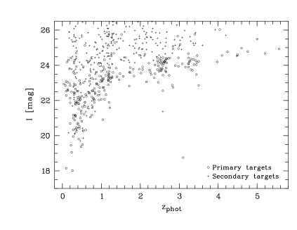
Figure 1: $I$ magnitudes as a function of the photometric redshifts of the primary (circles) and secondary extragalactic targets (crosses) of the FDF spectroscopic survey. The bright object with $z_{\rm phot}=3.1$ is the quasar Q 0130–260 ($z_{\rm spec}=3.365$).

For the present investigation we selected a sample of galaxies in the FDF covering a large range of photometric redshifts derived from the FDF photometric programme (Heidt et al. 2003b ). The photometric redshifts were calculated by fitting semi-empirical spectral energy distributions (SEDs) to the filter-band fluxes (Bender et al. BEN01 (2001), BEN04 (2004); Gabasch et al. GAB04 (2004)). The templates were constructed using stellar population models of Maraston (MARA98 (1998)) with variable reddening according to Calzetti et al. (CAL94 (1994)) and broad-band SEDs produced from photometric data of galaxies in the Hubble Deep Field North (HDF-N, Williams et al. WIL96 (1996)) with known spectroscopic redshifts. From a comparison of photometric and spectroscopic redshifts carried out in the HDF-N and the FDF we estimate for the present FDF spectroscopic sample a fraction of misidentifications of $\sim 3$ % only. The rms error of $z_{\rm phot}-z_{\rm spec}$ for the FDF objects with spectroscopically-confirmed photometric redshifts amounts to $0.13$.

To obtain sufficiently large subsamples of candidates for the different redshift intervals, apparent brightness limits for the object selection were chosen depending on the redshift. Fig. 1 shows the $I$ magnitudes (Vega system) of the spectroscopically-observed objects as a function of photometric redshift. For the redshift range $2.0$ to $4.0$ the selection limit was normally $24.5$ mag in $I$. For $I<24$ mag the fraction of the spectroscopically-observed photometric candidates was about 50 %. For lower redshifts the same level of completeness was achieved for brighter objects ($I<22.5$ mag for $1.0<z_{\rm phot}<1.5$). For $z_{\rm phot}>4.0$ one third of the objects sufficiently bright for spectroscopy ($I<25$ mag) was included.

The majority of the targets selected are intrinsically bright objects ($L>L^{*}$) at redshifts between 1 and 5. In addition to these primary targets the spectroscopic sample contains objects which were observed serendipitously as their images coincided by chance with the slit positions of the primary targets. Two or three additional objects on a slitlet were not unusual. These secondary objects constitute a random sample constrained only by the apparent brightness. Hence, faint intermediate-redshift galaxies dominate this sample, as indicated in Fig. 1.

A few high-redshift galaxy candidates were selected which deviated from the selection criteria for $z>2$ primary targets. Firstly, three Ly$\alpha$ emitters, which were initially observed as secondary targets, were converted to primary targets. Secondly, we selected three faint high-redshift candidates located in the vicinity of $z_{\rm phot}>2$ primary objects with $I<24.5$ mag. Thirdly, we included three faint objects located in the vicinity of the bright FDF quasar Q 0130–260 (see Fig. 9). These three candidates had been selected as likely Ly$\alpha$ emitters from narrow-band images sensitive to Ly$\alpha$ at the quasar redshift (see Heidt et al. 2003a ). Furthermore, three objects were selected on the basis of their photometric redshifts $z_{\rm phot}\sim 3$ and a colour excess $g-R\geq 0.5$ mag, indicating strong Ly$\alpha$ emission. In principle, these additionally selected objects increase the fraction of Ly$\alpha$ bright galaxies in the sample. However, the sample based on the standard brightness criterion is not significantly affected, since the continuum flux of the Ly$\alpha$ emission galaxies is generally low. Only two of the additional galaxies are brighter than $I=24.5$ mag. Consequently, the high-redshift sample can be considered as a representative sample for the absolute brightest objects with $z\geq 2$.

3 Observations

All spectroscopic observations of the FORS Deep Field were carried out using the two FORS instruments at the ESO VLT at Paranal, Chile, mainly between September 2000 and September 2002. The total integration time was $63.7$ h.

All spectra were taken using the multi-object spectroscopy modes MOS and MXU of FORS (see FORS Manual). The MOS masks consist of 19 individually movable and adjustable slitlets. The MXU masks are manufactured using a laser-cutting device. Since the MXU was not available for the first campaigns and only at FORS 2, almost 90 % of the exposures were obtained using the MOS mode.

To assure a homogeneous sample the observations were carried out using a standardised set-up. The slit width was uniformly set to $1^{\prime\prime}$, corresponding approximately to the size of typical high-redshift galaxies under average atmospheric conditions at Paranal. For all observations discussed here, the low-resolution grism 150 I was used. This grism covers the full range of the CCD sensitivity (3300 – 10000 Å) with a relatively high efficiency, reaching its maximum at around 5000 Å. The grism was employed without order separation filters in order to exploit the whole wavelength range and to make most efficient use of the observing time. Since most galaxies were red with no or little blue flux, second order contamination in the red was normally negligible. In the case of blue objects with significant second order contamination only the uncontaminated part of the spectrum was used. The set-up resulted in a measured spectral resolution element of $\approx 23$ Å (FWHM) for the calibration lines and $\approx 18$ Å for point sources under good seeing conditions.

Our high-redshift galaxies typically had an apparent brightness of $I>23$ mag. On the other hand, signal-to-noise ratios of 10 and more are needed for quantitative spectroscopic studies. Therefore, integration times up to 10 h were scheduled to achieve the desired S/N. The observations of the individual objects were usually distributed over several mask set-ups to optimise the observing time allocation and to reduce systematic errors caused by CCD defects and object locations near slit edges. The individual exposures had integration times between 30 and 48 min.

4 Data reduction

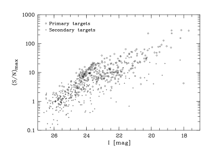
Figure 2: Continuum signal-to-noise ratio per resolution element of the FDF spectra (in the filter band $B$, $g$, $R$ or $I$ with the best average S/N) as a function of the $I$ magnitude. Circles refer to primary targets, crosses to secondary targets.

The data were reduced using MIDAS routines optimised for the reduction of FORS data, mainly based on the MIDAS context MOS.

For the bias subtraction for each observing run a master bias was generated by calculating the normalised median of a minimum of five single bias frames and subtracted from the raw frames after scaling the bias level with the overscan.

The pixel-to-pixel sensitivity variations were corrected by means of internal screen flat-fields provided by ESO for each mask set-up. Large-scale intensity fluctuations were removed by dividing the flat-fields by a smoothed version using a 50 pixel median. Then the multi-object spectra were divided by the resulting normalised flat-fields.

The wavelength calibration was carried out in two steps. First, the dispersion relation was derived using He, Hg/Cd and Ar spectra, which were obtained with the same mask configuration as the object spectra. These calibration spectra were used to obtain a fourth-order dispersion relation for each row of the MOS frame. Typical relative uncertainties of the relation were $\sim 0.5$ Å ($\sim 1/10$ pixel).

The calibration spectra were obtained in zenith position during daytime. Therefore, bending and the positioning of the laser-cut masks in the mask exchange unit (MXU) could cause variations of the slitlet locations between calibration frames and object spectra of up to one pixel. This effect was corrected by measuring the position of the prominent telluric line [O I] $\lambda\,5577$ and by shifting the spectra accordingly. The final error of the wavelength calibration was found to be about $0.5$ to 1 Å.

The sky spectrum underlying the object spectrum was derived by interpolation and subtracted. The interpolation was carried out by polynomial fits of first to third order as well as median fits using 7 to 15 pixels. In each case the most suitable approach was chosen according to its success in reaching an undistorted object continuum compatible with the photometric data and the minimisation of sky line residua. The uncertainty of the zero-flux level of the flux calibrated one-dimensional spectra was found to correspond to a few $10^{-23}\,{\rm W}\,{\rm m}^{-2}\,{\rm\AA}\,\!^{-1}$ in the optical wavelength region.

For the extraction of one-dimensional object spectra from the two-dimensional MOS spectra the S/N-optimised algorithm of Horne (HOR86 (1986)) was used. Pixels with a deviation greater than $5\,\sigma$ from the expected intensity profile were ignored in the variance-weighted summation procedure. This allows eliminating the majority of cosmics and CCD defects. As a by-product of the variance estimates the algorithm provides for each final spectrum $f(\lambda)$ an error function $\Delta f(\lambda)$ representing essentially the photon noise level.

The atmospheric extinction correction was carried out using the ESO standard extinction curve (Tüg TUG77 (1977)).

A first-order flux calibration was performed using spectra of spectrophotometric standard stars (Oke OKE90 (1990); Hamuy et al. HAM92 (1992), HAM94 (1994)) usually obtained each night with $5^{\prime\prime}$ wide slits. These spectra were reduced like the programme spectra and used to convert the ADUs into flux units. Then the flux-calibrated observed spectra were divided by the corresponding standard star spectra from the literature in order to obtain response curves. Eventually, representative correction curves were created for each run combining the individual response curves and smoothing the result by a spline interpolation.

The limited slit width of $1^{\prime\prime}$ unavoidably causes flux losses in the case of extended objects, modest seeing and/or decentred slit positions. These flux losses were corrected using the total photometric fluxes measured during the photometric programme (Heidt el al. 2003b ). In practice, quasi-photometric fluxes were calculated from the spectra (applying the known FORS filter response curves) and divided by the photometric results to determine corrections. Usually the averaged factors of the $g$ and $R$ filters were used. For very blue or very red SEDs $g$ and $R$ were substituted or supplemented by $B$ or $I$.

The resulting spectroscopic fluxes can still be affected by inaccuracies of the atmospheric extinction law, the response curve, the zero-flux level and residua of strong sky lines. For extended objects with strong colour gradients the slit loss correction can be incorrect because of systematic deviations between the measured and the representative object spectrum. To estimate the error introduced by such effects, the spectroscopic and photometric fluxes of the final co-added spectra were compared. For the primary spectroscopic targets this analysis indicates typical relative flux uncertainties of about 5 % in the $g$ and $R$ range and 15 % in the $B$ and $I$ range.

The flux-calibrated spectra were S/N-optimised co-added using the squared ratios

$$w=\frac{\langle f(\lambda)\rangle}{\langle\Delta f(\lambda)\rangle}$$ (1)

of the suitably averaged spectra $f(\lambda)$ and error functions $\Delta f(\lambda)$ as weights. At very low S/N errors of the spectral continuum level are no longer negligible, which may lead to unrealistic weights. Hence, an additional $w_{0}=0.5$ was introduced in Eq. (1), assuming that the noise levels of the individual spectra are of the same order. To remove artifacts such as CCD defects or undetected cosmics a $\sigma$-clipping procedure was carried out before the averaging routine was started. The clipping threshold was set to $6\,\Delta f(\lambda)$.

Since the detector oversampled the spectra with about 4 pixels per resolution element, all spectra were smoothed to match the spectral resolution using a Gaussian filter. The error functions were adjusted accordingly, converting noise per pixel into noise per resolution element.

Finally, the spectra were corrected for Galactic dust extinction using the law of Cardelli et al. (CAR89 (1989)) and the expected colour excess $E_{B-V}=0.018$ mag of the extragalactic objects in the FORS Deep Field (Schlegel et al. SCHL98 (1998)). In the visual the correction amounts to about 5 %.

The atmospheric B (6830 – 6950 Å) and A (7570 – 7710 Å) absorption bands were removed by dividing the spectra with a band model obtained from the average of a large number of high S/N spectra.

The resulting data set of the FDF spectroscopic survey contains 604 co-added, one-dimensional spectra, 51 % of which represent primary targets. Fig. 2 shows the S/N versus $I$ magnitude for these spectra. Primary and secondary objects are distinguished by different symbols (circles and crosses). As expected, the average S/N is higher for the primary objects ($\approx 20$) than for the secondary objects ($\approx 4$). 24 % of the spectra have a continuum S/N $\lesssim 1$. These objects, essentially all of which are secondary targets, were excluded from the further analysis.

5 Derivation of redshifts and object types

Before analysing the spectra in detail, we derived for all objects redshifts and rough object types using the following iterative procedure:

1. An approximate redshift was determined from a visual line identification.

2. An approximate object type was determined by comparison with known spectral energy distributions.

3. By averaging the spectra for each object type a set of empirical templates was constructed.

4. Improved redshifts and types were derived by cross-correlating the object spectra with these template spectra.

5. Steps (3) and (4) were repeated until an optimal fit was achieved.

In detail we proceeded as follows:

5.1 Redshifts from visually identified lines

For low-redshift galaxies with lines and blends with known rest wavelength, redshifts were determined (preferably using strong emission lines) by fitting Gaussians to the line centres. Spectra of high-redshift galaxies are characterised by resonance lines and blends with complex profiles, such as blue-shifted absorption lines and P Cygni profiles (see e.g. Adelberger et al. ADE03 (2003)). Hence, the visual redshift derivation was based on features such as the emission lines He II $\lambda\,1640$ and C III] $\lambda\lambda\,1907,1909$ and the low ionisation absorption lines Si II $\lambda\,1526$, Fe II $\lambda\,1608$. These lines were expected to represent the systemic velocities of the galaxies or outflows not larger than a few 100 km/s. Thus, our redshifts should be consistent with those of Pettini et al. (PET00 (2000)), Frye et al. (FRY02 (2002)), and Adelberger et al. (ADE03 (2003)).

5.2 Spectral definition of object types

Since most of the FDF galaxies are not resolved classification schemes based on the morphological Hubble types as applied by Kennicutt (KEN92 (1992)) and Kinney et al. (KIN96 (1996)) are not useful in our case. Therefore, we created a rough system of five galaxy spectral types (I to V) differing in the ratio of the rest-frame UV flux to the optical flux. The strengths and profiles of spectral lines have almost no impact on this classification. Obviously a one-dimensional sequence of only five types cannot be sensitive to the subtleties of the composition of the stellar population, the influence of dust and other characteristic galaxy parameters. However, in view of the greatly varying S/N of our spectra and the limited accessible wavelength range, our classification has the advantage of being rather robust to S/N induced effects.

Our classification obviously requires the presence of reliable continua. Therefore, for the strong Ly$\alpha$ emitters with weak continua a supplementary template VI was used.

QSOs (or, more generally, galaxies dominated by an active galactic nucleus), whose spectra could not be fitted by the spectral standard types I to V were allotted a special class VII.

Stars (type VIII) were identified on the basis of their angular intensity profiles and by comparison with stellar reference spectra from the literature (e.g. Pickles PIC85 (1985)). Their spectra were classified following the system of Morgan and Keenan (Morgan & Keenan MOR73 (1973); Keenan & Mc Neil KEE76 (1976)) extended to very cool objects (e.g. Martín et al. MART99 (1999)).

5.3 Calculation of the template spectra

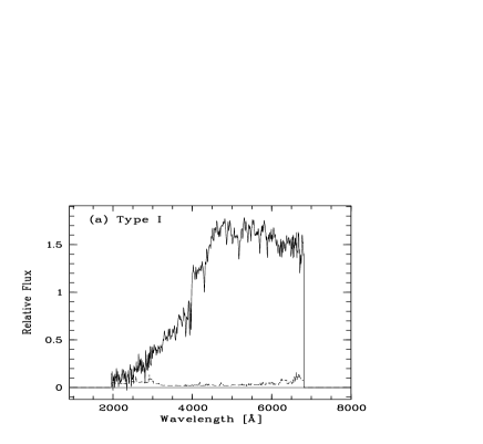
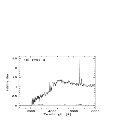
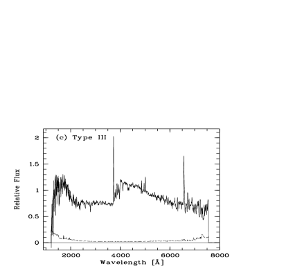
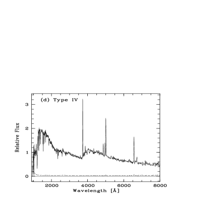
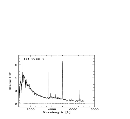
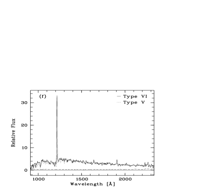
Figure 3: Empirical templates used for classifying the galaxies of the FDF spectroscopic sample. The noise level is indicated by a dashed line. SEDs I to V are normalised to the same mean flux in the wavelength range 3500 to 4500 Å. SED VI for bright Ly$\alpha$ emitters (panel (f)) is adjusted to have the mean flux of SED V between 1400 and 1600 Å. For comparison SED V is overplotted in panel (f) (dotted line).

The template spectra were calculated by averaging FDF spectra of the corresponding type with secure redshifts.

As a preparatory step the individual spectra were masked to exclude wavelength regions affected by systematic errors. The resulting useful wavelength range usually included the interval between 3800 and 8250 Å, except for regions containing strong sky line residuals. Then the spectra were converted to the rest-frame system and rebinned with a step size of 1 Å.

To obtain average spectra with equivalent widths (EWs) equal to the average EW of the individual spectra, the masked rest-frame spectra $f_{i}^{\rm m}(\lambda)$ were divided into a continuum and a line part according to

$$f_{i}^{\rm m}(\lambda)=f_{{\rm c},i}^{\rm m}(\lambda)\,f_{{\rm l},i}^{\rm m}(\lambda).$$ (2)

The $f_{{\rm c},i}^{\rm m}(\lambda)$ were generated using a median filter of 100 Å width.

The $f_{{\rm l},i}^{\rm m}(\lambda)$ were averaged as follows:

$$F_{\rm l}(\lambda)=\frac{1}{M(\lambda)}\sum_{i=1}^{n}f_{{\rm l},i}^{\rm m}(\lambda)$$ (3)

where

$$M(\lambda)=\sum_{i=1}^{n}\,m_{i}(\lambda)$$ (4)

is the sum of the mask functions $m_{i}(\lambda)$ (values either 0 or 1) of all $n$ spectra.

The continua were added sorted by redshift in order to maximise the respective size of the overlapping wavelength range. Step-by-step the summation was realised using

$$F_{{\rm c},i}(\lambda)=F_{{\rm c},i-1}(\lambda)+\frac{f_{{\rm c},i}^{\rm m}(\lambda)}{c_{i}}$$ (5)

with $F_{{\rm c},0}(\lambda)=0$, $c_{1}=1$ and the effective flux correction factor for $i\geq 2$

$$c_{i}=\bigg{\langle}\frac{M_{i-1}(\lambda)\,f_{{\rm c},i}^{\rm m}(\lambda)}{F_{{\rm c},i-1}(\lambda)}\bigg{\rangle}_{f_{{\rm c},i}^{\rm m}\,F_{{\rm c},i-1}\neq 0}$$ (6)

where

$$M_{i}(\lambda)=\sum_{j=1}^{i}m_{j}(\lambda).$$ (7)

$c_{i}$ ensures that all spectra are added with the same weight. Finally, the average continuum was calculated by

$$F_{\rm c}(\lambda)=\frac{1}{M(\lambda)}F_{{\rm c},n}(\lambda)$$ (8)

and suitably normalised.

$F_{\rm c}(\lambda)$ was derived adding spectra in ascending as well as descending redshift order. The relative deviations were smaller than 5 %. The final templates were calculated according to

$$F(\lambda)=\frac{1}{2}\big{(}F_{\rm c,\uparrow}(\lambda)+F_{\rm c,\downarrow}(\lambda)\big{)}\,F_{\rm l}(\lambda).$$ (9)

Fig. 3 shows the resulting templates for the types defined in Sect. 5.2. As shown by the figure the different types differ mainly in their ratio between the UV and optical flux. However, the nebular emission line strengths of the templates also increase from SED I (no emission) to SED V (numerous strong emission lines). Template VI, which was constructed from SED V spectra with strong Ly$\alpha$ emission, shows a similar continuum as SED V.

As they were composed from spectra of different redshift the mean spectra cover large wavelength ranges. Since different spectral regions originate from objects of different redshifts, it is clear that the mean spectra may not correspond to real galaxy spectra, if evolutionary effects are significant. Nevertheless, they are well suited for the purpose of deriving redshifts and rough object types.

5.4 Redshift derivation

To derive an accurate uniform set of redshifts, all spectra were (after conversion to a logarithmic wavelength scale) cross-correlated with their corresponding templates (see Simkin SIM74 (1974); Tonry & Davis TON79 (1979)). Only regions of the input spectra with good quality were included in the calculation. Furthermore, the continua of spectra and templates were removed to suppress the continuum background in the correlation function.

The most likely redshift was derived using a $\chi^{2}$ test checking the correspondence of the respective spectrum (continuum inclusive) and the template, with the redshift being a free parameter. This procedure takes into account that the amplitude of cross-correlation peaks depends on object type, redshift and S/N.

5.5 Final redshifts and spectral types

For each spectrum the redshift derivation procedure was carried out for each template shown in Fig. 3. Then the most probable redshift and spectral type were determined from the best fit. If the results for two templates indicated similar redshifts and fit quality, the average was taken. In general, the redshift differences were within the error limits (see below).

Since low S/N or unusual SEDs can introduce errors in automatic procedures, all results of the automatic redshift derivation were verified by visual inspection. In this way 341 redshifts could be confirmed to be obviously correct (277) or very likely (about 90 % confidence) correct (64). These objects are listed in Table 1. They represent 88 % of the primary and 23 % of the secondary targets. Considering the objects with secure redshifts only, the values are 77 % and 14 %. For the remaining 263 objects the redshift derivation was either ambiguous or no redshift could be derived because of too low a S/N.

To estimate the redshift accuracy we compared our results with those obtained from higher-resolution spectra available for part of our galaxies. For 51 brighter objects with $z<1$, we made use of medium resolution FORS-600 R spectra ($\Delta\lambda\sim 4$ Å) obtained for a different programme (see Ziegler et al. ZIE02 (2002); Böhm et al. BOH04 (2004)). The comparison indicates relative redshift errors $\Delta z/(z+1)\sim 4\times 10^{-4}$ for the 150 I spectra showing emission lines. For type I spectra, which are characterised by relatively weak absorption features, the accuracy is about $8\times 10^{-4}$.

To estimate the redshift uncertainties for all spectra, especially the high-redshift ones, the dependence of the redshift on the template used was taken into account. Moreover, redshifts were also derived by measuring spectral line positions. Taking together the different error estimates the typical relative uncertainties range between $4\times 10^{-4}$ and $10\times 10^{-4}$ depending on redshift regime, spectral type and S/N. Values for the individual redshift errors are presented in Table 1.

6 The Catalogue

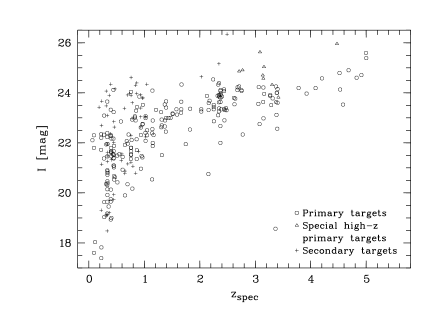
Figure 4: $I$ magnitudes as a function of the spectroscopic redshifts of the extragalactic Catalogue objects. Primary and secondary targets are indicated by circles and crosses, respectively. In contrast to Fig. 1, the special primary objects discussed in Sect. 2 are marked by triangles. The bright object with $z=3.365$ is the quasar Q 0130–260.

Table 1: Excerpt from the electronically available Catalogue of the FDF spectroscopic sample. Descriptions of the individual columns are given in the text.

No.	RA	DEC	$B$	$I$	$T_{\rm exp}$	$f/f_{0}$	S/N	$Q_{\rm s}$	Type	$z$	d$z$	$\sigma$	$Q_{\rm z}$	Rem.
	01:$\ldots$	$-$25:$\ldots$	[mag]	[mag]	[min]	[%]	(Band)					[%]
4522	06:03.8	45:42	99.0	25.4	1121	97	3.4 ($I$)	2	V	4.9996	0.0048	43	2
4573	06:04.0	46:55	25.5	23.9	281	31	3.6 ($R$)		IV	0.6993	0.0007	41	2
4609	06:04.2	46:45	25.3	23.4	135	47	4.1 ($g$)		IV	0.6431	0.0007	50	1
4654	06:04.3	47:19	22.2	20.1	30	5	4.0 ($R$)		IV	0.3989	0.0006	40	2
4657	06:04.3	43:20	21.8	19.3	120	2	8.8 ($g$)	1	III	0.2244	0.0005	36	1	600R
4662	06:04.3	43:12	25.4	24.0	240	35	3.5 ($g$)	2	V	0.7386	0.0007	50	2
4667	06:04.3	47:14	22.6	20.7	30	16	7.5 ($R$)		IV	0.4542	0.0006	32	1
4682	06:04.4	46:15	99.0	23.6	510	49	6.1 ($g$)	2	V	3.1428	0.0033	18	1
4683	06:04.4	46:51	20.2	18.6	155	54	284.2 ($g$)		VII	3.3650	0.0070		1	QSO
4684	06:04.4	48:00	25.7	23.6	30	87	2.7 ($g$)		IV	0.7843	0.0007	52	2
4685	06:04.4	43:11	25.0	23.5	240	50	9.4 ($g$)		IV	2.6254	0.0025	16	1
4686	06:04.4	45:54	22.7	21.8	442	54	43.8 ($g$)		IV	0.0943	0.0004	15	1
4691	06:04.4	48:34	25.8	24.3	550	66	13.1 ($g$)		V/VI	3.3036	0.0043	67	1	LAB
4701	06:04.5	42:52	29.4	24.7	225	60	1.4 ($I$)		V	4.9132	0.0047	82	2
4729	06:04.6	47:36	22.3	21.1	120	51	34.2 ($g$)		VIII	0			1	G
4745	06:04.6	44:03	25.2	23.8	434	67	10.2 ($g$)		V	2.6173	0.0029	17	1
4752	06:04.7	46:54	26.5	99.0	473	29	3.2 ($g$)	2	V/VI	3.3802	0.0044	119	1	LAB
4795	06:04.8	47:14	24.4	23.3	570	55	15.9 ($g$)		IV	2.1593	0.0022	14	1
4871	06:05.1	46:04	24.9	23.4	490	58	15.4 ($g$)		IV	2.4724	0.0024	13	1
4882	06:05.1	48:38	21.3	19.0	120	31	75.0 ($R$)		II	0.2777	0.0006	11	1
4910	06:05.2	46:04	25.5	24.3	120	40	2.1 ($g$)		V	0.8437	0.0007	65	2
4954	06:05.4	46:20	25.8	23.8	160	37	2.1 ($R$)		IV	0.9703	0.0008	55	2
4993	06:05.5	45:56	26.5	21.8	245	50	11.7 ($I$)		I	0.7632	0.0014	24	1
4996	06:05.5	46:28	24.4	23.3	281	56	14.6 ($g$)		IV	2.0278	0.0021	15	1

The basic properties of all 341 objects with certain or probable redshift are listed in Table 1 (in the following referred to as ‘the Catalogue’), which is available in electronic form only, except for a sample page presented in Table 1. The individual columns of the Catalogue have the following content:

No.:

Object number according to Heidt et al. (2003b ). For a few objects not listed in the photometric catalogue (mainly because no photometry could be obtained due to crowding) new numbers, starting with 9001, have been assigned.

RA:

Right ascension (equinox: 2000) in hours, minutes and seconds.

DEC:

Declination (equinox: 2000) in degrees, arcminutes and arcseconds.

B:

Total apparent $B$ magnitude (Vega system, see Heidt et al. 2003b ). Non-detections in $B$ are marked by the value $99.0$.

I:

Total apparent $I$ magnitude (as above).

$T_{\rm exp}$:

Total exposure time in minutes.

$f/f_{0}$:

Ratio between the flux which passed through the slit and the actual object flux in %. Low $f/f_{0}$ usually correspond to large object extensions. Typical values for point-like objects are around 70 %. Large values ($>80$ %) can be caused by systematic spectral errors and/or inaccurate photometry due to very low fluxes or object crowding.

S/N:

Average signal-to-noise ratio per resolution element in the filter band given in parentheses ($B$, $g$, $R$ or $I$). In each case the band with the highest S/N was selected. The S/N as a function of wavelength was calculated by dividing the object spectrum by its error function.

$Q_{\rm s}$:

Flag indicating systematic errors in the spectrum. $Q_{\rm s}=1$ refers to distorted spectra, $Q_{\rm s}=2$ to local defects.

Type:

Object type as defined in Sect. 5.2 and Fig. 3. The classes I to VI represent galaxies, VII indicates QSOs, and VIII refers to stars.

$z$:

Spectroscopic redshift.

d$z$:

Mean error of the redshift.

$\sigma$:

Relative rms deviation between spectrum and the optimal template in % of the average spectral flux.

$Q_{\rm z}$:

Quality of the redshift. $Q_{\rm z}=1$ indicates objects with secure redshifts and $Q_{\rm z}=2$ with probable redshifts ($90\,\%$ confidence level).

Rem.:

Further information on the object. For stars a rough spectral type is given. Quasars and strong Ly$\alpha$ emission galaxies are indicated by the entries ‘QSO’ and ‘LAB’ (Ly$\alpha$ bright, i.e. Ly$\alpha$ emission EW $\geq 20$ Å), respectively. ‘600R’ indicates galaxies whose redshift and object type were verified by means of the spectroscopic data of the medium resolution spectra (see Sect. 5.5).

To illustrate the sample properties Fig. 4 shows the $I$ magnitudes of the extragalactic Catalogue objects as a function of spectroscopic redshift. Primary (236) and secondary objects (63) are indicated. High-redshift primary targets, which were selected in a special way (12 objects, see Sect. 2), are marked by triangles to distinguish them from the $I$ magnitude selected primary targets, which are indicated by circles.

7 Basic properties of the spectra

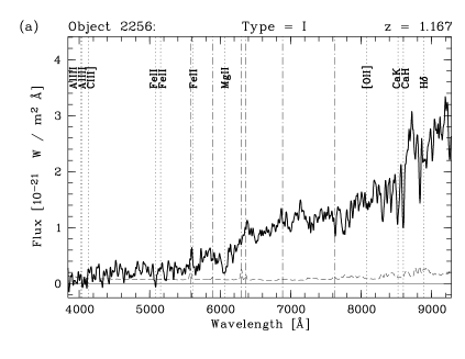
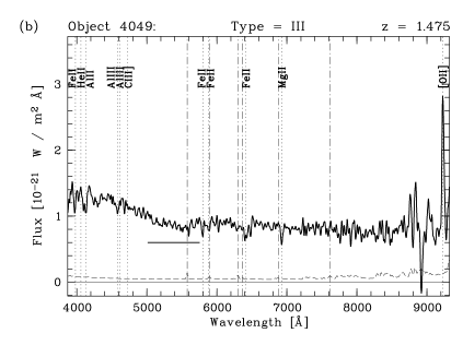
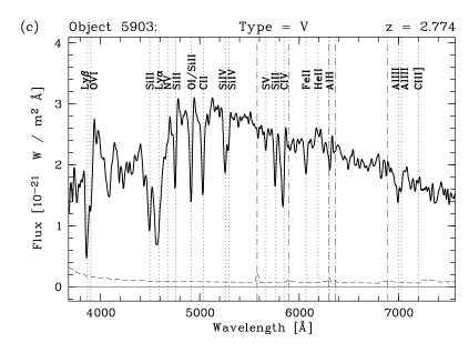
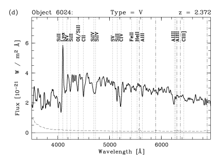
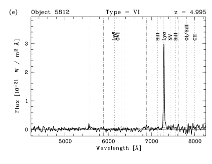
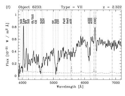
Figure 5: Examples of the FDF spectra. The positions of some prominent spectral lines are marked by vertical dotted lines. In panel (b) the position of the UV absorption feature at 2200 Å is indicated by a horizontal bar. Vertical dash-dotted lines indicate the positions where terrestrial atmospheric features ([O I] $\lambda\,5577$, Na I D, [O I] $\lambda\lambda\,6300,6364$, B band, and A band) were removed. The noise level is indicated by a dashed line. At the top of each diagram the object number, the spectral type, and the redshift are given.

In addition to the catalogue the flux-calibrated individual object spectra with reliable redshifts and no strong systematic errors are also available as an electronic atlas. In the following we describe some properties of these spectra.

7.1 Stars

The FDF spectroscopic sample contains 42 stars of spectral types G to L. Most frequent are K stars (18). Five stars have spectral types later than M5. None of the stars is brighter than 17 mag in $I$. Since the FDF is located close to the South Galactic Pole, most of the observed stars must belong to the halo or the thick disk.

7.2 Galaxies

The spectra of the 158 galaxies with $z<1$ show a great variety of spectral types ranging from ellipticals to extreme starburst galaxies.

Since early-type galaxies are intrinsically red, it is difficult to find such objects with high redshifts in optical surveys. For $z>1.3$ the 4000 Å break is shifted beyond our spectral window. This readily explains why no type I galaxy beyond $z=1.17$ (FDF-2256, see Fig. 5(a)) could reliably be identified in the FDF, so far, and why only six candidates of spectral type I or II with $z\geq 1$ were detected.

Some of the intermediate redshift galaxies show a depression at about 2200 Å (rest frame). As an example FDF-4049 is presented in Fig. 5(b). The 2200 Å feature of this galaxy corresponds to $E_{\rm B-V}\approx 0.15$ mag if a Galactic extinction law is assumed. The figure seems to illustrate that the well-known broad dust absorption feature, which is thought to be caused by small carbon-rich particles (see Cardelli et al. CAR89 (1989)), is also present in at least part of the intermediate-redshift galaxies.

In the rest-frame wavelength range between 2000 and 3700 Å galaxy spectra are poor in prominent spectral lines. This complicates the derivation of reliable redshifts in the range between $1.5$ and 2. Therefore, in this redshift range secure redshifts could be derived for two objects only.

For $z\geq 2$ we observe only starburst galaxies. Their spectra are dominated by the Ly$\alpha$ line (with profiles ranging from strong absorption to strong emission), the absorptions of the Ly$\alpha$ forest short-ward of 1216 Å, and the spectral break of the Lyman limit at 912 Å. Furthermore, the spectral region red-ward from Ly$\alpha$ is marked by numerous lines, usually showing absorption profiles, and often of interstellar origin (e.g. lines of Si II and C II). Except for Ly$\alpha$ significant emission could be detected in a few cases only, either in the form of a P Cygni profile (e.g. C IV $\lambda\lambda\,1548,1550$) or as pure emission (e.g. He II $\lambda\,1640$ and C III] $\lambda\lambda\,1907,1909$). All these features are visible in the spectra of FDF-5903 (Fig. 5(c)) and FDF-6024 (Fig. 5(d)).

Four (44 %) of the nine galaxies with $z\gtrsim 4.5$ were found to be Ly$\alpha$ bright (type VI). This percentage is comparable to the redshift range $3<z<4$ where about 37 % are LABs. Up to now, the objects with the highest spectroscopic redshifts in the FDF are the galaxies FDF-4522 and FDF-5812 (Fig. 5(e)) both having $z\approx 5.0$.

7.3 Quasars

Most of the eight quasars at redshifts between $0.865$ and $3.365$ identified in the FDF show normal QSO spectra dominated by broad emission lines of Ly$\alpha$, N V, Si IV, C IV, C III] and/or Mg II. The only exception is FDF-6233 at $z=2.32$ (see Fig. 5(f)) which belongs to the rare class of broad absorption line quasars (BAL, e.g. Menou et al. MEN01 (2001)). Its spectrum is dominated by strong, broad, blue-shifted absorption troughs of Si IV, C IV and Al III indicating outflows of several 1000 km/s. Ly$\alpha$, N V, and C III] show relatively narrow emission components. In contrast to the other quasars the continuum of FDF-6233 decreases rapidly short-ward of 1750 Å (rest frame).

8 Distribution of spectroscopic redshifts

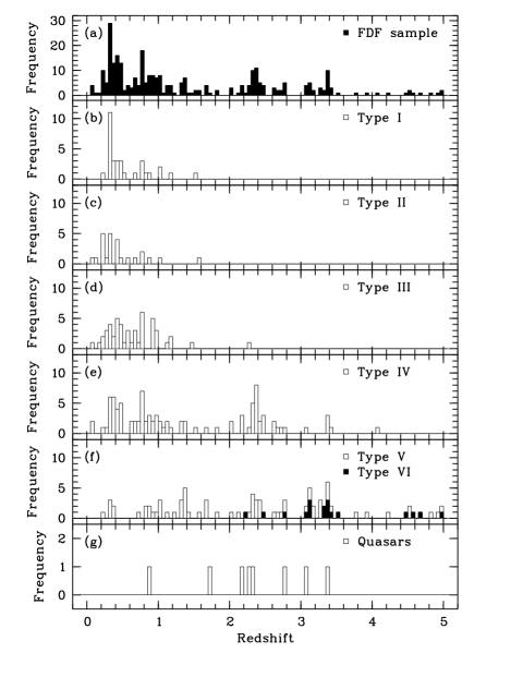
Figure 6: Redshift distribution of the FDF spectroscopic sample for (a) the complete Catalogue (see Sect. 6), (b) – (f) galaxies of different object type (see Fig. 3) and (g) the quasars. In diagram (f) galaxies of type V (white bars) as well as type VI (black bars) are plotted. The redshift resolution is $\Delta z=0.05$.

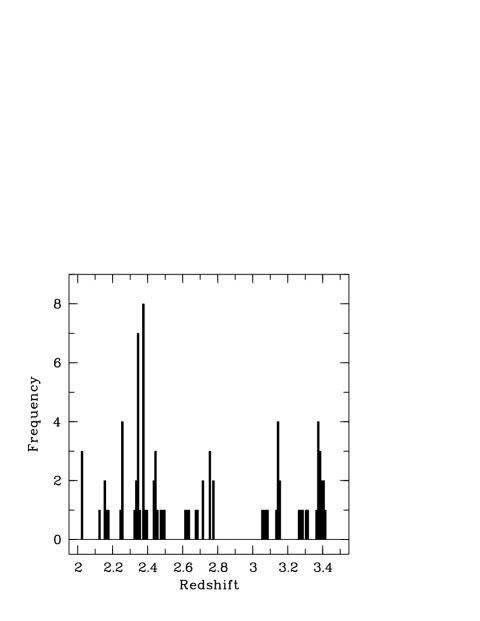
Figure 7: Redshift distribution of the FDF spectroscopic sample in the range $2<z<3.5$ plotted with a redshift resolution of $\Delta z=0.01$.

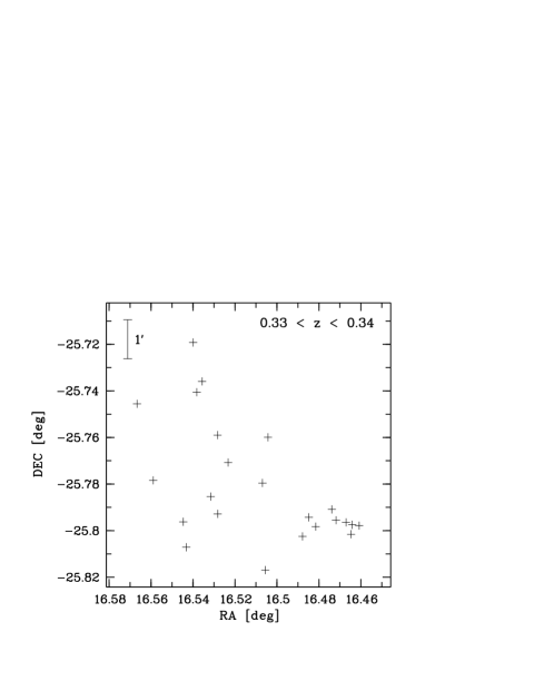
Figure 8: Distribution of galaxies within the range $0.33<z<0.34$ in the FDF.

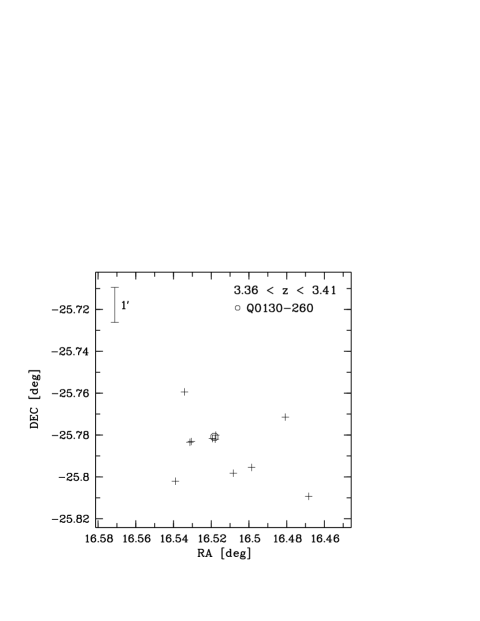
Figure 9: Distribution of galaxies within the range $3.36<z<3.41$ in the FDF. The position of the quasar Q 0130–260 is indicated by a circle. The three objects close to the quasar are strong Ly$\alpha$ emitters, which were selected using narrow-band images (see Sect. 2).

Fig. 6(a) shows the spectroscopic-redshift distribution of the galaxies and QSOs with a resolution of $\Delta z=0.05$. Significant local maxima are evident at $z=0.325$ (29 objects), $z=0.775$ (18), $z=2.375$ (11) and $z=3.375$ (10). In part this clustering of redshifts had already been noticed in the distribution of the photometric redshifts. In some cases the overdensities extend over more than two bins. For instance, the three adjacent bins comprising the redshift range between $2.30$ and $2.45$ contain 26 objects which represent about 27 % of the $z\geq 2$ sample. On the other hand, the peak around $z=0.325$ is mainly produced by a redshift interval ranging from $0.331$ to $0.339$ ($\langle z\rangle=0.335$, $\sigma_{z}=0.002$) which is smaller than the bin size but which includes 23 galaxies. As indicated in Fig. 7 such fine structure of the redshift distribution is also present at high redshifts. An example is the narrow redshift range between $2.372$ and $2.378$ ($\langle z\rangle=2.374$, $\sigma_{z}=0.002$) which includes eight galaxies, or about 73 % of the objects within the standard bin around $z=2.375$ (see above). As pointed out by Frank et al. (FRA03 (2003)) the high-redshift galaxy overdensities correlate well with QSO metal absorption line systems in the direction of the FDF. Besides the striking peaks, there are also indications of marked gaps in the redshift distribution. At low redshifts this is particularly evident around $z=0.525$ where the redshift distribution reaches a local minimum. At high redshifts a lack of galaxies exists between $2.80$ and $3.05$, where no objects could be detected, so far. The relatively low number of objects between $1.5$ and $2.0$ is a consequence of the difficulty to identify galaxies in this redshift range from visual spectra (see Sect. 7.2).

Since the spectroscopic sample is representative for the most luminous objects at each redshift (see Sect. 2), the observed distribution can (apart from the redshift range $1.5<z<2.0$) be assumed to be representative of the real distribution for the absolutely bright objects in the direction of the FDF. On the other hand, we have almost no information on the distribution of the intrinsically faint $z>2$ objects ($M_{\rm B}>-20$ mag), as such objects are rare in our sample.

Since the first photometric observations of the FDF a (poor) cluster is known to be located in the southwestern corner of the field (see Heidt et al. 2003b , Ziegler et al. ZIE04 (2004)). This cluster contributes to the peak of the FDF redshift distribution at $z\approx 0.335$. As indicated by Fig. 8 the other objects at this redshift are not randomly distributed either, as no single object of this redshift is found in the northwestern corner of the FDF. For the other peaks no significant deviation from a random distribution over the area of the FDF could be detected. This negative result may in part be due to the insufficient number of objects. But, since the angular size of the FDF covers just about the size of a large galaxy cluster at high redshift no major angular clustering effects were expected. Nevertheless, some indications for clustering on small scales were found. For instance, the galaxies between $z=3.36$ and $3.41$ populate the southern part of the FDF only (Fig. 9). Furthermore, three Ly$\alpha$ emitters of this redshift were found less than $5^{\prime\prime}$ from the bright quasar Q 0130–260. Moreover, several close pairs of galaxies with similar redshifts were discovered. In one case a dense group at $z\approx 2.347$, comprising four members (FDF-5135, 5165, 5167, 5190), was identified. The mutual distances of these objects are $<3^{\prime\prime}$.

In general, the FDF spectroscopic data, indicating predominantly moderate clustering of galaxies up to high redshifts, which can be attributed to large-scale structure, agree well with earlier results of, e.g., Adelberger et al. (ADE98 (1998)), Steidel et al. (STE98 (1998)), or Cohen et al. (COH00 (2000)).

Table 2: Distribution of objects with reliable redshifts in the FDF spectroscopic sample. The table indicates for each type the total number of objects $N$, the median redshift $\overline{z}$, the average redshift $\langle{}z\rangle$ and its variance $\sigma_{z}$.

Type	$N$	$\overline{z}$	$\langle{}z\rangle$	$\sigma_{z}$
I	32	0.4	0.6	0.3
II	25	0.3	0.5	0.3
III	50	0.6	0.7	0.4
IV	96	1.0	1.4	1.0
V + VI	88	2.4	2.4	1.3
QSOs	8	2.3	2.3	0.8
Extragalactic	299	0.9	1.4	1.2
objects
Stars	42	–	–	–

The redshift distribution of the different object types defined in Sect. 5.2 and 5.3 is shown in Fig. 6(b)–(g). The type-dependent median and mean redshifts are presented in Table 2. For the reasons outlined above the types I and II are concentrated at low redshifts (median values $0.4$ and $0.3$). Furthermore, type I shows a strong overdensity at $z\approx 0.335$ where 11 of 32 early-type galaxies are located. This obviously reflects the predominance of E and S0 galaxies in the cluster at this redshift. The change of the apparent composition of object types with redshift due to the redshift-dependent selection bias is particularly obvious for class V/VI: At low redshifts this type plays a minor role (7 % of the observed objects at $z<0.5$), but at high redshifts type V/VI becomes the dominating class. At $2\leq z<3$ the extreme starburst galaxies contribute 38 % to all identified objects, at $3\leq z<4$ they present 78 % and at $z\geq 4$ the fraction increases to 91 % (10 of 11 objects).

9 Exploring evolutionary effects

A detailed discussion of the whole FDF spectroscopic sample is beyond the scope of this paper. Instead, we will focus on some properties of the high-redshift objects. As average spectra of spectroscopic subsamples selected by redshift and/or spectral type are known to be well suited to investigate the characteristic properties of galaxy populations, the following discussion is based mainly upon such mean spectra. An analysis of individual object spectra can be found in, e.g., Mehlert et al. (MEH02 (2002)) and Tapken et al. (TAP04 (2004)).

9.1 The calculation of composite spectra

Composite spectra of FDF subsamples were calculated using similar procedures as used by S (03) to facilitate a comparison with their spectroscopic sample (see Sect. 9.4). In detail, the flux-calibrated, co-added spectra (see Sect. 4) were shifted to the vacuum rest frame, rebinned to a scale of 1 Å per pixel, scaled to a common mode in the wavelength range between 1250 and 1500 Å, and finally averaged unweighted to get a representative average.

The averaging of spectra showing different continuum levels may lead to a systematic change of the mean equivalent width of spectral lines. A comparison with mean spectra based on the alternative method described in Sect. 5.3 showed that for Ly$\alpha$ an overestimate of the true EW of the order 10 % can occur. For other lines no significant effect could be detected. The dependence of the Ly$\alpha$ strength on the normalisation method must be kept in mind when analysing the results described in the following (see Sect. 9.5).

In contrast to S (03), we did not exclude extreme flux values during the averaging. Instead, our averaging procedure omitted wavelength ranges affected by significant sky line residuals.

9.2 The overall mean spectrum of the high-redshift sample

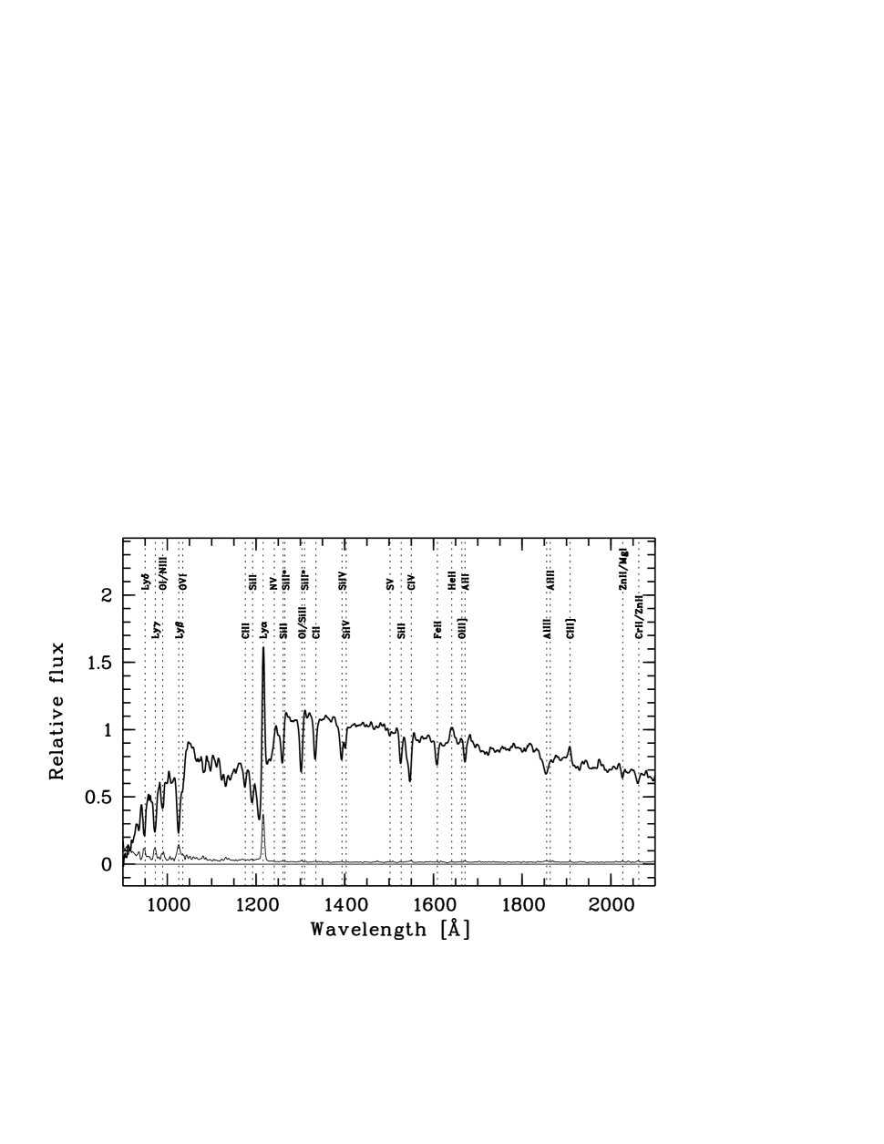
Figure 10: Composite spectrum of 64 FDF galaxy spectra with S/N $\geq 4$ in the range $2<z<4$ (thick solid line). The positions of prominent UV lines are indicated. The thin solid line at the bottom of the spectrum gives the mean error of the average spectrum as derived from the scatter of the individual spectra. Outside strong spectral features this error agrees with the value expected from the observational errors. In the case of some strong features such as Ly$\alpha$ the mean error is dominated by the physical variance in the individual spectra.

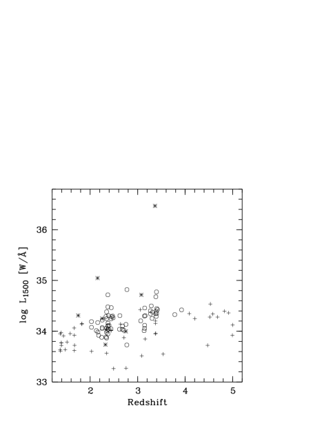
Figure 11: Luminosities at 1500 Å of the $z>1.35$ FDF galaxies as a function of redshift. To derive the luminosity the spectral flux was measured in the wavelength interval 1480 to 1520 Å. Galaxies used for the calculation of the composite spectra are indicated by circles. The remaining high-redshift objects are marked by crosses apart from QSOs, which are indicated by asterisks.

In Fig. 10 we present a composite of 64 galaxy spectra with $2<z<4$ and a continuum S/N $\geq 4$. This subsample of photometrically selected objects ($I\lesssim 24.5$ mag) represents about 91 % of all galaxies with secure redshift in the range $2<z<4$. All objects are primary targets (see Sect. 2). Three $z>3$ galaxies (FDF-7452, 7644, 8215) were initially included in the observations because of suspected Ly$\alpha$ emission. One $z>3$ object (FDF-4691) was originally a secondary target showing strong Ly$\alpha$ emission. One $z<3$ object (FDF-9011) was included due to its location close to another sample galaxy. The individual spectra are representative of the integrated light of the entire galaxies, since the slit losses are not more than twice those for point-like objects (see Sect. 6). The mean redshift of this subsample is $\langle z\rangle=2.72$ ($\sigma_{z}=0.49$). The UV luminosities at 1500 Å of the selected galaxies (derived from the flux in the interval 1480 to 1520 Å) are indicated by circles in Fig. 11. $\langle\log L_{1500}[{\rm W/\AA}]\rangle$ amounts to $34.22$ ($\sigma_{L}=0.22$).

The composite spectrum reaches a continuum S/N $\approx 60$, which allows a comparison with similar high-S/N high-redshift spectra from the literature (e.g. Pettini et al. PET00 (2000); S (03)). While the general character of all these spectra is similar, differences in spectral details, such as the Ly$\alpha$ strength and the continuum slope, are evident. We discuss these differences in Sect. 9.4.

9.3 The redshift dependence of spectral properties

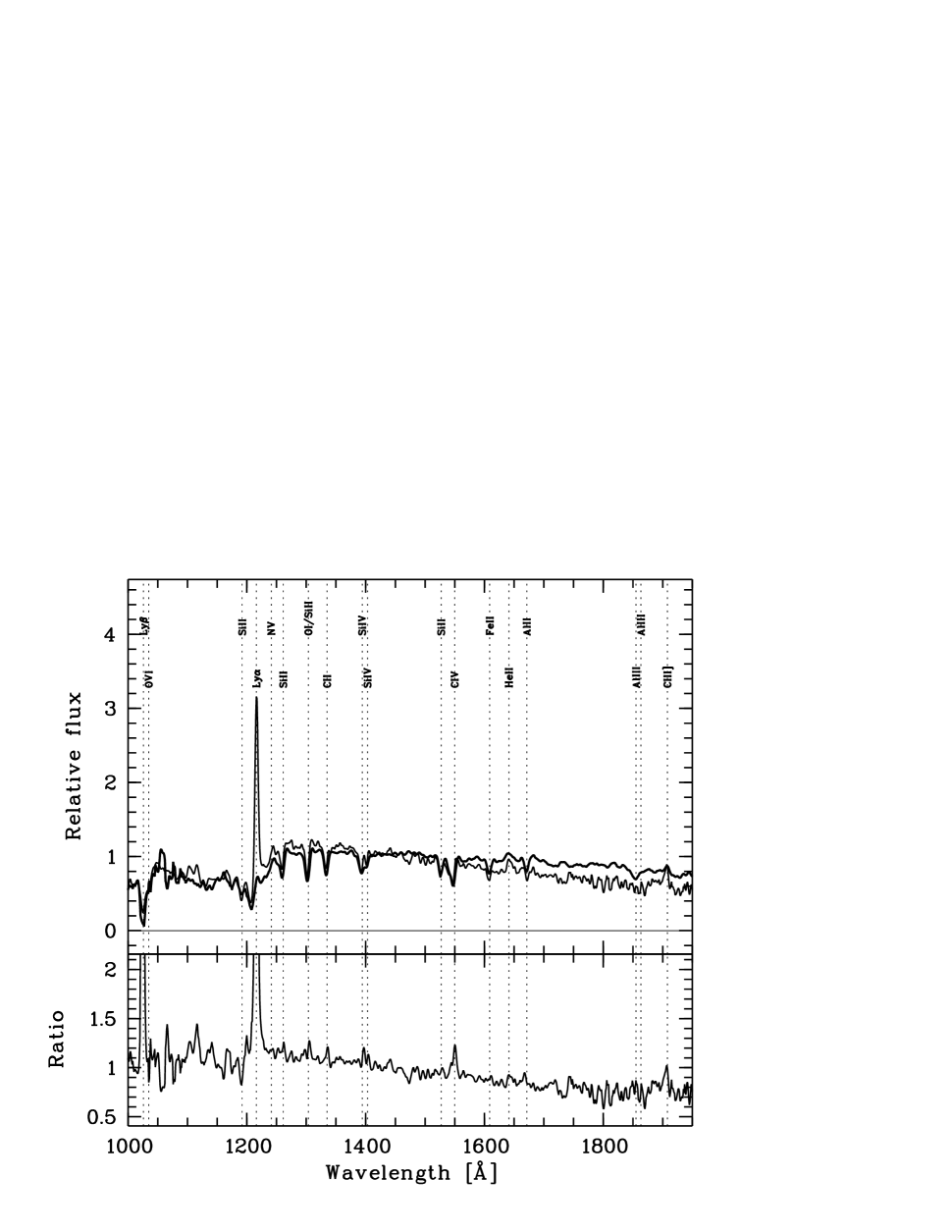
Figure 12: Comparison of FDF composite spectra covering the redshift intervals $2<z<3$ (thick line) and $3<z<4$ (thin line), respectively. The lower panel gives the ratio of the $3<z<4$ and the $2<z<3$ composite spectrum. The positions of prominent lines are indicated.

Table 3: Properties of the FDF composite spectra representative of the redshift ranges $2<z<3$ and $3<z<4$ in comparison. The table lists the number of spectra averaged, the mean redshift, the average luminosity at 1500 Å (see Sect. 9.2), the Ly$\alpha$ equivalent width, the continuum slope $\beta$, the mean equivalent width of low ionisation interstellar absorption lines (see Fig. 16) and the EWs of C IV $\lambda\lambda\,1548,1550$, He II $\lambda\,1640$ and C III] $\lambda\lambda\,1907,\,1909$. All errors given are mean errors (see Sect. 9.1).

$z$ range	$2-3$	$3-4$
$N$	$42$	$22$
$z$	$2.39\pm 0.03$	$3.33\pm 0.04$
$\log L_{1500}[{\rm W/\AA}]$	$34.14\pm 0.03$	$34.35\pm 0.04$
$W_{\rm Ly\alpha}$ [Å]	$6.90\pm 2.10$	$-10.20\pm 6.10$
$\beta$	$-0.56\pm 0.11$	$-1.79\pm 0.13$
$W_{\rm LIS}$ [Å]	$1.98\pm 0.10$	$1.55\pm 0.15$
$W_{\rm C\,IV}$ [Å]	$3.80\pm 0.25$	$2.33\pm 0.35$
$W_{\rm C\,III]}$ [Å]	$-1.10\pm 0.30$	$-3.40\pm 0.70$
$W_{\rm He\,II}$ [Å]	$-1.30\pm 0.20$	$-2.20\pm 0.40$

To investigate evolutionary effects in our sample we computed in the next step mean spectra of the galaxies within the redshift intervals $2<z<3$ and $3<z<4$. The resulting composite spectra with mean redshifts $\langle z\rangle=2.39$ ($\sigma_{z}=0.19$) and $\langle z\rangle=3.33$ ($\sigma_{z}=0.20$) are based on 42 and 22 objects, respectively. The results are given in Fig. 12 and Table 3.

Following the normal spectroscopic convention in Table 3 (and throughout this paper) for net absorption lines we give positive equivalent width values, while net emission features are characterised by negative EW features. The EW mean errors were estimated on the basis of the mean errors of the composite spectra, which were derived from the scatter of the continuum-subtracted individual spectra, and the uncertainties concerning the continuum level determination. In contrast, the mean errors of the continuum slope $\beta$ (calculated in the range 1200 to 1800 Å assuming $f(\lambda)\propto\lambda^{\beta}$ following Leitherer et al. (LEI02 (2002))) were derived from the scatter of the values measured in the individual galaxy spectra (see Fig. 21). Usually the $\beta$ of the mean spectrum and the average $\beta$ of the individual spectra were roughly the same, differing by less than $0.1$, which shows that the composite spectra are characteristic for the respective samples, at least with regard to the continuum slope.

As shown by Fig. 12 and Table 3, the $2<z<3$ mean spectrum has a rather flat continuum ($\beta=-0.56\pm 0.11$) and Ly$\alpha$ emission is weak ($W_{\rm Ly\alpha}=+7\pm 2$ Å). In contrast, the $3<z<4$ mean spectrum shows a steep UV continuum ($\beta=-1.79\pm 0.13$) and strong Ly$\alpha$ emission ($W_{\rm Ly\alpha}=-10\pm 6$ Å). The equivalent widths of the majority of spectral lines and in particular all interstellar absorption lines show minor differences only. However, in general, the EWs tend to be higher in the lower redshift range. A strong redshift dependence is observed for the C IV resonance doublet, which shows a weaker absorption at higher redshifts (as noted already by Mehlert et al. MEH02 (2002)). Furthermore, C III] displays a stronger emission in the $3<z<4$ mean spectrum. However, due to the line’s location in the region of strong OH bands at $z>3$ the $3<z<4$ spectrum contains only five spectra at C III]. Therefore, the observed increase of C III] with redshift may not be statistically meaningful.

The composite spectrum of the higher redshift range ($3<z<4$) includes only few objects with luminosities lower than $\log L_{1500}=34.2$ (3 out of 22; see Fig. 11), whereas 28 out of 42 objects in the range $2<z<3$ are below this value. To check the effect of the luminosity difference on the spectral properties, we also calculated composite spectra with $\log L_{1500}=34.2$ as lower luminosity limit. The results showed that the luminosity does not affect the spectral differences, except perhaps for a slight decrease of the Ly$\alpha$ strength in the high-luminosity subsample (from $-10\pm 7$ Å to $-5\pm 6$ Å), caused by the omission of two strong Ly$\alpha$ emitters.

9.4 Comparison with the composite spectrum of Shapley et al.

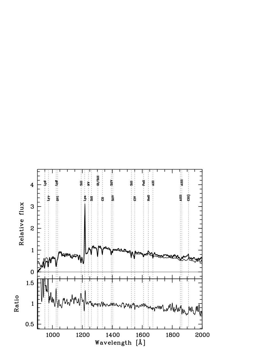
Figure 13: Comparison of composite spectra representative of the FORS Deep Field in the redshift range $2.5<z<3.5$ (thick line) and the S03 sample at $z\sim 3$ described in Steidel et al. (STE03 (2003)) and S (03) (thin line). The original S03 mean spectrum was smoothed to the same spectral resolution and normalised to the same mean continuum level in the interval $1250-1500$ Å. The lower panel gives the ratio between the FDF and the S03 composite spectra.

S03 have published a composite spectrum of a homogeneous sample of almost 1000 Lyman-break galaxies at $z\sim 3$ selected via the Lyman-break technique (see Steidel et al. STE03 (2003)). Because of the different selection criteria, the redshift distributions of the FDF galaxies ($\langle z\rangle=2.72$, $\sigma_{z}=0.49$) and the S03 sample ($\langle z\rangle=2.96$, $\sigma_{z}=0.29$) differ. 53 % of the FDF high-redshift galaxies are at $z<2.5$, whereas this redshift range is essentially absent in the S03 sample. Hence, in view of the results of Sect. 9.3, differences in the spectral properties are to be expected. Therefore we calculated a composite spectrum of 28 FDF galaxies between $z=2.5$ and $3.5$ with a similar redshift coverage ($\langle z\rangle=3.11$, $\sigma_{z}=0.28$) as the S03 sample. Fig. 13 compares this composite spectrum with the S03 spectrum. The Ly$\alpha$ strength ($W_{\rm Ly\alpha}=-9\pm 5$ Å) as well as the continuum slope ($\beta=-1.54\pm 0.13$) of the $2.5<z<3.5$ spectrum show good agreement with the S03 values ($W_{\rm Ly\alpha}=-11$ Å and $\beta=-1.81$). This shows that samples with comparable redshift distributions have similar average spectra independent of the selection method.

The fact that the average apparent brightness of the S03 sample ($R_{\rm Vega}\approx 24.38$ mag, converted from $R_{\rm AB}$) is somewhat lower than that of the $2.5<z<3.5$ FDF sample ($R_{\rm Vega}=24.19\pm 0.11$ mag) apparently has no effect on the average spectra. This is confirmed by a comparison of the composite spectra of the bright ($\langle R\rangle=23.80$ mag) and the faint half ($\langle R\rangle=24.58$ mag) of the $2.5<z<3.5$ sample, which show very similar spectra. The only possible difference may be a moderately higher Ly$\alpha$ emission of $-16\pm 10$ Å for the faint subsample in comparison to $-3\pm 4$ Å for the bright subsample.

9.5 Relations between Ly$\alpha$ emission and other spectral properties

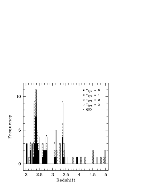
Figure 14: Redshift distribution of FDF galaxies with different Ly$\alpha$ types (see legend). The presence of a quasar at the corresponding redshift is marked by an asterisk.

Table 4: Distribution of Ly$\alpha$ types $T_{\rm Ly\alpha}$ (as defined in Sect. 9.5) among the FDF high-redshift galaxies ($2<z<5$). For each Ly$\alpha$ class the total number of objects $N$, the median redshift $\overline{z}$, and the mean redshift $\langle z\rangle$ with its standard deviation $\sigma_{z}$ are given.

$T_{\rm Ly\alpha}$	$N$	$\overline{z}$	$\langle{}z\rangle$	$\sigma_{z}$
0	36	2.4	2.6	0.5
1	14	2.3	2.9	0.9
2	24	3.1	3.1	0.8
3	18	3.3	3.5	0.8

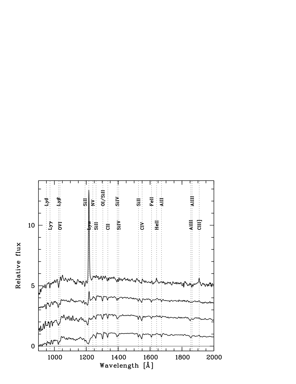
Figure 15: Comparison of FDF composite spectra representative of different Ly$\alpha$ types ranging from strong emission ($T_{\rm Ly\alpha}=3$, uppermost spectrum) to pure absorption ($T_{\rm Ly\alpha}=0$, lowest spectrum). The spectra are normalised and shifted by multiples of $1.0$ relative flux units.

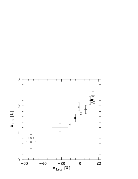
Figure 16: The dependence of the strength of low-ionisation lines on the Ly$\alpha$ equivalent width. $W_{\rm LIS}$ is the average EW of the six strong low-ionisation features Si II $\lambda\,1260$, OI/SiII $\lambda\,1303$, C II $\lambda\,1334$, Si II $\lambda\,1526$, Fe II $\lambda\,1608$, and Al II $\lambda\,1670$. The individual symbols represent the values measured in the FDF composite spectra for different Ly$\alpha$ strengths and redshift ranges. Open circles show the values for the redshift range $2<z<4$. Filled squares and triangles represent the smaller ranges $2<z<3$ and $3<z<4$, respectively. The $1\,\sigma$ error bars include the variance between the individual spectra and the errors of the continuum level definition. For comparison the corresponding data from S (03) are also included (crosses).

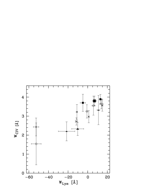
Figure 17: The dependence of the strength of C IV on the Ly$\alpha$ equivalent width. The smaller symbols are as in Fig. 16. The big filled square, filled triangle, and cross show the EWs measured in the $2<z<3$, $3<z<4$, and the S03 composite spectrum, respectively.

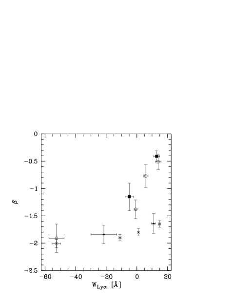
Figure 18: The dependence of the strength of the continuum slope parameter $\beta$ (see Leitherer et al. LEI02 (2002)) on the Ly$\alpha$ equivalent width. Symbols are as in Fig. 16. The $\beta$ uncertainties were obtained from the scatter of the values derived for the individual spectra. The values given in S (03) were calculated from the colour excess $E_{\rm B-V}$, whereas the FDF values were derived by fitting the composite spectra. Hence, the S03 values (crosses) were corrected assuming a constant offset. The shift ($\Delta\beta=-0.92\pm 0.05$) was estimated from the $\beta$ measured in the published composite spectrum of the total S03 sample.

Figure 19: The dependence of the strength of C III] $\lambda\lambda\,1907,\,1909$ on the Ly$\alpha$ equivalent width. The open circles represent the values measured in the FDF composite spectra for different Ly$\alpha$ strengths. For comparison the corresponding data from S (03) are also included (crosses).

Figure 20: The dependence of the strength of He II $\lambda\,1640$ on the Ly$\alpha$ equivalent width. The open circles represent the values measured in the FDF composite spectra for different Ly$\alpha$ strengths. The cross indicates the He II equivalent width of the composite spectrum of the S03 sample.

In part of our spectra the Ly$\alpha$ line occurs in emission. The emission originates from recombination of hydrogen ionised either by hot stars or by an AGN. The escape of Ly$\alpha$ photons is hampered by multiple resonance scattering resulting in large path lengths through the galaxy (see Charlot & Fall CHA93 (1993)). Hence, the Ly$\alpha$ emission is very sensitive to the dust content and the geometry and structure of the H I velocity field (see e.g. Kunth et al. KUN98 (1998)).

To study the relation between the Ly$\alpha$ emission and other spectral features we divided the high-redshift galaxy sample spectra into four classes according to the EW of the Ly$\alpha$ emission component $W_{{\rm Ly\alpha},{\rm e}}$. The four classes ($T_{\rm Ly\alpha}$) were defined in the following way:
$T_{\rm Ly\alpha}=0$: No (detectable) emission.
$T_{\rm Ly\alpha}=1$: Very weak emission (not measurable).
$T_{\rm Ly\alpha}=2$: $2\,{\rm\AA}\leq-W_{{\rm Ly\alpha},{\rm e}}<20$ Å.
$T_{\rm Ly\alpha}=3$: $-W_{{\rm Ly\alpha},{\rm e}}\geq 20$ Å.

Mean and median redshifts of the individual Ly$\alpha$ classes are listed in Table 4. The resulting redshift distribution of the different types is shown in Fig. 14. The histogram indicates a conspicuous evolution of the typical Ly$\alpha$ characteristics from $z=2$ to 5. At redshifts $2<z<3$ only 26 % of the objects shows significant Ly$\alpha$ emission ($T_{\rm Ly\alpha}\geq 2$). Only 3 of 18 Ly$\alpha$-bright galaxies (LABs, $T_{\rm Ly\alpha}=3$) are at $z<3$. They represent 6 % of all galaxies in the range $2<z<3$. At higher redshifts the fraction of galaxies with $T_{\rm Ly\alpha}\geq 2$ increases to 67 % at redshifts $3<z<4$ and 73 % at $4<z<5$. Considering the galaxies with strong Ly$\alpha$ emission only, the corresponding values are 37 % and 36 %. Hence, the evolution of the average Ly$\alpha$ strength between $z=3.3$ and $2.4$ is caused by a change of the frequency and the strength of Ly$\alpha$ emission, if present.

For the analysis of the correlation of Ly$\alpha$ strength with other spectral features, we again took the 64 galaxy spectra in the range $2<z<4$ and calculated composite spectra for each of the four Ly$\alpha$ classes introduced above. In Fig. 15 the resulting spectra are plotted. To investigate the redshift dependence of the correlations, four further composite spectra were calculated, differing in redshift range ($2<z<3$ and $3<z<4$) and Ly$\alpha$ class $T_{\rm Ly\alpha}$ ($0-1$ and $2-3$). To avoid too small numbers of spectra in individual composite spectra, the Ly$\alpha$ types were grouped into two categories only. For all composite spectra EWs and continuum slopes were measured, allowing us to check whether the FDF sample follows the relations found by S (03).

As pointed out by Pettini et al. (PET00 (2000)) and S (03), prominent low-ionisation absorption lines of interstellar origin in spectra of high-redshift galaxies (like OI/SiII $\lambda\,1303$ and Si II $\lambda\,1526$) are normally saturated. The EWs of such lines are mainly determined by the product of the covering fraction of the neutral gas clouds and the velocity field, which makes them suitable indicators of the geometry and kinematics of neutral gas in high-redshift galaxies. Fig. 16 shows the average EW of six prominent low-ionisation features as a function of the Ly$\alpha$ equivalent width $W_{\rm Ly\alpha}$. The four data points of the different Ly$\alpha$ types (open circles) indicate a significant decrease of $W_{\rm LIS}$ with increasing $W_{\rm Ly\alpha}$. The spectrum representing the strong Ly$\alpha$ emitters shows a $W_{\rm LIS}$ more than three times weaker than does the spectrum with pure Ly$\alpha$ absorption, in close agreement with the results of Shapley et al. (crosses). Moreover, significant differences of the relations for $2<z<3$ (filled squares) and $3<z<4$ (filled triangles) cannot be detected, which suggests that a redshift dependence, if present, must be weak. Consequently, Fig. 16 suggests a strong dependence of the Ly$\alpha$ strength on the geometry and kinematics of the H I clouds (in accordance with Kunth et al. KUN98 (1998)) independent of the redshift.

Fig. 17 shows C IV $\lambda\lambda\,1548,\,1550$ as a function of the Ly$\alpha$ strength. As C IV originates primarily in photospheres and winds of luminous hot stars (Walborn et al. WAL95 (1995); Heckman et al. HEC98 (1998)) and the wind power depends on the metallicity, $W_{\rm C\,IV}$ is a good metallicity indicator (Leitherer et al. LEI01 (2001)). The figure confirms the strong dependence of the C IV strength on the redshift, noted already by Mehlert et al. (MEH02 (2002)). On the other hand, only a weak dependence of $W_{\rm C\,IV}$ on $W_{\rm Ly\alpha}$ is indicated. The large $W_{\rm C\,IV}$ mean errors suggest a marked scatter of the C IV strength for each Ly$\alpha$ type. Consequently, the Ly$\alpha$ emission appears to be rather independent of metallicity-dependent stellar wind properties.

In Fig. 18 we investigate the dependence of the continuum slope $\beta$ on $W_{\rm Ly\alpha}$. As discussed in Sect. 9.6, $\beta$ essentially traces the attenuation of hot star continua by interstellar dust. The diagram reveals a conspicuous redshift dependence of the $\beta-W_{\rm Ly\alpha}$ relation. The galaxies at $z<3$ (filled squares), which represent the main contribution to the FDF $2<z<4$ sample (open circles), show a strong dependence of the continuum slope and Ly$\alpha$. In contrast, the galaxies at $z>3$ (filled triangles) indicate a rather weak $\beta-W_{\rm Ly\alpha}$ correlation, resembling the relation for the S03 sample (crosses). The S03 $\beta$ values had to be corrected (see Fig. 18) to allow a comparison with the FDF values. Therefore, we computed $E_{\rm B-V}$ following S (03) (using Starburst99 of Leitherer et al. (1999) and assuming the Calzetti law for dust extinction, solar metallicity, and an underlying stellar population with 300 Myr of constant star-formation) to preclude possible systematic adjustment errors. The resulting $E_{\rm B-V}$ values confirm the trend indicated by Fig. 18.

According to S (03) the $\beta-W_{\rm Ly\alpha}$ relation can be explained assuming that starburst regions are covered by dusty gas clouds, which cause a decrease of the escape probability of Ly$\alpha$ photons (see above) and an increase of the extinction of the stellar continua by dust. To allow significant Ly$\alpha$ emission from galaxies at $z<3$, the increase of the dust content in luminous galaxies at lower redshifts must not lead to a strong decrease of the escape probability of Ly$\alpha$ photons. Hence, the observed evolution of the $\beta-W_{\rm Ly\alpha}$ relation requires that the amount of neutral gas grows more slowly than the dust content with decreasing redshift and/or the typical geometric distribution and the velocity field of the interstellar medium have to change suitably.

The nebular emission feature C III] $\lambda\lambda\,1907,\,1909$ traces the electron temperature in H II regions, which depends on the composition of the stellar population and the metallicity (Heckman et al. HEC98 (1998)). Fig. 19 shows that the FDF galaxies (open circles) follow well the relation between Ly$\alpha$ and C III] observed in the S03 sample, indicating strong C III] emission, and thus hot H II regions in the case of Ly$\alpha$-bright galaxies.

Finally, we investigated the dependence of the equivalent width of the He II $\lambda\,1640$ emission feature on $W_{\rm Ly\alpha}$. He II $\lambda\,1640$ can form only if a hard continuum is present. Excluding AGNs, significant He II emission is expected in the presence of Wolf-Rayet stars only (Schaerer SCHA03 (2003)). Since Wolf-Rayet stars require a young starburst (age interval $3<t<7$ Myr for solar metallicity), He II is an important indicator of the recent star-formation history and the metallicity. Fig. 20 shows that for the majority of FDF spectra the EW of He II is close to $-1$ Å. This result agrees well with $W_{\rm He\,II}$ derived for the S03 composite spectrum for the whole sample (cross). On the other hand, an inspection of the individual FDF spectra show particularly large variations of the He II feature. As an example we note that FDF-5903 (Fig. 5(c)) has a significantly stronger He II emission ($W_{\rm He\,II}=-1.6\pm 0.2$ Å) than the average while other galaxies show He II emission statistically significantly below the average. Furthermore, Fig. 20 suggests that strong Ly$\alpha$ emitters have particularly high $W_{\rm He\,II}$. However, because of the large error in $W_{\rm He\,II}$ of the $W_{\rm Ly\alpha}=-53$ Å point, this result is not statistically significant. These observations may indicate that, like in the local universe, there are high-redshift ‘Wolf-Rayet galaxies’ having exceptionally young starburst populations.

9.6 Relations with the continuum slope $\beta$

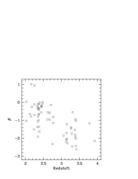
Figure 21: UV slope $\beta$ between 1200 and 1800 Å (Leitherer et al. LEI02 (2002)) as a function of redshift for the FDF galaxy subsample used in the calculation of the composite spectra (see Sect. 9.2). Typical errors of $\beta$ are around $0.1$.

Figure 22: UV slope $\beta$ as a function of the luminosities at 1500 Å for the FDF galaxy subsample used in the calculation of the composite spectra. Squares mark galaxies at $z<3$. Triangles indicate galaxies at $z>3$. Typical errors of $\beta$ are around $0.1$.

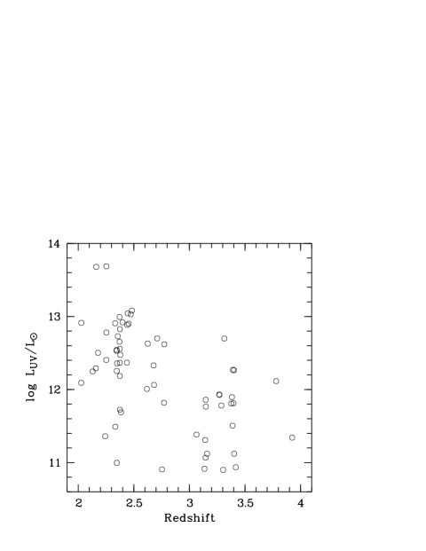
Figure 23: Total extinction-corrected UV luminosity in solar units as a function of redshift for the FDF galaxy subsample used in the calculation of the composite spectra.

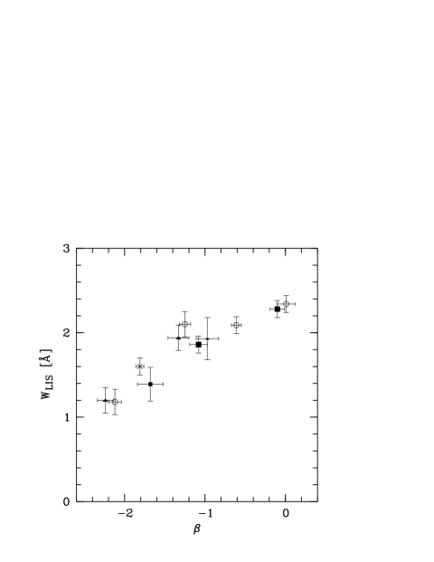
Figure 24: The dependence of the strength of low ionisation lines (see Fig. 16) on the continuum slope $\beta$. The open circles indicate values measured in FDF composite spectra representative of the different quartiles (containing 16 objects each) of the $\beta$ distribution derived from the individual spectra. The subsamples of the ranges $2<z<3$ (filled squares) and $3<z<4$ (filled triangles) were divided into two parts of equal number and averaged using $\beta$ as classification parameter. Data points representing the six steepest continua ($\beta<-1.3$) at $z<3$ and the five flattest continua ($\beta>-1.3$) at $z>3$ are marked by a small filled square and triangle, respectively. For comparison the corresponding data from S (03) are also shown (crosses).

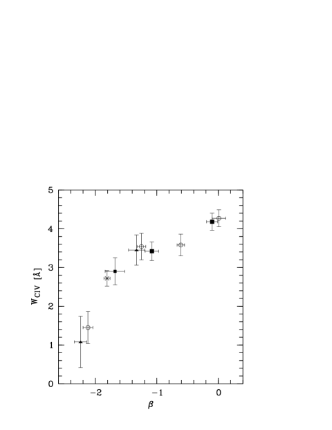
Figure 25: The dependence of the C IV equivalent width on the continuum slope parameter $\beta$. The data points were derived from composite spectra for different $\beta$ and $z$ intervals. Symbols are as in Fig. 24.

In principle, the UV continuum slope $\beta$ can be affected by various effects, such as the star-formation history (which determines the composition of the stellar population), the initial mass function, the chemical composition, dust extinction and the contribution of a possible AGN. However, for starburst galaxies showing a very young stellar population the predominant effect is expected to be dust reddening (see Calzetti et al. CAL94 (1994); Leitherer et al. LEI99 (1999), LEI02 (2002)). This implies that $\beta$ depends on the distribution of dust in the galaxy and on the metallicity (see Heckman et al. HEC98 (1998)), which has an important impact on the dust formation.

In Table 3 $\beta$ was found to be strongly redshift dependent, evolving from $\beta=-1.8$ at $z\sim 3.3$ to $\beta=-0.6$ at $z\sim 2.4$. To study this effect in more detail we also calculated the $\beta$ values of the individual galaxies. The resulting Fig. 21 confirms the change of $\beta$ with redshift.

To exclude that these results are due to a luminosity-related selection effect, we plotted in Fig. 22 $\beta$ as a function of the galaxy luminosity at 1500 Å (see Fig. 11). As shown by the figure, the $z>3$ objects show a distinctly higher average luminosity ($\langle\log L_{1500}[{\rm W/\AA}]\rangle=34.35\pm 0.04$ in comparison to $34.14\pm 0.03$ for the lower redshift range). This effect is mainly due to our selection criteria, causing an increase of the luminosity limit with increasing redshift. Thus, we cannot exclude the existence of reddened faint $z>3$ galaxies. On the other hand, the $z<3$ sample contains only a few ‘blue’ galaxies, although the brightness limits would allow their detection. Furthermore, a different sample selection would not increase the number of such galaxies significantly, since only a few luminous FDF objects have suitable magnitudes and colours. Finally, the $I$ magnitude based sample selection does not introduce a significant $\beta$-related selection effect. Assuming no evolution, the ratio of ‘blue’ to ’red’ galaxies should be almost the same for $z\sim 2.3$ and $z\sim 3.3$, since $I(z\sim 3.3)-I(z\sim 2.3)$ $\approx f(1800\,{\rm\AA})/f(2400\,{\rm\AA})$ is similar for both galaxy types (compare Type IV and V in Fig. 3). Consequently, the conspicuous difference between the mean $\beta$ of the $\log L_{1500}[{\rm W/\AA}]\geq 34.2$ objects ($\langle\beta\rangle=-0.58\pm 0.13$ for $z<3$ in comparison to $\langle\beta\rangle=-1.74\pm 0.13$ for $z>3$) is obviously real and cannot be explained by the selection procedure applied.

The very different continuum slopes for similar absolute brightnesses suggest that there is a strong evolution of the intrinsic UV luminosities of the galaxies. Hence, we estimated this quantity following Leitherer et al. (LEI02 (2002)). Taking

$$A_{1500}=2.19\,(\beta-\beta_{0})$$ (10)

($A_{1500}$ being the attenuation at 1500 Å in mag), $\beta_{0}=-2.5$ and

$$\log L_{\rm UV}=\log L_{1500}+0.4\,A_{1500}+3.2,$$ (11)

we obtained the values plotted in Fig. 23. As expected, there is a significant redshift dependence of the extinction-corrected total UV luminosity, leading to very luminous galaxies ($L_{\rm UV}>10^{12}\,{\rm L_{\sun}}$) at $z<3$, while such objects are rare at higher redshifts. The galaxies at $z<2.5$ with $L_{\rm UV}\sim 10^{13}\,{\rm L_{\sun}}$ are particularly interesting, since they are as bright as the most luminous star-forming galaxies known, implying star-formation rates of several $100\,{\rm M_{\sun}}/{\rm yr}$ and more. Fig. 23 can be explained in the sense that the masses of bright starbursts grow with cosmic age.

Next, we analysed the dependence of $\beta$ on other spectral properties. For this, we divided our sample of 64 galaxies into four equally-occupied $\beta$ intervals and constructed composite spectra. Further $\beta$-dependent mean spectra were calculated by halving the subsamples of the ranges $2<z<3$ and $3<z<4$ according to the continuum slope. The strong $\beta$ evolution made it necessary to construct composite spectra including the six steepest spectra ($\beta<-1.3$) with $z<3$ and the five flattest ones ($\beta>-1.3$) with $z>3$, respectively.

In Fig. 24 we show the average EW of the six strong low-ionisation lines (see Fig. 16) as a function of $\beta$. The figure indicates a monotonic relation, characterised by a decrease of $W_{\rm LIS}$ with bluer continua. A slight redshift dependence of the relation cannot be excluded, since $W_{\rm LIS}$ seems to be smaller at constant $\beta$ towards lower redshifts. Heckman et al. (HEC98 (1998)) conjecture that the $W_{\rm LIS}-\beta$ relation could be caused by a relation between dust extinction and turbulent velocity of the interstellar medium. This could be due to the dustier galaxies being more massive and showing stronger and more violent star-formation. According to S (03) the $W_{\rm LIS}-\beta$ relation may be due to the change of the covering fraction of the hot stars by interstellar clouds consisting of neutral gas and dust, which gives a more direct link between both quantities than the former explanation.

Fig. 25 indicates a relatively tight relation between $W_{\rm C\,IV}$ and $\beta$, which does not show a redshift evolution. In part the strong decrease of $W_{\rm C\,IV}$ with $\beta$ for $\beta<-1.5$ can be due to a C IV emission component. Fig. 25 supports the assumption that the dust reddening depends partly on the metallicity, which is traced by C IV (see Heckman et al. HEC98 (1998); Leitherer et al. LEI01 (2001); Mehlert et al. MEH02 (2002)).

10 Implications and conclusions

As described in the preceding sections, in addition to providing valuable information on the spectral properties of distant galaxies, the FDF spectroscopic survey also provided interesting new data on the evolution of the properties of bright starburst galaxies $2<z<5$. The main results on this redshift evolution can be summarised as follows:

• Although the spectra of the starburst galaxies are basically very similar at all observed redshifts, there is a tendency for the net line absorption to become weaker with increasing redshift. In particular, our galaxy spectra with $z>3$ show on average weaker absorption and/or stronger emission components. The effect is particularly conspicuous for the Ly$\alpha$ line and the C IV resonance doublet.

• The UV continuum slope tends to become flatter with decreasing redshift. Since for bright starburst galaxies this slope is mainly determined by the internal reddening, this correlation also indicates an increase of dust reddening with cosmic age.

• Our data show an anticorrelation of low-ionisation interstellar absorption lines with the Ly$\alpha$ emission strength (reported already by S (03)) and a positive correlation of these lines with the reddening. These correlations do not show a significant redshift dependence.

• The C IV absorption strength (while clearly dependent on the redshift) shows only little correlation with the Ly$\alpha$ emission or absorption strength. On the other hand, a positive, redshift-independent correlation between the C IV absorption strength and the dust reddening was found.

• The anticorrelation between the reddening and the Ly$\alpha$ emission strength shows a striking redshift dependence, at least for absorption-dominated Ly$\alpha$ profiles, where the average UV continuum flattens with decreasing redshift.

• Although our flux-limited spectroscopic sample is observationally biased towards absolutely brighter objects at higher redshifts, the average intrinsic UV luminosity of the starburst galaxies in our sample decreases with redshift for $2<z<4$.

As shown by Mehlert et al. (MEH02 (2002)) the increase of the C IV absorption strength with decreasing redshift can be readily explained by the cosmic heavy element enrichment history of starburst galaxies in an evolving universe. The cosmic chemical evolution also provides a plausible explanation for the observed dependence of the UV continuum slope $\beta$ and the Ly$\alpha$ emission strength on the redshift. For a lower metallicity we expect a lower dust content (and consequently a lower reddening), a higher escape probability for Ly$\alpha$ photons, and higher temperatures of the radiation field and gas of the starburst galaxies. This prediction is in good agreement with the observed steeper continuum slope and (on average) larger Ly$\alpha$ emission observed for $z>3$.

On the other hand, the Ly$\alpha$ emission shows a relatively strong correlation with the low-ionisation absorption lines as compared to the relatively poor correlation with the C IV absorption. Since $W_{\rm LIS}$ traces the properties of (dusty) interstellar H I clouds (see S (03)), a strong influence of the velocity field and/or the geometric structure of the interstellar medium (and resulting covering fractions) on the observed Ly$\alpha$ flux and its evolution can be assumed. The observational result that a significant fraction of the galaxies with $z>3$ show Ly$\alpha$ in absorption, although the average reddening is distinctly lower than for the corresponding $2<z<3$ galaxies, could also be explained by an evolution of the properties of the interstellar medium.

The decrease of the average Ly$\alpha$ emission and the conspicuous enhancement of the dust reddening with decreasing redshift may be partly due to an increase of the average cold gas and dust mass of the galaxies, which impedes the escape of UV photons from the galaxy by an enhanced obscuration of the luminous hot stars and H II regions in the starburst cores. Assuming that the intrinsic UV luminosities of the high-redshift galaxies are characteristic for their starburst mass, the observed increase of the mean absolute luminosity with decreasing redshift of the galaxies in our $2<z<4$ sample suggests mass evolution as well. This result can be interpreted within current hierarchical models for the formation and evolution of galaxies.

Summarising, we conclude that the observed evolution with redshift of the basic properties of the galaxies in the FDF spectroscopic survey sample can be well explained on the basis of present theoretical concepts and theories of the formation and chemical evolution of galaxies. Hence, the data described in this paper provide strong further support for these theoretical concepts and models as well as a potential basis for additional investigations of the details of such models.

- (1) Adelberger, K.L., Steidel, C.C., Giavalisco, M., er al. 1998, ApJ, 505, 18
- (2) Adelberger, K.L., Steidel, C.C., Shapley, A.E., et al. 2003, ApJ, 584, 45
- (3) Appenzeller, I., Bender, R., Böhm, A., et al. 2000, The Messenger, 100, 44
- (4) Bender, R., Appenzeller, I., Böhm, A., et al. 2001, in Deep Fields, ed. S. Cristiani, A. Renzini, & R.E. Williams, ESO astrophysics symposia (Springer), 96
- (5) Bender, R., et al. 2004, in preparation
- (6) Böhm, A., Ziegler, B.L., Saglia, R.P., et al. 2004, A&A, accepted (astro-ph/0309263)
- (7) Calzetti, D., Kinney, A.L., & Storchi-Bergmann, T. 1994, ApJ, 429, 582
- (8) Cardelli, J.A., Clayton, G.C., & Mathis J.S. 1989, ApJ, 345, 245
- (9) Charlot, S., & Fall, M.S. 1993, ApJ, 415, 580
- (10) Cohen, J.G., Hogg, D.W., Blandford, R., et al. 2000, ApJ, 538, 29
- (11) Connolly, A.J., Szalay, A.S., Dickinson, M., et al. 1997, ApJ, 486, L11
- (12) Cowie, L.L., & Hu, E.M. 1998, AJ, 115, 1319
- (13) Cristiani, S., Appenzeller, I., Arnouts, S., et al. 2000, A&A, 359, 489
- (14) Daddi, E., Cimatti, A., Renzini, A., et al. 2004, ApJ, 600, L127
- (15) Ferguson, H.C., Dickinson, M., & Williams, R. 2000, ARA&A, 38, 667
- (16) Ferguson, H.C., Dickinson, M., Giavalisco, M., et al. 2004, ApJ, 600, L107
- (17) Fernández-Soto, A., Lanzetta, K.M., & Yahol, A. 1999, ApJ, 513, 34
- (18) Frank, S., Appenzeller, I., Noll, S., et al. 2003, A&A, 407, 473
- (19) Frye, B., Broadhurst, T., & Benítez, N. 2002, ApJ, 568, 558
- (20) Gabasch, A., Bender, R., Hopp, U., et al. 2004, A&A, submitted
- (21) Giavalisco, M. 2002, ARA&A, 40, 579
- (22) Hamuy, M., Walker, A.R., Suntzeff, N.B., et al. 1992, PASP, 104, 533
- (23) Hamuy, M., Suntzeff, N.B., Heathcote, S.R., et al. 1994, PASP, 106, 566
- (24) Heckman, T.M., Robert, C., Leitherer, C., et al. 1998, ApJ, 503, 646
- (25) Heidt, J., Appenzeller, I., Noll, S., et al. 2003a, Carnegie Observatory Astrophysics Series, Vol.1: Coevolution of Black Holes and Galaxies, ed. L.C. Ho (Pasadena: Carnegie Observatories, http://www.ociw.edu/ociw/ symposia/series/symposium1/proceedings.html)
- (26) Heidt, J., Appenzeller, I., Gabasch, A., et al. 2003b, A&A, 398, 49
- (27) Horne, K. 1986, PASP, 98, 609
- (28) Hu, E.M., & McMahon, R.G. 1996, Nat, 382, 231
- (29) Hu, E.M., McMahon, R.G., & Cowie, L.L. 1999, ApJ, 522, L9
- (30) Hu, E.M., Cowie, L.L., Mc Mahon, R.G., et al. 2002, ApJ, 568, L75
- (31) Idzi, R., Sommerville, R., Papovich, C., et al. 2004, ApJ, 600, L115
- (32) Keenan, P.C., & Mc Neil, R.C. 1976, An atlas of spectra of the cooler stars: types G, K, M, S, and C, Columbus, Ohio State University Press
- (33) Kennicutt, R.C. Jr. 1992, ApJS, 79, 255
- (34) Kinney, A.L., Bohlin, R.C., Calzetti, D., et al. 1993, ApJS, 86, 5
- (35) Kinney, A.L., Calzetti, D., Bohlin, R.C., et al. 1996, ApJ, 467, 38
- (36) Kunth, D., Mas-Hesse, J.M., Terlevich, E., et al. 1998, A&A, 334, 11
- (37) Leitherer, C., Schaerer, D., Goldader, J.D., et al. 1999, ApJS, 123, 3
- (38) Leitherer, C., Leão, J.R.S., Heckman, T.M., et al. 2001, ApJ, 550, 724
- (39) Leitherer, C., Li, I.-H., Calzetti, D., et al. 2002, ApJS, 140, 303
- (40) Lehnert, M.D., & Bremer, M. 2003, ApJ, 593, 630
- (41) Lowenthal, J.D., Koo, D.C., Guzman, R., et al. 1997, ApJ, 481, 673
- (42) Madau, P., Pozzetti, L., & Dickinson, M. 1998, ApJ, 498, 106
- (43) Maier, C., Meisenheimer, K., Thommes, E., et al. 2003, A&A, 402, 79
- (44) Maraston, C. 1998, MNRAS, 300, 872
- (45) Martín, E.L., Delfosse, X., Basri, G., et al. 1999, AJ, 118, 2466
- (46) Mehlert, D., Seitz, S., Saglia, R.P., et al. 2001, A&A, 379, 96
- (47) Mehlert, D., Noll, S., Appenzeller, I., et al. 2002, A&A, 393, 809
- (48) Menou, K., Vanden Berk, D.E., Željko, I., et al. 2001, ApJ, 561, 645
- (49) Morgan, W.W., & Keenan, P.C. 1973, ARA&A, 11, 29
- (50) Oke, J.B. 1990, AJ, 99, 1621
- (51) Pettini, M., Steidel, C.C., Adelberger, K.L., et al. 2000, ApJ, 528, 96
- (52) Pettini, M., Rix, S.A., Steidel, C.C., et al. 2002, ApJ, 569, 742
- (53) Pickles, A.J. 1985, ApJS, 59, 33
- (54) Rhoads, J.E., Dey, A., Malhotra, S., et al. 2003, AJ, 125, 1006
- (55) Savaglio, S., Glazebrook, K., Abraham, R.G., et al. 2004 (astro-ph/0310437)
- (56) Schaerer, D. 2003, A&A, 397, 527
- (57) Schlegel, D.J., Finkbeiner, D.P., & Davis, M. 1998, ApJ, 500, 525
- (58) Shapley, A.E., Steidel, C.C., Adelberger, K.L., et al. 2001, ApJ, 562, 95
- S (03) Shapley, A.E., Steidel, C.C., Pettini, M., et al. 2003, ApJ, 588, 65 (S03)
- (60) Simkin, S.M. 1974, A&A, 31, 129
- (61) Spinrad, H., Stern, D., Bunker, A., et al. 1998, AJ, 116, 2617
- (62) Steidel, C.C., Giavalisco, M., Pettini, M., et al. 1996a, ApJ, 462, L 17
- (63) Steidel, C.C., Giavalisco, M., Dickinson, M., et al. 1996b, AJ, 112, 352
- (64) Steidel, C.C., Adelberger, K.L., Dickinson, M., et al. 1998, ApJ, 492, 428
- (65) Steidel, C.C., Adelberger, K.L., Giavalisco, M., et al. 1999, ApJ, 519, 1
- (66) Steidel, C.C., Pettini, M., & Adelberger, K.L. 2001, ApJ, 546, 665
- (67) Steidel, C.C., Adelberger, K.L., Shapley, A.E., et al. 2003, ApJ, 592, 728
- (68) Tapken, C., Appenzeller, I., Mehlert, D., et al. 2003, A&A, in press (astro-ph/0401419)
- (69) Tonry, J., & Davis, M. 1979, AJ, 84, 1511
- (70) Tüg, H., 1977, The Messenger, 11, 7
- (71) Vanzella, E., Cristiani, S., Arnouts, S., et al. 2002, A&A, 396, 847
- (72) Walborn, N.R., Lennon, D.J., Haser, S.M., et al. 1995, PASP, 107, 104
- (73) Weymann, R.J., Stern, D., Bunker, A., et al. 1998, ApJ, 505, 95
- (74) Williams, R.E., Blacker, B., Dickinson, M., et al. 1996, AJ, 112, 1335
- (75) Ziegler, B.L., Boehm, A., Fricke, K.J., et al. 2002, ApJ, 564, L69
- (76) Ziegler, B.L., Thomas, D., Böhm, A., et al. 2004, in preparation