Water Absorption From Line-of-Sight Clouds Toward W49A

Abstract

We have observed 6 clouds along the line-of-sight toward W49A using the Submillimeter Wave Astronomy Satellite (SWAS) and several ground-based observatories. The ortho-H₂O $1_{10}\rightarrow 1_{01}$ and OH (1665 and 1667 MHz) transitions are observed in absorption, whereas the low-J CO, ¹³CO, and C¹⁸O lines, as well as the [C I] ${}^{3}P_{1}-^{3}P_{0}$ transition, are seen in emission. The emission lines allow us to determine the gas density (n $\sim 1500-3000$ cm^-3) and CO column densities ($N(CO)\sim 7.9\times 10^{15}-2.8\times 10^{17}$ cm^-2) using a standard Large Velocity Gradient analysis.

By using both the o-H${}_{2}^{18}$O and o-H₂O absorption lines, we are able to constrain the column-averaged o-H₂O abundances in each line-of-sight cloud to within about an order of magnitude. Assuming the standard N(H₂)/N(CO) ratio of $10^{4}$, we find N(o-H₂O)/N(H₂) = $8.1\times 10^{-8}-4\times 10^{-7}$ for three clouds with optically thin water lines. In three additional clouds, the H₂O lines are saturated so we have used observations of the H${}_{2}^{18}$O ground-state transition to find upper limits to the water abundance of $8.2\times 10^{-8}-1.5\times 10^{-6}$. We measure the OH abundance from the average of the 1665 and 1667 MHz observations and find N(OH)/N(H₂) = $2.3\times 10^{-7}-1.1\times 10^{-6}$. The o-H₂O and OH abundances are similar to those determined for line-of-sight water absorption features towards W51 and Sgr B2 but are higher than those seen from water emission lines in molecular clouds. However, the clouds towards W49 have lower ratios of OH relative to H₂O column densities than are predicted by simple models which assume that dissociative recombination is the primary formation pathway for OH and H₂O. Building on the work of Neufeld et al. (2002), we present photo-chemistry models including additional chemical effects, which can also explain the observed OH and H₂O column densities as well as the observed H₂O/CO abundance ratios.

1 Introduction

Since its launch in 1998 December, the Submillimeter Wave Astronomy Satellite (SWAS) has observed emission from the ground-state ($1_{10}\rightarrow 1_{01}$) transition of ortho-H₂O (hereafter o-H₂O) in a number of molecular clouds (e.g. Melnick et al. 2000a; Snell et al. 2000a, 2000b). While it has been possible to determine the H₂O abundances from the SWAS observations, these analyses depend on the often poorly contrained gas densities and temperatures. Observations of absorption from the o-H₂O ground-state transition, however, have the advantage that the column density is simply proportional to the optical depth in the line. Therefore, the H₂O abundance can be derived without precise knowledge of the temperature or density of the absorbing gas.

In this paper we present observations of water absorption toward the molecular cloud complex W49A. W49 is 11.4 kpc from the Sun and 8.1 kpc from the Galactic Center (Gwinn et al. 1992). It consists of a supernova remnant (W49B) and an HII region (W49A) separated by $\sim 12^{\prime}$. W49A has long been known as a site of extremely active star formation, due to its association with one of the most powerful H₂O masers in the Galaxy (Genzel et al. 1978), and the fact that it is one of the most luminous regions in the Galaxy ($L_{bol}\sim 10^{7}$ L_⊙; Ward-Thompson & Robson 1990). Physically, W49A is composed of a number of optically obscured, compact HII regions surrounded by a massive molecular cloud ($M>10^{5}$ M_⊙; Mufson & Liszt 1977). W49A is broken up into three main IR peaks; W49SW, W49SE and, the strongest, W49NW (more commonly named W49N; Harvey et al. 1977). The continuum emission from W49A has also been observed at 350, 800, and 1100 $\mu$m by Ward-Thompson and Robson (1990) and at 1300 $\mu$m by Schloerb et al. (1987).

Spectrally, W49A is extremely complex, containing numerous features contributed by W49A itself, as well as additional clouds associated with the Sagittarius spiral arm (which crosses the line-of-sight twice). W49A and the associated line-of-sight clouds have been the subject of numerous spectroscopic studies (both emission and absorption) involving species such as HI (Radhakrishnan et al. 1972), HCO⁺ and HCN (Nyman 1983), OH (Cohen and Willson 1981), H₂CO (Mufson and Liszt 1977; Bieging et al. 1982), CO (Mufson and Liszt 1977), SiO (Lucas and Liszt 2000), CS (Greaves and Williams 1994), and OI (Vastel et al. 2000).

The strong continuum provided by this source, and the well-studied deep absorption features in the gas associated with line-of-sight clouds, provide an excellent opportunity to measure the H₂O abundances in a number of different molecular clouds. Similar analyses of the water abundances have recently been carried out for line-of sight clouds toward Sagittarius B2 ( Neufeld et al. 2000; Cernicharo et al. 1997), Sagittarius A* (Moneti et al. 2001), and W51 (Neufeld et al. 2002).

2 Observations

Since SWAS has two independent receivers, we were able to simultaneously observe the [C I] ${}^{3}P_{1}\rightarrow^{3}P_{0}$ ($\nu=492.1607$ GHz) and O₂ $3,1\rightarrow 3,2$ ($\nu=487.249$ GHz) transitions in the upper and lower sidebands of receiver 1, and the ¹³CO  $J=5\rightarrow 4$ ($\nu=550.926$ GHz) and o-H₂O $1_{10}\rightarrow 1_{01}$ ($\nu=556.936$ GHz) transitions in the upper and lower sidebands of receiver 2. However, when receiver 2 was tuned to the o-H${}_{2}^{18}$O $1_{10}\rightarrow 1_{01}$ transition ($\nu=547.676$ GHz), SWAS loses the ability to observe o-H₂O and ¹³CO $J=5\rightarrow 4$. The integration times and $1\sigma$ rms noise levels for each line are listed in Table 1. The SWAS beamsize at 557 GHz is $3.3^{\prime}\times 4.5^{\prime}$ while at 490 GHz it is $3.5^{\prime}\times 5.0^{\prime}$. The main beam efficiency ($\eta_{mb}$) for SWAS is 90%. For more information about the SWAS instrument, data acquisition, and data analysis, see Melnick et al. (2000b).

The SWAS observations of W49 were obtained in four different observing periods; 1999 April and May, 1999 September and October, 2000 March - May, and 2000 October. The central position (located at W49N) is given as $\alpha(J2000)=19^{h}10^{m}13.5^{s}$, $\delta(J2000)=09^{\circ}:06^{\prime}:29^{\prime\prime}$. The reference position was $\sim 1.5^{\circ}$ from the central position ($\alpha(J2000)=19^{h}15^{m}19.8^{s}$, $\delta(J2000)=08^{\circ}:15^{\prime}:22^{\prime\prime}$) and was chosen based on an absence of ¹²CO  $J=1\rightarrow 0$ emission.

In order to understand the H₂O and OH absorption, it is important to know the spatial extent of the submillimeter continuum. To this end, we have mapped a region in W49 comparable to the SWAS beam at 450 $\mu$m using the SHARC camera at the Caltech Submillimeter Observatory (CSO). These observations were taken in 1999 September. The flux levels were calibrated using Uranus as the calibration source. In addition to the SHARC maps, we also have data from the on-board SWAS continuum detectors in the fast-chop (4 Hz) observing mode (see Melnick et al. 2000b for details).

We observed ¹²CO $J=1\rightarrow 0$ ($\nu=115.271$ GHz), ¹³CO $J=1\rightarrow 0$ ($\nu=110.201$ GHz), and C¹⁸O  $J=1\rightarrow 0$ ($\nu=109.782$ GHz), at the 14m Five Colleges Radio Astronomy Observatory (FCRAO) using their 32 element array receiver (SEQUOIA). The ¹²CO  $J=1\rightarrow 0$ observations were taken in 2001 August on an 8 beam $\times$ 8 beam grid with 44^′′ spacings (the resolution of the FCRAO antenna). The ¹³CO and C¹⁸O  $J=1\rightarrow 0$ observations were obtained in 2002 November. For comparison with the SWAS H₂O observations these data were smoothed to a resolution of 1.5^′ to match the size of the continuum source in W49 (see Section 3.1). The main beam efficiency ($\eta_{mb}$) of the FCRAO is 49%

Observations of the ¹²CO  $J=3\rightarrow 2$ transition were made at the KOSMA (Kölner Observatorium für Submm-Astronomie) 3m telescope near Zermatt, Switzerland. The observations were taken on 2000 November 19 using the MRS (medium resolution acousto optical spectrometer) backend with a resolution of 360 kHz, corresponding to 0.31 km s^-1 at 345 GHz. The beamsize at 345 GHz is 82^′′ and the main beam efficiency ($\eta_{mb}$) is 78%. For comparison with the SWAS observations, these data were smoothed to match the spatial resolution of the SWAS ¹³CO  $J=5\rightarrow 4$ observations.

In order to further examine the line-of-sight clouds towards W49A, observations of the F = $1\rightarrow 1$ (1665 MHz) and F = $2\rightarrow 2$ (1667 MHz) transitions of OH were obtained at the Arecibo Observatory in 2001 December. At these frequencies, the Arecibo beam size is approximately $2.6^{\prime}\times 3^{\prime}$ (FWHM) and has a main beam efficiency at 1665 & 1667 MHz of 80%. We also obtained observations of the 1612 and 1720 MHz transitions of OH at the Arecibo observatory in 2003 October allowing us to investigate LTE versus non-LTE excitation in the OH lines,

The on-source integration times and 1 $\sigma$ rms noise levels for each of the observed spectral lines are presented in Table 1. All spectra in this paper are presented in units of T${}_{A}^{*}$. For subsequent analysis we use the main beam temperature (T_mb) which is defined by the standard equation T${}_{mb}=T_{A}^{*}/\eta_{mb}$ where $\eta_{mb}$ is the main beam efficiency.

3 Results

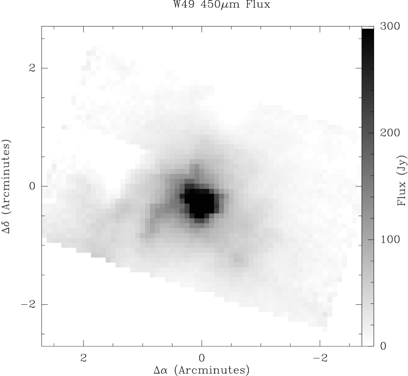
Figure 1: 450 $\mu$m continuum emission from W49A from SHARC at the CSO with a beamsize of approximately 9^′′. The peak flux is $\sim$ 700 Jy but the image scale is truncated at 300 Jy to better show the weak, extended emission.

Figure 1 shows the 450 $\mu m$ continuum emission obtained using SHARC at the CSO. The continuum emission is strongly concentrated on W49A itself but with weaker tendrils of emission extended approximately $0.75^{\prime}$ from the center. We use the 450 $\mu$m map of W49 to confirm the continuum level in the SWAS o-H₂O and o-H${}_{2}^{18}$O spectra. First, we extrapolate the integrated 450 $\mu$m continuum emission to 540 $\mu$m (the wavelength of the SWAS o-H₂O line) assuming a power law of the form $S\propto\lambda^{-3.5}$. Then, we convert the integrated flux at 540 $\mu$m to an equivalent main beam brightness temperature (T_mb) through the standard equation: $S={{2kT_{mb}\Omega}\over{\lambda^{2}}}$. Using parameters appropriate for the SWAS beam at 540 $\mu$m, we obtain $T_{mb}\sim S(Jy)/13982$. The integrated fluxes for W49 are 1827 Jy at 450 $\mu$m and 965 Jy at 540 $\mu$m, corresponding to T_mb = 0.07 K at 540 $\mu$m.

At 539 $\mu$m, the SWAS on-board continuum detectors yield a T_mb of 0.1 K for W49A. The fact that the SWAS results are $\sim$ 30% higher than SHARC observations probably reflects uncertainties in the extrapolation to 540 $\mu$m, atmospheric effects, and the fact that the SHARC maps do not perfectly match the SWAS beam size, shape, and orientation. It should be noted, however, that the SWAS measurements may not be entirely accurate, due to a relatively slow chop rate. Therefore, for the subsequent analysis in this paper we instead use the fact that four of the H₂O absorption features are at the same depth to within the noise (the $\sim 18$ km s^-1 component from W49 itself, and the 39.5, 59.6, and 63.3 km s^-1 features; see Figure 2). This strongly suggests that these lines are saturated and thus, the continuum flux level can be set by the depth of these four features. The average depth of these four lines is 0.08 K ($T_{A}^{*}$) which agrees satisfactorily with both our measurement from SWAS’ on-board continuum detectors and our extrapolation of the SHARC data.

Figure 2 shows the o-H₂O $1_{10}\rightarrow 1_{01}$, [C I] ${}^{3}P_{1}\rightarrow^{3}P_{0}$, and ¹³CO  $J=5\rightarrow 4$ observations from SWAS. Velocities less than $\sim 30$ km s^-1 correspond to emission/absorption intrinsic to W49A and these features are not further analysed in this paper. At velocities greater than $\sim 30$ km s^-1, Figure 2 shows six distinct o-H₂O absorption dips at LSR velocities of 33.5, 39.5, 53.5, 59.6, 63.3 and 68 km s^-1. Gaussian fits to the baseline subtracted spectra are listed in Table 2 for each of the water absorption features. The same six features are seen in emission in the [C I] spectrum (Figure 2), although at slightly different LSR velocities. The slight offset between the [C I] and o-H₂O line centers may be partly due to the high optical depths of the water lines. The Gaussian fits to the baseline subtracted carbon lines are given in Table 3. No ¹³CO $J=5\rightarrow 4$ lines were detected at velocities $>30$ km s^-1. The O₂ transition was not detected to a $3\sigma$ level of 15 mK.

Figure 3 shows the ¹²CO, ¹³CO and C¹⁸O  $J=1\rightarrow 0$ observations from FCRAO and the ¹²CO  $J=3\rightarrow 2$ observations from KOSMA. All spectra have been convolved to a circular, Gaussian beam of $3.8^{\prime}$ to match the beam resolution of the SWAS ¹³CO $J=5\rightarrow 4$ observations . Figure 3 shows that while all six H₂O absorption features are seen in both CO lines and the ¹³CO  $J=1\rightarrow 0$ lines, the less abundant C¹⁸O  $J=1\rightarrow 0$ only shows the 3 strongest components. It should be noted that, while the spectra in Figure 3 have been smoothed to match the spatial resolution of the SWAS beam, for our subsequent LVG analysis (Section 3.1), we use data smoothed to the size of the background continuum source (1.5^′). Since we are trying to estimate the CO column density in the gas which is absorbing the H₂O, it is more relevant to coadd only those ¹³CO and C¹⁸O spectra that fall in front of the continuum source. Therefore, we coadd the ¹³CO and C¹⁸O spectra within $\sim 0.75^{\prime}$ of the central position (Figure 1). Gaussian fits to the detected spectral features in the data smoothed to 1.5^′ (with first order baselines subtracted) are given in Table 4.

Figure 4 plots the line to continuum flux ratio for the SWAS observations of both o-H₂O and o-H${}_{2}^{18}$O. The line to continuum flux ratio is given by $F_{l}/F_{c}=[\Delta T_{mb}(line)+T_{mb}(cont)]/T_{mb}(cont)$ where $T_{mb}(cont)$ is the measured main beam, SSB continuum flux level (see above) and $\Delta T_{mb}(line)$ is the baseline subtracted antenna temperature ($\Delta T_{A}^{*}$; listed in Table 2) divided by the main beam efficiency. Although there are no clear o-H${}_{2}^{18}$O lines at velocities $>30$ km s^-1, we provide upper limits in Table 2 by fitting Gaussians with $LSR$ velocities and $FWHM$ linewidths fixed at the values provided by the [C I] emission lines. We used the [C I] spectrum as a template, rather than the o-H₂O spectrum, due to the large optical depths of the water line. Therefore, Table 2 provides limits to the o-H${}_{2}^{18}$O line strengths and integrated intensities. Table 2 also lists the line to continuum flux ratios (seen in Figure 4) and the line center optical depth ($\tau_{o}=-ln(F_{l}/F_{c})$).

Since the continuum level is set by the average depth of the four deepest absorption features, the 39.5, 59.6, and 63.3 km s^-1 o-H₂O features in Figure 4 reach line-to-continuum values close to, or less than, zero (and are, in fact, as strong as the absorption feature associated with W49A itself). Therefore, these features are most likely saturated, and we would consequently derive a null or negative line flux and an unphysical opacity. For these three lines, we provide a minimum line center opacity in Table 2 by adding the $1\sigma$ error of the Gaussian fits ( $T_{A}^{*}$ = 0.006 K) to the measured continuum level. The other three features (at 33.5, 53.5, and 68 km s^-1) are weaker and appear optically thin. It is important to note however, that while we assume these components to be optically thin they may, in fact, have a higher optical depth. The relative line strengths of the six ¹³CO  $J=1\rightarrow 0$ components show significant variation over the region mapped, implying the presence of cloud structure on scales smaller than the SWAS beam. Therefore, we cannot rule out the possibility that the 33.5, 53.5, and 68 km s^-1 features are actually saturated and only appear to be optically thin because they do not completely cover the continuum source. Nevertheless, for the subsequent analysis in this paper we will assume that these three components are unsaturated.

Figure 5 plots the line to continuum flux ratio for the Arecibo observations of the OH 1665 MHz and 1667 MHz transitions. Since the front end amplifiers at the Arecibo observatory have uniquely defined pass bands, there is no single sideband to double sideband conversion issue. Thus, the measured SSB continuum levels ($T_{mb}(cont)$) are 311.3 K at 1665 MHz and 315.3 K at 1667 MHz. All six of the features seen in emission in [CI] are seen in absorption in both OH lines. Table 5 lists the Gaussian fit parameters to all six components (with a first order baseline removed), as well as the line to continuum flux ratios and associated line center optical depth. The lines at 39.3, 54.2, 62.9, and 68.8 km s^-1 are all within 25% of the 5/9 integrated intensity ratio expected for the 1665/1667 lines in local thermodynamic equilibrium (LTE). The 1665/1667 ratios in the 33.6 and 59.8 km s^-1 lines, however, are $\sim 1/3$ which is $\sim 40$% lower than expected for LTE. The weakness of these lines suggests that they are optically thin. Therefore, the 1665/1667 ratio of 1/3 seen in the 33.6 and 59.8 km s^-1 lines is probably a result of non-LTE excitation and not a line saturation effect. In addition, our most recent OH observations (at 1612, 1665, 1667, and 1720 MHz) taken at the Arecibo observatory strongly suggest that the 39.3 and 62.9 km s^-1 features are also affected by non-LTE excitation. Therefore, we will restrict further analysis of the OH absorption lines to the 54.2 and 68.8 km s^-1 components.

3.1 CO and C^o Abundances

To determine the line-of-sight average H₂O and OH abundances, we first need to estimate the CO column density corresponding to each of the six water absorption features. To do this, we use a Large Velocity Gradient (LVG) code to simultaneously fit the ¹³CO  $J=1\rightarrow 0$, $5\rightarrow 4$, and C¹⁸O  J = $1\rightarrow 0$ observations. Since ¹³CO  $J=5\rightarrow 4$ emission was not detected in any of the clouds, we use the 1 $\sigma$ noise level in the spectrum as an upper limit to the line strength in order to better constrain the fitting routine. We do not include the ¹²CO observations in this analysis due to the higher opacity in these transitions and chose to focus instead on the optically thin tracers. An investigation into the effect of ignoring the ¹²CO data in the LVG fits shows that the derived densities and column densities change by less than a factor of 2. We also use the data listed in Table 4, which have been smoothed to the size of the background continuum source rather than to the spatial resolution of the SWAS beam. The densities and column densities determined from this data set, however, do not differ significantly from an identical analysis using data coadded over an entire SWAS beam.

We created a $20\times 20$ grid of models in density-column density parameter space using a constant kinetic temperature of 8 K (Vastel et al. 2000), consistent with what is derived from our ¹²CO observations assuming that the emission is optically thick and thermalized. The densities range from $1000-5000$ cm^-3 and the ¹³CO column densities (per velocity interval) range from $10^{13}-10^{16}$ cm^-2/km s^-1. To fit the observations of the ¹³CO and C¹⁸O isotopologues we assume isotopic abundance ratios (with respect to CO) of 55 and 500 respectively. The observed line intensities are fit to the grid of LVG models using a $\chi^{2}$ minimization routine to find the density and column density combination that best fit the observations. Results from the LVG fitting are listed in Table 6 along with the estimated visual extinctions where we have assumed that N(H₂) $\sim 8\times 10^{20}A_{V}$ and N(H₂)/N(CO) $\sim 10^{4}$. It is important to note that this only estimates the dust extinction in the CO emitting region and ignores any additional extinction which may arise in overlying layers of HI or H₂. To check the sensitivity of our results to our assumed value of kinetic temperature, we performed an identical LVG analysis using kinetic temperature of 15 K instead of 8 K. The resultant densities change by less than a factor of three and the column densities by less than 25%.

Using the H₂ density in Table 6 we also calculate the neutral carbon (C^o) column density from the SWAS [C I] ${}^{3}P_{1}\rightarrow^{3}P_{0}$ observations (using the same LVG code and again assuming a kinetic temperature of 8 K). The results are also tabulated in Table 6 along with the C^o/CO abundance ratio. The C^o/CO abundance ratio varies from 0.6 for clouds with inferred visual extinctions (A_V) of 1.9, to C^o/CO = 3.8 for clouds with inferred A_V = 0.1. These numbers are consistent with C^o/CO ratios seen at the low column density edges of UV illuminated giant molecular clouds (e.g. Plume et al 1999) and with previous observations of high-latitude and translucent clouds (Ingalls et al 1997; Stark et al 1996; Stark & van Dishoeck 1994).

3.2 H₂O and OH Abundances

The SWAS ortho-H₂O column densities are derived from a “curve of growth” analysis of SWAS o-H${}_{2}^{18}$O and o-H₂O spectra. The column density in the lower state ($N_{l}$)can be expressed as:

$$N_{l}={{g_{l}}\over{g_{u}}}{{8\pi\nu_{o}^{3}}\over{c^{3}}}{{\sqrt{\pi}}\over{A_{ul}}}{{1}\over{[1-e^{-h\nu/kT_{ex}}]}}\tau_{o}{{\Delta V(FWHM)}\over{2\sqrt{ln2}}},~{}~{}~{}~{}~{}~{}(1)$$

where $\tau_{o}$ is the optical depth at line center. For the o-H₂O and o-H${}_{2}^{18}$O absorption lines in W49, T_ex is probably much less than $h\nu/k$ = 27 K, and so equation (1) reduces to:

$$N_{l}={{g_{l}}\over{g_{u}}}{{8\pi}\over{\lambda_{o}^{3}}}{{\sqrt{\pi}}\over{A_{ul}}}~{}~{}\tau_{o}{{\Delta V(FWHM)}\over{2\sqrt{ln2}}}.~{}~{}~{}~{}~{}~{}(2)$$

Using parameters appropriate for the SWAS observations: $\lambda(o-H_{2}^{18}O)=547.39\mu m$, $\lambda(o-H_{2}O)=538.66\mu m$, $A_{ul}=3.5\times 10^{-3}$ s^-1 (for both o-H₂O and o-H${}_{2}^{18}$O), and $g_{l}/g_{u}=1$, the expressions for the column density reduce to:

$$N_{l}(o-H_{2}^{18}O)=4.66\times 10^{12}~{}~{}\tau_{o}(H_{2}^{18}O)\Delta V(FWHM),~{}~{}~{}~{}~{}(3)$$

and

$$N_{l}(o-H_{2}O)=4.89\times 10^{12}~{}~{}\tau_{o}(H_{2}O)\Delta V(FWHM),~{}~{}~{}~{}~{}(4)$$

where $\Delta V(FWHM)$ is in units of km s^-1. Again, since the excitation temperatures in these clouds is low, $N_{l}$ is, to first approximation, equal to the total column density. $\tau_{o}$ is the line center optical depth of the particular molecular transition.

Table 7 presents the ortho-water column density in each of the six line-of-sight absorption features towards W49A. The first row lists upper limits on $\tau_{o}\Delta V$ for o-H${}_{2}^{18}$O taken from the o-H${}_{2}^{18}$O observations listed in Table 2. The second row presents upper limits on the o-H${}_{2}^{18}$O column densities as calculated from equation (3). The third row gives the o-H₂O column density upper limit calculated under the assumption that $N(H_{2}O)=500\times N(H_{2}^{18}O)$. The fourth row lists $\tau_{o}\Delta V$ for o-H₂O taken from the o-H₂O observations listed in Table 2. The fifth row presents the o-H₂O column densities as calculated from equation (4). The sixth row lists the CO column density derived from our observations of CO and its isotopologues. The seventh row of Table 7 presents the o-H₂O abundance as determined from the o-H${}_{2}^{18}$O observations (i.e. by dividing row 3 by row 6) and assuming that the CO abundance (relative to H₂) is 10^-4. Row eight provides the same o-H₂O abundance except that in this case we use the o-H₂O observations directly. To obtain the total H₂O abundances, the numbers listed in Table 7 must be multiplied by 4/3 to account for the assumed ortho to para ratio.

The o-H${}_{2}^{18}$O observations allow us to obtain upper limits for the o-H₂O abundance, whereas the o-H₂O observations set lower limits. Thus, by using both the o-H${}_{2}^{18}$O and o-H₂O observations, we are able to constrain the o-H₂O abundances in each line-of-sight cloud to within about an order of magnitude. Table 7 shows that the water abundance in the three clouds with optically thin water lines is between $8.1\times 10^{-8}$ and $4\times 10^{-7}$ . In the three additional clouds, where the H₂O lines are saturated, the upper limits to the water abundance are between $8.2\times 10^{-8}$ and $1.5\times 10^{-6}$. These abundances are similar to those determined for a line-of-sight ortho-water absorption feature towards W51 (Neufeld et al. 2002), Sgr B2 (Neufeld et al. 2000; Cernicharo et al. 1997), and Sgr A* (Moneti et al. 2001). The water abundances in these absorption features are, however, higher than those seen from ortho-water emission lines in other giant molecular clouds ($2-10\times 10^{-9}$; Snell et al. 2000b). An explanation for the low water abundances observed in typical giant molecular clouds observed by Snell et al. (2000b) is given by Bergin et al. (2000) who suggest that, in the dense interiors of these well-shielded cores, H₂O can readily freeze out onto dust grains.

To calculate the OH abundances, we again use equation(1). However, for OH, $h\nu<kT_{ex}$ even in the cold absorbing clouds and, therefore:

$$N_{l}={{g_{l}}\over{g_{u}}}{{8\pi\nu_{o}^{2}k}\over{hc^{3}}}{{\sqrt{\pi}}\over{A_{ul}}}~{}T_{ex}~{}\tau_{o}{{\Delta V(FWHM)}\over{2\sqrt{ln2}}}.~{}~{}~{}~{}~{}~{}(5)$$

Inserting the appropriate constants for the 1665 MHz ($A_{1665}=7.11\times 10^{-11}$ and $g_{l}/g_{u}=3/3=1$) and the 1667 MHz lines ($A_{1667}=7.71\times 10^{-11}$ and $g_{l}/g_{u}=5/5=1$) we obtain the following equations for column density:

$$N_{tot}(1665)={{16}\over{3}}\times N_{l}(1665)=4.30\times 10^{14}~{}T_{ex}~{}\tau_{o}(1665)\Delta V(FWHM),~{}~{}~{}~{}~{}~{}(6)$$

and

$$N_{tot}(1667)={{16}\over{5}}\times N_{l}(1667)=2.38\times 10^{14}~{}T_{ex}~{}\tau_{o}(1667)\Delta V(FWHM),~{}~{}~{}~{}~{}~{}(7)$$

where again $\Delta V(FWHM)$ is in units of km s^-1. The factors 16/3 and 16/5 account for the relative populations in the four OH hyperfine levels.

To determine the OH column densities, therefore, we need to know the excitation temperature. Since the lines at 54.2 and 68.8 km s^-1 appear to be in LTE, we assign $T_{ex}$ = 8 K as we did for the CO analysis. The other four clouds, however, appear to suffer significantly from non-LTE excitation and, since we have no way of knowing the excitation temperature in these clouds, we cannot accurately calculate their column densities and do not consider them in the following discussion. Fortunately, the 54.2 and 68.8 km s^-1 clouds are also those in which the H₂O lines are optically thin, and so provide us with our best measure of the water column density. Table 8 shows that the OH column densities in the remaining two clouds (where N(OH) is the average of the 1665 and 1667 MHz results) range from $3.5\times 10^{13}$ cm^-2 to $1.4\times 10^{14}$ cm^-2, similar to the value of $8\times 10^{13}$ cm^-2 seen in the line of sight cloud towards W51 (Neufeld et al. 2002).

4 Discussion

4.1 H₂O and OH Abundances: A New Perspective on Branching Ratios

The H₂O/OH abundance ratio can provide insight into the chemical networks that produce oxygen-bearing molecules. Recently, Neufeld et al. (2002) made predictions for the ratio of OH and H₂O column densities by using a simple analytic model in which OH and H₂O formation, through dissociative recombination of H₃O⁺ (producing either O, OH, or H₂O), was balanced by photodissociation. Neufeld (2002) compared the results of the simple analytic model with the detailed results of a diffuse cloud PDR model (e.g. Kaufman et al. 1999) and found that the simple analytic model predictions were robust for clouds of gas density $n=100$ cm^-3, for a range of cloud extinctions and cosmic ray ionization rates. Those model results show that cosmic ray ionization of H₂ leads directly to the formation of H₃O⁺ which is subsequently converted to H₂O and OH through dissociative recombination.

The OH and H₂O abundances, however, depend sensitively upon the poorly constrained chemical branching ratios ($f_{O}$, $f_{OH}$, and $f_{H_{2}O}$) for dissociative recombination of H₃O⁺. The flowing afterglow laboratory experiment by Williams et al. (1996) found $f_{\rm H_{2}O}$:$f_{\rm OH}$:$f_{\rm O}$ = 0.05:0.65:0.3. Two other experiments using a different technique, one using the ASTRID heavy-ion storage ring (Vejby-Christensen et al. 1997; Jensen et al. 2000) and the other using the CRYRING heavy-ion storage ring (Neau et al. 2000), yielded $f_{\rm H_{2}O}$:$f_{\rm OH}$:$f_{\rm O}$ = $0.25\pm 0.01:0.74\pm 0.02:0.013\pm 0.005$ and $f_{\rm H_{2}O}$:$f_{\rm OH}$:$f_{\rm O}$ = $0.18\pm 0.05:0.78\pm 0.08:0.03\pm 0.06$ respectively. Observations of diffuse clouds in the ISM have yielded similarly discrepant results. Recent UV observations with HST towards the moderately reddened star HD 154368 (Spaans et al. 1998) found a $3\sigma$ upper limit on $f_{H_{2}O}$ of 0.06, which is consistent with the flowing afterglow experiment. However, observations of a line of sight cloud seen in absorption against W51’s continuum are, instead, consistent with the ASTRID and CRYRING experiments ($f_{H_{2}O}\sim 0.25$; Neufeld et al. 2002). Our results, however, are consistent with neither of the experimental values for the branching ratios. In Figure 6 we show the results of the simple analytic model for branching ratios $f_{\rm H_{2}O}$:$f_{\rm OH}$:$f_{\rm O}$ of 0.05:0.65:0.30 and 0.25:0.75:0.0 (the top and bottom dashed lines respectively). We also show the measured values (or upper/lower limits) for two of the six observed absorption features (for which we have OH column densities). As may be seen in Figure 6, the observations lie below and to the right of the line relevant for the branching ratio 0.25:0.75:0.0, and are even less consistent with the smaller H₂O branching ratio, at least in light of the conclusions of the simple analytic model.

Neufeld et al. (2002) provide an explanation for the discrepancy in the branching ratios. When formation of H₂O and OH via dissociative recombination of H₃O⁺ is the only formation route, the predicted ratio of column densities depends only on the branching ratios. If, however, there are significant other routes to OH or H₂O, then the ratio of column densities will depart from the simple analytic model predictions. If even a small fraction of gas in the clouds is warm (above $\sim$ 300 K) then neutral-neutral reactions, which have relatively high activation barriers, can begin to contribute to the production of OH and H₂O. Neufeld et al. (2002) show that, by varying the temperature of the gas, it is possible to match either of the experimental branching ratios. This model, however, requires a small fraction of gas with temperatures in excess of 600 K to explain the OH and H₂O column densities in the clouds observed towards W49 (Figure 6). In the remainder of this section, we present an additional explanation for the observed OH and H₂O column densities which builds on the Neufeld et al. (2002) results.

To investigate additional chemical effects on the column density ratio, we have run models similar to those in the Neufeld et al. (2002) paper, but extending to higher gas densities. In all of the models, we assume that a diffuse cloud is illuminated from both sides by a total interstellar field equal to G₀=1.7 which corresponds to the current best estimate of the local interstellar radiation field (a value G₀=1 corresponds to the Habing (1968) UV field; $1.3\times 10^{-4}$ erg cm^-2 s^-1 sr^-1). In accordance with the densities and column densities derived from our LVG analysis (Table 6), we compute the total water and hydroxyl column densities through clouds with gas densities $n=100,10^{3}$ and $10^{4}$ cm^-3 and with total visual extinctions of A_V = 1, 2, 3, and 4. The gas temperature is solved for self-consistently and, at the center of the clouds, is found to be 22 K for A_V = 2, 12 K for A_V = 3, and 8 K for A_V = 4. These values of $A_{V}$ are consistent with those estimated from our ¹³CO observations since they are the total $A_{V}$ through the cloud, whereas the values listed in Table 6 only consider the CO emitting region. In the surface layers (to $A_{V}\sim 1$ on each side of the cloud) there is essentially no CO (the CO/H₂ abundance ratio $<10^{-5}$) but the dust in these H and H₂ layers still contributes to the overall extinction. Therefore, one needs to add approximately 2 magnitudes of extinction to the values listed in Table 6 to compare with our models.

The destruction of OH and H₂O need not be dominated by photodestruction as in the simple model of Neufeld et al (2002). OH can be destroyed by neutral-neutral reactions with atomic O. The photodestruction rate per OH molecule is proportional to G₀, which is held fixed, but the destruction by O is proportional to $n$(O), the density of atomic O. Thus, at higher $n$, the latter mechanism dominates, OH is destroyed more rapidly and the H₂O/OH column density ratio increases relative to the simple toy model. Similarly, at high extinction, the photodestruction rate decreases due to dust attenuation of the FUV field, but the neutral rate is unaffected, leading to a relatively higher rate of destruction of OH than H₂O and an increased H₂O/OH ratio. These effects can be seen in Figure 6 which shows an increase in the ratio of H₂O to OH column density as the gas density and visual extinction increase. The fact that all four features seen in W49 lie at or below the $f_{H_{2}O}$ = 0.25 curve (and much below the $f_{H_{2}O}$ = 0.05 curve) suggests both that we can rule out a branching ratio of $f_{H_{2}O}=0.05$, and that a simple model which incorporates only dissociative recombination is inadequate.

Based on ISO observations of the [O I] 63 $\mu$m transition, Vastel et al. (2000) have suggested that CO is depleted by at least a factor of 6 in these clouds. If true, then our H₂O and OH abundances would also need to be lowered by a similar amount. However, there are several potential difficulties with this interpretation. First, while the authors analysed their data as carefully as possible, it is inherently difficult to compare the 63 $\mu$m [O I] absorption feature to the HI and molecular features due to the poor spectral resolution of ISO ($\Delta V_{FWHM}\sim 44$ km s^-1). Second, the HI column densities quoted by Vastel et al (2000) are a $few\times 10^{21}$ cm^-2 and the HI is fairly optically thick ($\tau\sim 2-4$; Lockhart & Goss 1978). Therefore, it is possible that they are underestimating the HI column density, in which case the atomic gas may account for more of the observed [O I] 63 $\mu$m absorption. Finally, if CO is freezing out on grains, then oxygen must suffer the same fate. Calculations by Bergin et al. (2000) show that atomic oxygen depletes onto grains even more readily than CO. In fact, in the line-of-sight clouds towards W49, our pure gas-phase models are able to produce results that are consistent with the observed H₂O/CO column density ratios, without having to resort to freeze-out of CO molecules onto dust grains. In figure 7 we present the results of our PDR calculations along with the observed H₂O and CO column densities. The H₂O/CO abundance ratio in the three clouds with optically thin water lines is between $8.1\times 10^{-4}$ and $4\times 10^{-3}$ and, in the three clouds where the H₂O lines are saturated, the upper limits to the H₂O/CO ratio is between $8.2\times 10^{-4}$ and $1.5\times 10^{-2}$ (Table 7). Figure 7 shows that the models are consistent with the observations for A${}_{V}\geq 3$ and n $\geq 100$ cm^-3.

If depletion does play a role in these clouds, then the freeze-out of atomic oxygen may help to explain the observed H₂O/OH abundance ratios in clouds with pressures more closely matched to those observed in other diffuse interstellar clouds. For example, the 54 km s^-1 feature is consistent with models having A_V between 3 and 4 and intermediate densities (n $<10^{4}$ cm^-3). The 68 km s^-1 feature, however, requires higher density models. The resultant pressures ($nT\sim few\times 10^{5}\,\,cm^{-3}\,K$) in this cloud, therefore, is quite high for a diffuse interstellar cloud. However, it is possible to lower the gas density and still obtain high H₂O/OH column density ratios if we include chemical reactions on the surfaces of grains. Preliminary calculations indicate that the inclusion of grain chemistry, involving O and C bearing species, leads naturally to the observed high H₂O-to-OH column density ratios. In these models, photodesorption of water ice formed on grain surfaces is the main source of gas phase H₂O throughout the clouds (atomic oxygen sticks to the grains and rapidly is converted to water ice which is photodesorbed). This results in a higher water column density than found in the models without grain chemistry. OH, on the other hand continues to be formed primarily via the dissocative recombination of H₃O⁺. The point labeled as “grain” in Figure 6 shows the effect of adding grain surface chemistry even in very low density gas ($n\sim 10^{2}\,\rm cm^{-3}$). Although the inclusion of grain surface chemistry is not needed to explain the H₂O/OH ratios in the clouds towards W49, the attractive feature of this model is that we can still produce high H₂O-to-OH column density ratios in lower density gas (n $<10^{4}$ cm^-3) with pressures more reflective of diffuse clouds. We will explore the effects of grain chemistry in diffuse clouds in more detail in a subsequent paper.

4.2 CO & [CI] Intensities

We have also used our models to predict the strengths of individual [C I] (492 GHz) and ¹³CO  $J=1\rightarrow 0$ emission lines. Since [C I] is observed in emission with a relatively large beam, we need some way to estimate the emission produced by the same gas that produced the H₂O and OH absorption features. To do this we compare the ¹³CO intensity averaged over the $\sim 1.5\arcmin$ continuum source (Table 4) to that averaged over the SWAS beam size; the ratio of these two intensities is then used to scale the observed [C I] emission in order to estimate how much of it comes from the direction of the continuum source. Corrected values for [C I] are given in Table 3.

In Figure 8, we plot the observed (corrected) [C I] and ¹³CO integrated intensities and the intensities predicted from the standard PDR models. The uncorrected [C I] and ¹³CO integrated intensities smoothed to the resolution of the SWAS [C I] observations are not shown, but do not differ significantly from the points plotted in Figure 8. The observed intensities are not well matched by the models. For instance, the models can only match the observed CO intensities by resorting to high gas densities, a known problem with PDR models noted by other authors (e.g. Bensch et al. 2003). These high density models, however, overpredict the [C I] intensity. There are a variety of ways in which this shortcoming could be resolved. For instance, if CO self-shielded more effectively than is generally assumed, conversion of C^o to CO would happen closer to the cloud surface. Then the CO intensity would be higher and the [C I] intensity would be lower. Another solution might be the use of constant pressure PDR models; our models assume that the gas density is constant. If the [C I] emission came from gas with a density below the critical density for the 492 GHz transition, while CO emission came from higher density (though cooler) gas, then the desired effect might also be achieved. However, in a preliminary constant pressure calculation with low surface density and low UV field, the density contrast between the [C I] and CO regions was only a factor $\sim 2$; not enough to explain the observed differences. The discrepancies between the [C I] and ¹³CO observed and model line strengths will be investigated more thoroughly in a future paper.

5 Conclusions

We have analysed emission and absorption lines from 6 clouds along the line-of-sight toward W49A. Using the Submillimeter Wave Astronomy Satellite (SWAS), we observed [C I] ${}^{3}P_{1}\rightarrow^{3}P_{0}$ ($\nu=492.1607$ GHz), ¹³CO  $J=5\rightarrow 4$ ($\nu=550.926$ GHz), o-H₂O $1_{10}\rightarrow 1_{01}$ ($\nu=556.936$ GHz) and o-H${}_{2}^{18}$O $1_{10}\rightarrow 1_{01}$ transition ($\nu=547.676$ GHz). We observed ¹²CO  $J=1\rightarrow 0$ ($\nu=115.271$ GHz), ¹³CO  $J=1\rightarrow 0$ ($\nu=110.201$ GHz), and $C^{18}O~{}J=1\rightarrow 0$ ($\nu=109.782$ GHz), at the 14m Five College Radio Astronomy Observatory (FCRAO) and the ¹²CO  $J=3\rightarrow 2$ transition at the KOSMA (Kölner Observatorium für Submm-Astronomie). We also observed the 1665 and 1667 MHz transitions of OH at the Arecibo Observatory, and mapped the 450$\mu$m continuum emission at the Caltech Submillimeter Observatory (CSO).

The o-H₂O and OH (1665 and 1667 MHz) transitions are observed in absorption, whereas the other lines are seen in emission (with the exception of o-H${}_{2}^{18}$O and ¹³CO  $J=5\rightarrow 4$ which were not detected). Using the emission lines of ¹³CO and C¹⁸O we derive gas densities of $1500-3000$ cm^-3 and CO column densities of $\sim 7.9\times 10^{15}-2.8\times 10^{17}$ cm^-2 via a standard Large Velocity Gradient analysis. The observations of o-H₂O and OH absorption have the advantage that their column densities can be derived without knowledge of the temperature or density of the absorbing gas. By using both the o-H${}_{2}^{18}$O and o-H₂O absorption lines, we are able to constrain the column-averaged o-H₂O abundances in each line-of-sight cloud to within about an order of magnitude. We find N(o-H₂O)/N(H₂) = $8.1\times 10^{-8}-4\times 10^{-7}$ for three clouds with optically thin water lines. In three additional clouds where the H₂O lines are saturated, we have used observations of the H${}_{2}^{18}$O ground-state transition to find upper limits to the water abundance of $8.2\times 10^{-8}-1.5\times 10^{-6}$. The o-H₂O abundances are similar to those determined for a line-of-sight water absorption feature towards W51 and Sgr B2 (Neufeld et al. 2000; 2002) but are higher than those seen from water emission lines in molecular clouds (Snell et al. 2000b). We measure the OH abundance from the average of the 1665 and 1667 MHz observations and find N(OH)/N(H₂) = $1.2\times 10^{-7}-1.1\times 10^{-6}$.

If dissociative recombination is the primary formation pathway for OH and H₂O then the abundances of these 2 species depends sensitively on the branching ratios ( $f_{\rm H_{2}O}:f_{\rm OH}:f_{\rm O}$). Observations and theoretical work has set these branching ratios to fairly discrepant values of either 0.25:0.75:0 or 0.05:0.65:0.3. However, based on a simple analytical model, none of the features seen in W49 appear to be consistent with either value of the branching ratio. This suggests that a simple model which incorporates only dissociative recombination is inadequate, and that additional chemical effects need to be considered. Building on the work of Neufeld et al. (2002), our photo-chemistry models provide an additional explanation for the observed OH and H₂O column densities by including depth-dependent photodissociation, neutral-neutral reactions which preferentially destroy the OH. The photo-chemistry models can explain the observed OH and H₂O column densities if $f_{H_{2}O}=0.25$ but not if $f_{H_{2}O}=0.05$. These gas-phase models are also able to produce results that are consistent with the observed H₂O/CO column density ratios, without having to resort to freeze-out of CO molecules onto dust grains. However, it is possible that atomic oxygen can stick to the grains and rapidly converted to water ice which is photodesorbed. One attractive feature of this model is that we can still produce high H₂O-to-OH column density ratios in lower density gas (n $<10^{4}$ cm^-3) with pressures that more closely match those observed in other diffuse clouds.

Table 1: Spectral Line Observations of W49A

Telescope	Line	On Source Int. Time	$1\sigma$ rms
		(hours)	(mK)
SWAS	[C I] ${}^{3}P_{1}\rightarrow^{3}P_{0}$	405	5
…	13CO  $J=5\rightarrow 4$	63	8
…	H2O $1_{10}\rightarrow 1_{01}$	63	8
…	H${}_{2}^{18}$O $1_{10}\rightarrow 1_{01}$	342	5
FCRAO	12CO  $J=1\rightarrow 0$	3	50
…	13CO  $J=1\rightarrow 0$	3.2	14
…	C18O  $J=1\rightarrow 0$	4	13
KOSMA	12CO  $J=3\rightarrow 2$	0.5	60
Arecibo	OH 1665 MHz	0.17	517
…	OH 1667 MHz	0.17	673

Table 2: Gaussian Fit Parameters for the Line-of-Sight Absorption Features:H₂O & H${}_{2}^{18}$O

Line	$\Delta T_{A}^{*}$ 1	$V_{LSR}$	$\Delta V_{FWHM}$	$\int{\Delta T_{A}^{*}dV}$	$F_{l}/F_{c}$	$\tau_{o}$
	(K)	(km s-1)	(km s-1)	(K km s-1)
H2O $1_{10}\rightarrow 1_{01}$	-0.067	33.5	3.5	-0.25	0.22	1.9
…	-0.080	39.5	4.1	-0.35	0.06	$>$ 2.7
…	-0.051	53.5	6.0	-0.33	0.40	1.0
…	-0.085	59.6	4.0	-0.37	0.006	$>$ 5.1
…	-0.073	63.3	2.7	-0.21	0.15	$>$1.9
…	-0.032	68.0	5.0	-0.17	0.63	0.5
H${}_{2}^{18}$O $1_{10}\rightarrow 1_{01}$	$<$ -0.012	34.0	4.6	$<$ -0.059	$>$ 0.86	$<$ 0.15
…	$<$ -0.006	39.8	3.2	$<$ -0.020	$>$ 0.93	$<$ 0.07
…	$<$ -0.003	54.0	5.0	$<$ -0.015	$>$ 0.97	$<$ 0.04
…	$<$ -0.007	59.5	3.4	$<$ -0.025	$>$ 0.92	$<$ 0.09
…	$<$ -0.003	63.3	2.7	$<$ -0.010	$>$ 0.97	$<$ 0.04
…	$<$ -0.003	69.0	5.1	$<$ -0.015	$>$ 0.97	$<$ 0.04

$1-\Delta T_{A}^{*}$ denotes the baseline subtracted antenna temperature which, for absorption lines, is a negative quantity.

Table 3: Gaussian Fit Parameters for the Line-of-Sight Emission Features: [C I]

Line	$\Delta T_{A}^{*}$	$V_{LSR}$	$\Delta V_{FWHM}$	$\int{\Delta T_{A}^{*}dV}$	$\int{\Delta T_{A}^{*}dV}$(corrected)1
	(K)	(km s-1)	(km s-1)	(K km s-1)	(K km s-1)
[C I] ${}^{3}P_{1}\rightarrow^{3}P_{0}$	0.11	34.0	4.6	0.56	1.00
…	0.45	39.8	3.2	1.52	1.26
…	0.13	54.0	5.0	0.71	0.65
…	0.36	59.5	3.4	1.35	0.66
…	0.62	63.3	2.7	1.76	2.90
…	0.12	69.0	5.1	0.70	0.44

¹ - Corrected to a a 1.5^′ beam (see Section 4.2).

Table 4: Gaussian Fit Parameters for the Emission Features: CO Isotopologues

Line	$\Delta T_{A}^{*}$	$V_{LSR}$	$\Delta V_{FWHM}$	$\int{\Delta T_{A}^{*}dV}$
	(K)	(km s-1)	(km s-1)	(K km s-1)
12CO  $J=1\rightarrow 0$ a	0.41	33.5	2.0	0.88
…	1.43	39.3	3.0	4.57
…	0.33	54.0	3.7	1.33
…	0.76	59.0	3.3	2.62
…	1.47	63.0	2.9	4.64
…	0.36	69.0	2.4	0.94
12CO  $J=3\rightarrow 2$	1.42	39.3	3.0	4.61
…	0.24	54.0	3.5	0.88
…	0.59	58.5	3.3	2.08
…	1.49	63.0	2.7	4.22
…	0.31	69.0	5.1	1.68
13CO  $J=1\rightarrow 0$ a	0.03	33.5	2.5	0.09
…	0.68	39.4	1.7	1.23
…	0.02	53.5	6.0	0.11
…	0.13	59.4	3.2	0.45
…	0.96	63.1	1.5	1.52
…	0.03	68.7	4.6	0.15
13CO  $J=5\rightarrow 4$	$<$0.008	-	-	-
C18O  $J=1\rightarrow 0$ a	0.09	39.4	1.0	0.09
…	0.18	63.1	1.0	0.19

^a - data smoothed to 1.5^′ resolution.

Table 5: Gaussian Fit Parameters for the Line-of-Sight Absorption Features: OH

Line	$\Delta T_{A}^{*}$	$V_{LSR}$	$\Delta V_{FWHM}$	$\int{\Delta T_{A}^{*}dV}$	$F_{l}/F_{c}$	$\tau_{o}$
	(K)	(km s-1)	(km s-1)	(K km s-1)
OH 1665 MHz	-1.3	33.6	3.5	-4.8	0.995	0.005
…	-8.3	39.3	1.7	-15.4	0.967	0.034
…	-1.9	54.2	4.7	-9.7	0.992	0.008
…	-3.9	59.8	3.5	-14.5	0.984	0.016
…	-14.2	62.9	1.8	-27.1	0.943	0.059
…	-1.0	68.8	2.8	-3.0	0.996	0.004
OH 1667 MHz	-3.9	33.6	3.4	-14.3	0.985	0.016
…	-8.1	39.3	2.4	-20.8	0.968	0.033
…	-3.9	54.2	4.7	-19.6	0.985	0.016
…	-12.0	59.8	2.9	-37.6	0.952	0.049
…	-24.6	62.9	1.8	-46.4	0.902	0.103
…	-1.5	68.8	2.8	-4.5	0.994	0.006

Table 6: LVG Model Results

VLSR	log(n${}_{H_{2}}$)	log(N(13CO))	A${}_{V}^{b}$	log(N(Co))	N(Co)/N(12CO)a
(km s-1)	(cm-3)	(cm-2)	(mag)	(cm${}^{-2})$
33.5	3.48	14.16	0.1	16.48	3.8
39.4	3.52	15.44	1.9	16.99	0.6
53.5	3.48	14.37	0.2	16.59	3.0
59.4	3.48	14.92	0.6	16.91	1.8
63.1	3.18	15.70	3.4	17.20	0.6
68.7	3.48	14.45	0.2	16.56	2.3

$a$ Assuming N(¹²CO):N(¹³CO) = 55:1.
$b$ The visual extinction in the CO emitting layer. Add approximately 2 magnitudes to get the total A_V.

Table 7: Estimated Water Column Densities and Abundances in W49A

			$V_{LSR}$ (km s-1)
	33.5	39.5	53.5	59.6	63.3	68.0
$\tau_{o}(o-H_{2}^{18}O)\Delta V$ (km s-1)	$<0.69$	$<0.23$	$<0.18$	$<0.29$	$<0.10$	$<0.18$
$N(o-H_{2}^{18}O)$ (cm-2)	$<3.2\times 10^{12}$	$<1.1\times 10^{12}$	$<8.4\times 10^{11}$	$<1.3\times 10^{12}$	$<4.5\times 10^{11}$	$<8.6\times 10^{11}$
$N(o-H_{2}O)~{}^{a}$ (cm-2)	$<1.6\times 10^{15}$	$<5.4\times 10^{14}$	$<4.2\times 10^{14}$	$<6.7\times 10^{14}$	$<2.3\times 10^{14}$	$<4.3\times 10^{14}$
$\tau_{o}(o-H_{2}O)\Delta V$ (km s-1)	6.5	$>$11.3	6.2	$>$ 20.6	$>$ 5.2	2.6
$N(o-H_{2}O)$ (cm-2)	$3.2\times 10^{13}$	$>5.5\times 10^{13}$	$3.0\times 10^{13}$	$>1.0\times 10^{14}$	$>2.5\times 10^{13}$	$1.3\times 10^{13}$
$N(CO)~{}^{b}$ (cm-2)	$8.0\times 10^{15}$	$1.5\times 10^{17}$	$1.3\times 10^{16}$	$4.6\times 10^{16}$	$2.8\times 10^{17}$	$1.6\times 10^{16}$
$N(o-H_{2}O)/N(H_{2})~{}^{c}$	$<2.0\times 10^{-5}$	$<3.6\times 10^{-7}$	$<3.3\times 10^{-6}$	$<1.5\times 10^{-6}$	$<8.2\times 10^{-8}$	$<2.8\times 10^{-6}$
$N(o-H_{2}O)/N(H_{2})~{}^{d}$	$4.0\times 10^{-7}$	$>3.6\times 10^{-8}$	$2.3\times 10^{-7}$	$>2.2\times 10^{-7}$	$>9.2\times 10^{-9}$	$8.1\times 10^{-8}$

$a$ Assumes $N$(H${}_{2}^{16}$O)/$N$(H${}_{2}^{18}$O) = 500.
$b$ From LVG calculations (this paper) assuming N(¹²CO):N(¹³CO) = 55:1.
$c$ From the H${}_{2}^{18}$O results assuming that CO:H₂ = 10^-4.
$d$ From the H₂O results assuming that CO:H₂ = 10^-4.

Table 8: Estimated OH Column Densities and Abundances in W49

	$V_{LSR}$ (km s-1)
	54.2	68.8
$\tau_{o}\Delta V(1665MHz)$ (km s-1)	0.04	0.01
$\tau_{o}\Delta V(1667MHz)$ (km s-1)	0.08	0.02
$N(OH)$	$1.4\times 10^{14}$	$3.5\times 10^{13}$
$N(OH)/N(H_{2})$	$1.1\times 10^{-6}$	$2.3\times 10^{-7}$
$N(H_{2}O)_{tot}^{a}/N(OH)$	0.26	0.43

^a - From Table 7, row 5 $\times 4/3$ to account for the ortho/para ratio.

Figure 2: Comparison of the 3 spectral lines detected by SWAS in W49A. (top) H${}_{2}^{16}$O $1_{10}-1_{01}$. (middle) [C I] ³P${}_{1}-^{3}$P₀. (bottom) ¹³CO  $J=5\rightarrow 4$.

Figure 3: Comparison of the FCRAO and KOSMA observations of W49A. All spectra have been smoothed to the angular resolution of the SWAS ¹³CO $J=5\rightarrow 4$ line ($\sim 3.8^{\prime}$).

Figure 4: Line to continuum flux ratio in W49A for the SWAS observations of (top) H${}_{2}^{16}$O $1_{10}-1_{01}$ and (bottom) H${}_{2}^{18}$O $1_{10}-1_{01}$. To account for slight tilts and curvatures in the raw spectra, 1st order baselines were subtracted from the H${}_{2}^{16}$O and H${}_{2}^{18}$O spectra, prior to calculating the line to continuum flux ratios.

Figure 5: Line to continuum flux ratio in W49A for the Arecibo observations of the (top) OH 1667 MHz and (bottom) OH 1665 MHz lines.

Figure 6: Comparison of observations/limits with results of PDR models. Observations are indicated by a black dot or line labeled with the OH velocity of the feature. Model results are shown for clouds with G_o = 1.7 and A_V=1 (solid curve), 2 (dashed curve), 3 (dotted curve), and 4 (dash-dotted curve). For each A_V, results are shown for cloud densities of 10², 10³ and 10⁴ cm^-3, from left to right respectively along each curve. A single point (labeled as “grain”) indicates the computed H₂O and OH column densities from a model with $n=10^{2}$ cm^-3, $A_{V}=3$, and the catalytic formations of water on grain surfaces followed by photodesorption. Straight dashed lines follow from the analytical model of Neufeld et al. (2002), where the upper line is for branching ratio $f_{\rm H_{2}O}:f_{\rm OH}:f_{\rm O}$ of 0.05:0.65:0.30 and the lower line is for 0.25:0.75:0.0.

Figure 7: Comparison of the H₂O and CO observations with results of PDR models. Observations are indicated by the horizontal lines indicating the upper and lower limits of the H₂O column densities as determined from the H${}_{2}^{18}$O and H₂O observations respectively, and are labeled with the H₂O velocity of the feature. Model results are shown for clouds with G_o = 1.7 and A_V=1 (solid line), 2 (dashed line), 3 (dotted line), and 4 (dash-dotted line). For each A_V, results are shown for cloud densities of 10², 10³ and 10⁴ cm^-3, from bottom to top respectively along each curve.

Figure 8: Comparison of observed [C I] 492 GHz and ¹³CO $J=1\rightarrow 0$ emission with results of constant density PDR models. Curves show the model results, with the same line types as in the previous figure. Cloud densities are 10², 10³ and 10⁴ cm^-3 and increase from left to right. Points indicate the observed [C I] and ¹³CO integrated intensites, corrected as in the text, for the line-of-sight toward the 450$\mu$m continuum source (with a 1.5^′ source size).

References

- Bensch et al. (2003) Bensch, F., Leuenhagen, U., Stutzki, J., & Schieder, R. 2003, ApJ, 591, 1013
- Bergin et al. (2000) Bergin, E. A., Melnick, G. J., Stauffer, J. R., Ashby, M. L. N., Chin, G., Erickson, N. R., Goldsmith, P. F., Harwit, M., Howe, J. E., Kleiner, S. C., Koch, D. G., Neufeld, D. A., Patten, B. M., Plume, R., Scheider, R., Snell, R. L., Tolls, V., Wang, Z., Winnewisser, G., & Zhang, Y. F. 2000, ApJ, 539, L129
- Bieging et al. (1982) Bieging, J. H., Wilson, T. L., and Downes, D. 1982, A&A Supp., 49, 607
- Cernicharo et al. (1997) Cernicharo, J., Lim, T., Cox, P., González-Alfonso, E., Caux, E., Swinyard, B. M., Martín-Pintado, J., Baluteau, J. P., & Clegg, P. 1997, A&A, 323, L25
- Cohen and Willson (1981) Cohen, N. L., and Willson, R. F. 1981, A&A, 96, 230
- Genzel et al. (1978) Genzel, R. et al. 1978, A&A, 66, 13
- Greaves & Williams (1994) Greaves, J. S., and Williams, P. G. 1994, A&A, 290, 259.
- Gwinn et al. (1992) Gwinn, C. R., Moran, J. M., and Reid, M. J. 1992, ApJ, 393, 149
- Habing (1968) Habing, H. J. 1968, BAN, 19, 42
- Harvey et al. (1977) Harvey, P. M., Campbell, M. F., and Hoffmann, W. F. 1977, ApJ, 211, 786
- Ingalls et al. (1997) Ingalls, J. G., Chamberlin, R. A., Bania, T. M., Jackson, J. M., lane, A. P., & Stark, A. A. 1997, ApJ, 479, 296
- Jensen et al. (2000) Jensen, M. J., Bilodeau, R. C., Safvan, C. P., Seirsen, K., Andersen, L. H., Pedersen, H. B., & Heber, O. 2000, ApJ, 543, 764
- Kaufman et al. (1999) Kaufman, M. J., Wolfire, M. G., Hollenbach, D. J., & Luhman, M. L. 1999, ApJ, 527, 795
- Lockhart & Goss (1978) Lockhart, I. A., & Goss, W. M. 1978, å, 67, 355
- Lucas and Liszt (2000) Lucas, R., and Liszt, H. S. 2000, A&A, 355, 327
- (16) Melnick, G. J., et al. 2000a, ApJ, 539, L87
- (17) Melnick, G. J., et al. 2000b, ApJ, 539, L77
- Moneti et al. (2001) Moneti, A., Cernicharo, J. & Pardo, J. R. 2001, ApJ, 549, L203
- Mufson & Liszt (1977) Mufson, S. L., and Liszt, H. S. 1977, ApJ, 212, 664
- Neau et al. (2000) Neau, A., et al. 2000, J. Chem. Phys., 113, 1762
- Neufeld et al. (2000) Neufeld, D. A., et al. 2000, ApJ, 539, L111
- Neufeld et al. (2002) Neufeld, D.A., Kaufman, M. J., Goldsmith, P. F., Hollenbach, D. J., and Plume, R. 2002, ApJ, 580, 278
- Nyman (1983) Nyman, L.-Å. 1983, A&A, 120, 307
- plume et al. (1999) Plume, R., Jaffe, D. T., Tatematsu, K., Evans, N. J., & Keene, J. 1999, ApJ, 512, 768
- Radhakrishnan et al. (1972) Radhakrishnan, V., Goss, W. M., Murray, J. D., Brooks, J. W. 1972, ApJ Supp, 24, 49
- Schloerb et al. (1987) Schloerb, F. P., Snell, R. L., and Schwartz, P. R. 1987, ApJ, 319, 426
- (27) Snell, R. L., et al. 2000a, ApJ, 539, L93
- (28) Snell, R. L., et al. 2000b, ApJ, 539, L101
- Spaans et al. (1998) Spaans, M., Neufeld, D., Lepp, S., Melnick, G. J., and Stauffer, J. 1998, ApJ, 503, 780
- Stark & van Dishoeck (1994) Stark, R. & van Dishoeck, E. F. 1994, A&A, 286 L43
- Stark et al. (1996) Stark, R., Wesselius, P. R., van Dishoeck, E., & Laureijs, R. J. 1996, A&A, 311, 282
- Vastel et al. (2000) Vastel, C., Caux, E., Ceccarelli, C., Castets, A., Gry, C., and Baluteau, J. P. 2000, A&A, 357, 994
- Vejby-Christensen et al. (1997) Vejby-Christensen, L., Andersen, L. H., Heber, O., Kella, D., Pedersen, H. B., Schmidt, H. T., and Zajfman, D. 1997, ApJ, 483, 531.
- Ward-Thompson & Robson (1990) Ward-Thompson, D., and Robson, E. 1990, MNRAS, 244, 458
- Williams et al. (1996) Williams, T. L., Adams, N. G., Babcock, L. M., Herd, C. R., and Geoghegan, M. 1996, MNRAS, 282, 413.