A survey of extended radio jets with Chandra and HST

Abstract

We present the results from an X-ray and optical survey of a sample of 17 radio jets in Active Galactic Nuclei performed with Chandra and HST. The sample was selected from the radio and is unbiased toward detection at shorter wavelengths, but preferentially it includes beamed sources. We find that X-ray emission is common on kpc-scales, with over half (10/17) radio jets exhibiting at least one X-ray knot on the Chandra images. A similar detection rate is found for the optical emission, although not all X-ray knots have optical counterparts, and vice-versa. The distributions of the radio-to-X-ray and radio-to-optical spectral indices, $\alpha_{rx}$ and $\alpha_{ro}$, for the detected jets are similar to the limits for the non-detections, suggesting all bright radio jets have X-ray counterparts which will be visible in longer observations. Comparing the radio and X-ray morphologies shows that the majority of the X-ray jets have structures that closely map the radio. Analysis of the Spectral Energy Distributions of the jet knots suggest the knots in which the X-ray and radio morphologies track each other produce X-rays by inverse Compton (IC) scattering of the Cosmic Microwave Background (IC/CMB). The remaining knots produce X-rays by the synchrotron process. Spectral changes are detected along the jets, with the ratio of the X-ray-to-radio and optical-to-radio flux densities decreasing from the inner to the outer regions. This suggests the presence of an additional contribution to the X-ray flux in the jet’s inner part, either from synchrotron or IC of the stellar light. Alternatively, in a pure IC/CMB scenario, the plasma decelerates as it flows from the inner to the outer regions. Finally, the X-ray spectral indices for the brightest knots are flat (photon index $\Gamma_{X}\sim 1.5$), indicating that the bulk of the luminosity of the jets is emitted at GeV energies, and raising the interesting possibility of future detections with GLAST.

Subject Headings:Galaxies: active — galaxies: jets — (galaxies:) quasars: individual — X-rays: galaxies

1 Introduction

Before the advent of the Chandra X-ray Observatory in 1999, X-ray emission from kiloparsec-scale jets in Active Galactic Nuclei (AGNs) was virtually unknown. Only a few X-ray jets were known from the previous generation of X-ray telescopes (mainly Einstein and ROSAT), including the optical jets of M87 and 3C 273 (see Sparks, Biretta, & Macchetto 1997 and references therein) and the radio jets of Centaurus A and NGC 6251 (Feigelson et al. 1981, Mack et al. 1997). A few more jets were known to emit in the optical, an extension of the radio synchrotron emission (e.g., Scarpa & Urry 2002; Sparks et al. 1994). With only about a dozen of the hundreds of the known radio jets detected at both optical and X-rays, high-energy emission was viewed as an exotic phenomenon.

The launch of Chandra, with its improved resolution and sensitivity over previous X-ray satellites, opened a new window for the study of jets, allowing for the first time imaging spectroscopy studies of these structures. The first Chandra light, the distant quasar PKS 0637$-$752, surprisingly showed a bright, kpc-scale X-ray jet (Chartas et al. 2000), with only a weak optical counterpart in archival HST data (Schwartz et al. 2000). Indeed, intense X-ray emission had been detected from radio jets that were not known to have optical counterparts (e.g., Pictor A; Wilson, Young, & Shopbell 2001), and studies of previously known synchrotron optical jets showed that the X-rays do not always lie on the extrapolation of the optical emission, challenging simple synchrotron models (e.g., M87, Wilson & Yang 2002; 3C 273, Sambruna et al. 2001). It quickly became clear that the X-ray emission from jets is very complex.

The bright X-ray flux in PKS 0637–752 could not be well explained as synchrotron emission or synchrotron-self Compton (Schwartz et al. 2000), but was instead attributed to inverse Compton (IC) scattering of Cosmic Microwave Background (CMB) photons by relativistic electrons in the jet, with jet Lorentz factors $\Gamma\sim 10$ (Tavecchio et al. 2000; Celotti et al. 2001). The IC/CMB model can also account for the X-ray emission from some knots in the 3C 273 jet (Sambruna et al. 2001) and for the distant jet in the gravitationally lensed quasar Q0957+561 (Chartas et al. 2002). Because of the $(1+z)^{4}$ dependence of the CMB density, compensating the surface brightness dimming, high-redshift jets should in fact be as bright at X-rays as low-z jets (Schwartz 2002).

Thus, early Chandra results showed that X-ray emission from kpc-scale jets may be more common than previously thought on the basis of lower sensitivity detectors. Moreover, a reanalysis of the HST archival data prompted by the Chandra results yielded a few more optical detections, showing that optical emission from jet may also be common (e.g., Cheung 2002, Schwartz et al. 2000). Additionally, Chandra is now showing that the terminal lobes and hotspots in powerful FRII jets emit at X-rays, although the origin of the X-ray flux from these structures is still a matter of debate (e.g., Hardcastle et al. 2002a).

We initiated a systematic study of the optical and X-ray emission from extended jets in AGN, in order to address their physical properties (magnetic fields, particle energy distributions, plasma speeds and power), surveying a well-defined sample of radio jets with Chandra and HST with relatively short exposures. The results for the first six targets observed were presented in Sambruna et al. (2002; hereafter Paper I). Here we report the X-ray results for the whole sample of 17 jets; the six targets of Paper I were reanalyzed in light of the improved ACIS calibration and the HST results. We determine jet detection rates, compare the multiwavelength morphologies, and discuss emission mechanisms and outstanding questions regarding extended jet emission. We reanalyzed archival VLA radio data. The radio and optical data on the jets are presented in detail in Cheung et al. (2004) and Urry et al. (2004), respectively, while the unresolved X-ray emission from the nuclei of the sample objects is discussed in Gambill et al. (2003). A multiwavelength study of the hotspots and lobe features will be presented in a future paper.

The plan of this paper is as follows. In § 2 we review the sample selection criteria, and in § 3 the observations and the data analysis. In § 4 we present the results, and in § 5 we discuss the origin of the X-ray emission from the kpc-scale jets and their physical properties. Summary and conclusions are reported in § 6. Throughout this work, H${}_{0}=75$ km s^-1 Mpc^-1 and $q_{0}=0.5$ are adopted.

2 The Jet Sample

The targets of the program were selected according to radio-driven criteria, without knowledge of the optical and X-ray emission properties. In this sense, the survey is unbiased toward emission at the longer wavelengths. However, the survey is biased toward beaming because of the radio selection criteria (see below).

The survey sample was chosen from the list of known radio jets of Bridle & Perley (1984) and Liu & Xie (1992), according to the following criteria. (1) The radio jet has surface brightness $S_{1.4~{}GHz}$ $\;\buildrel>\over{\sim}\;$5mJy/arcsec² at $>$ 3^′′ from the nucleus, i.e., long enough and bright enough to be detected in reasonable Chandra and HST exposures for average values of the radio-to-X-ray and radio-to-optical spectral indices, $\alpha_{rx}\sim 0.8$ and $\alpha_{ro}\sim 0.8$. (2) High-resolution (1^′′ or better) published or archival radio maps show that at least one bright ($\;\buildrel>\over{\sim}\;$5 mJy) radio knot is present at $>$ 3^′′ from the nucleus. The resulting sample of 17 radio jets spans a range of redshifts, core and extended radio powers, and classifications: 16 sources are classified as quasars and are hosted by ellipticals classified as powerful Fanaroff-Riley II (FRII; Fanaroff & Riley 1974) radio galaxies, while the low-power, nearby source 0836+299 is hosted by a radio galaxy with FRI morphology (most apparent on low frequency maps; van Breugel et al. 1986).

The targets are listed in Table 1 together with their basic properties: redshift (column 3), scale conversion (projected size; column 4), Galactic column density (column 5), radio classification of the core (column 6), core radio power at 5 GHz (columns 7), ratio of core to extended radio power, $R_{i}$ (column 8), and limits on the ratio of the jet-to-counterjet fluxes, $J$ (column 9). Measurements of $R_{i}$ are traditionally used to separate lobe-dominated ($R_{i}<1$) from core-dominated ($R_{i}>1$) radio sources, although the measured values are sensitive to the observing frequency (e.g., Orr & Browne 1982). At lower observing frequencies, where the steep spectrum lobes will become more prominent, $R_{i}$ values may decrease. Indeed, 1.65 GHz observations (published, and our own analysis of archival data; Cheung et al. 2004) indicate that 3 of the 11 source classified as Flat Spectrum Radio Quasars (FSRQs) based on the 5 GHz data, have $R_{i}$ values less than unity at 1.65 GHz, indicating that they are more Steep Spectrum Radio Quasar (SSRQ)-like or simply less beamed FSRQs.

In general, all the sources of the sample show one-sided jets, indicating substantial beaming. In addition, most of the sources exhibit superluminal motion at VLBI scales with large apparent speeds, again indicating beaming. Indeed, most sources are classified as FSRQs. The core-to-lobe ratio, $R_{i}$, can be used as a beaming indicator with scatter depending on the scatter in intrinsic core-to-extended luminosity.

During Chandra Cycle 2, we were awarded 10 kilo second (ks) exposures for 16 of the 17 sources with Chandra ACIS-S, and one orbit per target with HST for all 17 targets. The X-ray flux limit for a 2$\sigma$ detection in a typical 10-ks ACIS-S observation is $F_{0.5-8keV}\sim 2\times 10^{-15}$ erg cm^-2 s^-1. The Chandra observations of the 17th source, 3C 207, was awarded to other investigators (Brunetti et al. 2002), with a 37 ks exposure. Here we include the archival Chandra data of 3C 207, which we reanalyzed to ensure uniformity with the remaining sources and in light of the improved calibration. The six sources previously discussed in Paper I (0723+679, 1055+018, 1136$-$135, 1150+497, 1354+195, and 2251+134) have been also reanalyzed and are included here. It is important to note that the short Chandra and HST exposures of this survey were designed to detect the X-ray/optical counterpart of the radio jets, leaving detailed studies of jet morphologies and spectra for deeper follow-up observations.

3 Data Acquisition, Reduction, and Analysis

3.1 Chandra Data

The Chandra observations were performed with ACIS-S with the source at the aimpoint of the S3 chip. Since we expected bright X-ray cores, we used $\frac{1}{8}$ subarray mode with an effective frame time of 0.4 s, to reduce the effect of pileup of the nucleus. In addition, for each source, a range of roll angles was specified in order to locate the jet away from the charge transfer trail of the nucleus and avoid flux contamination. Nevertheless, the cores of 10/17 sources were affected by pileup (Gambill et al. 2003). The fraction of core pileup is $\;\buildrel>\over{\sim}\;$5%, according to the measured counts per frame ($\;\buildrel>\over{\sim}\;$0.26 counts per frame). The distance from the core at which the PSF wings can contaminate the jet varies with the level of core pileup in the specific targets. The sources with the largest amount of core pileup are 0405$-$123 and 1150+497, with 0.5 c/frame.

The Chandra data were reduced following standard screening criteria and using the latest calibration files provided by the Chandra X-ray Center. The latest version of the reduction software CIAO v. 2.3 was used. Pixel randomization was removed, and only events for ASCA grades 0, 2–4, and 6 and in the energy range 0.5–8 keV, in which the background is negligible and the ACIS-S calibration best known, were retained. We also checked that no flaring background events occurred during the observations. After screening, the effective exposure times range between 7 and 10 ks, with one object (0838+133) observed for much longer, 23.9 ks (Table 2). Note that these exposures are slightly different from those in Paper I and Gambill et al. (2003), due to the revised ACIS-S calibration.

Several counterparts to radio jet features were detected in the X-ray band in our Chandra images (Figures 1, 2, and Table 2). X-ray counts from each knot were extracted in a circular region of radius 1^′′, with the background estimated in a circular region of radius 10^′′ at a nearby position free of spurious X-ray sources. For a point source, the extraction radius of 1^′′ encircles $\;\buildrel>\over{\sim}\;$90% of the flux density at 1 keV, based on the ACIS-S encircled energy fraction (Fig.6.3 in the Chandra Proposer Observatory Guide). We corrected the X-ray fluxes for this effect. We determined corrections to the ancillary response files by simulating the spectra of point sources at the locations of the images within the apertures used in our analysis to correct for the remaining flux. For our simulations we used XSPEC to generate the source spectra and the ray-tracing tool MARX to model the dependence of photon scattering with energy.

However, in two instances, a circular extraction region of radius 1.5^′′ was used instead of the standard 1.0^′′ region. A larger region was used when the lobe or counterlobe emission evidently spread beyond the 1.0^′′ aperture, since lobe emission is more diffuse than the concentrated emission of the knots in lower frequency observations. When two optical knots were observed with HST, but were unresolved in the Chandra image, a larger region was applied for the extraction of X-rays since it could contain all of the emission from the two optical knots.

In several cases, optical knots were detected with HST at $\;\buildrel<\over{\sim}\;$1–2^′′ from the core, where a significant contribution from the PSF wings could be present. Inspection of the X-ray maps showed an excess of the flux above the PSF wings at the position of the inner knots. To derive the net X-ray flux for all the inner knots, we adopted the following procedures: (1) For knots detected with HST at $\;\buildrel<\over{\sim}\;$1.5^′′ from the core, we extracted the counts from a circular aperture of radius 0.5^′′ centered on the optical position of the knot. (2) For knots detected with HST between 1.5–2.2^′′ from the core, we extracted the counts from a circular aperture of radius 1.0^′′ centered on the optical position of the knot. To subtract the contribution of the PSF, the background was evaluated in a circular region with the same radius and distance from the core used for extraction (0.5^′′ or 1.0^′′ depending on the distance from the core), but at three different azimuth angles, chosen so as to avoid possible contamination from pileup and counter-features.

We find that the net (background-subtracted) counts vary by as much as 30% depending on the background region. This large uncertainty derived from background position in the region of the nucleus suggests local non-uniformities of the core PSF, attributable to the significant effect of pileup on the core PSF for some sources (Gambill et al. 2003). Given the large excursion of values, the counts reported in Tables 2 and 3 for these inner knots (generally coincident with knot A) are simple average values, while the uncertainties are their standard deviations. Thus, the values for net X-ray counts represent rather conservative estimates for the X-ray fluxes of these knots.

The net X-ray count rates or upper limits to them are listed in Tables 2 and 3. Following Paper I, the count rates and relative uncertainties are calculated according to the following steps. Let $S$ be the total (before background subtraction) counts in the source area $A_{S}$, and $b$ the background counts in the area $A_{B}$. The background counts rescaled to the source region are $B=bA_{s}/A_{B}$. The net counts of the source are thus $N=S-B$. The uncertainties of the net X-ray counts, $\sigma_{N}$, were calculated according to the formula $\sigma_{N}=[(\sigma_{S})^{2}+(\sigma_{B})^{2}]^{1/2}$, where $\sigma_{S}$ and $\sigma_{B}$ are the uncertainties of the source and background, respectively. The latter were calculated following Gehrels (1986), as appropriate in a regime of low counts: $\sigma_{S}=1+(S+0.75)^{1/2}$ and $\sigma_{B}=[1+(b+0.75)^{1/2}](A_{S}/A_{B})$.

We define as detections only the knots/hotspots for which the significance of the X-ray counts is at least $2\sigma$. When the detected X-ray counts are significant at less than $2\sigma$, an upper limit is given in Table 3, as a 1$\sigma$ upper limit (column 6) and as a count rate (column 7). The upper limits were extracted in a 1^′′ radius region centered on the radio position of the knot, with the background estimated as discussed above for the case of the detections.

Upper limits are also given in Table 3 for all the radio features which were detected in the optical in our HST images, but which do not have an X-ray counterpart. Moreover, in some cases faint X-ray counts in excess of the background were detected nearby, but not quite coincident with, a radio feature. As it is unclear whether these excess counts represent a true detection or rather a background fluctuation or even a foreground source, conservatively we give an upper limit to the X-ray count rate in Table 3. These cases include 0802+103, 0836+299 knot A, 1055+018, 1741+279 knot A and hotspot B; each is labeled with a question mark in Table 3.

For the knots in Table 2a with 40 counts or more we extracted X-ray spectra in an aperture of radius 1^′′ centered on the knot (the same region used to extract the counts). The spectra were rebinned in order to have at least 5 counts in each new bin, and fitted with XSPEC v.11.2 in the energy range 0.5–8 keV, where the calibration is best known and the background negligible. The C-statistics, appropriate for low signal-to-noise ratio data, were used to derive the spectral parameters. The background-subtracted spectra were fitted with a single power law model with fixed Galactic column density, using the Morrison & McCammon (1983) cross section and solar abundances. We report the spectral index in column 10 of Table 2a. Errors are 90% confidence for one parameter of interest.

3.2 HST Data

The results from our HST imaging are described in detail in Urry et al. (2004). In short, we imaged all 17 objects with the STIS CCD in CLEAR (unfiltered) imaging mode, which is more sensitive than the HST WFPC2 camera for detecting faint point sources. The purpose of these exposures was simply to identify optical emission associated with the jets, allowing for more color-sensitive, deeper, follow-up studies later. The observations were carried out from November 2000 to February 2001, with 2251+134 observed in August 2001, and in general were not simultaneous to the Chandra exposures. The one orbit per target awarded amounted to an average of $\sim$ 2,700 sec of total integration time from a series of shorter exposures for 16 of the objects. The quasar 0723+679 was a continuous viewing zone target, so we were able to obtain a longer sequence of exposures totaling 4,680 seconds. The individual exposures were stacked and cosmic rays removed using the CRREJ task in IRAF. Optical emission from the radio jets was identified via digital overlays with our high resolution VLA images. Count rates for the detected optical jet features were converted to flux densities utilizing the inverse sensitivity measurements contained in the PHOTFLAM keyword inside the image headers which approximately gives $1.08\times 10^{-7}$ (Jy $\times$ count rate^-1) at a pivot wavelength of 5852 Å. The fairly uniform quality of the 17 datasets allows us to estimate conservatively that the point source sensitivity limit in each image is approximately 0.06 $\mu$Jy (3$\sigma$), judging by the fact that the weakest bona fide optical detections were of order 0.02 $\mu$Jy (in 1040+123, 1150+497, and 1642+690; see Urry et al. 2004). It is important to stress that this limit is applicable only to point sources and presumes that the non-detected optical counterparts would appear as unresolved features in deeper HST images. Specifically, this limit does not apply to diffuse features.

Optical flux densities for the Spectral Energy Distributions described in § 5 were extracted as follows. The optical fluxes were obtained by summing up the contributions of the HST detected features which laid within the specified X-ray apertures (usually, only one optical knot). For the features at small angular separations from the nucleus which were detected in our HST data ($\;\buildrel<\over{\sim}\;$1.5^′′; marked with a footnote in Tables 2 and 3), the corresponding radio and optical flux densities are quoted directly from Urry et al. (2004). The radio and optical images achieved comparable resolution so we were able to uniquely match the optically detected features with peaks in the radio jet. The Urry et al. (2004) radio fluxes were therefore measured by fitting the radio jet knots with elliptical Gaussian components in the (u,v) plane using the DIFMAP modelfit program. Since the radio knots tended to be smaller than 1^′′ in size, fluxes measured in this manner will give generally smaller fluxes than those obtained with the larger apertures we used to measure radio fluxes for the more distant X-ray emitting features discussed above. Care should be taken in comparing the radio fluxes in this paper with those presented in Urry et al. (2004). Because the optical knots were often faint point-like sources which appear over a relatively large background in the HST images, optical fluxes were obtained by measuring count rates in successively increasing circular apertures centered on the optical peak until a plateau was reached – this mimics an infinite radius aperture.

3.3 Archival Radio Data

Our complete analysis of the radio images along with polarization information, will be presented in detail in a forthcoming paper (Cheung et al. 2004). In summary, Very Large Array (Thompson et al. 1980) data at 5 GHz was gathered from the NRAO archive for all 17 targets. Most of the observations utilized the VLA in its highest resolution A-configuration which gives better than 0.5^′′ resolution at this frequency. For the larger sources, we used data from the B-configuration (0405$-$123, 1928+738), or combined data from both the A- and B-configurations (1055+018, 1354+195) so the resultant images achieved resolutions of order 1^′′. The quality of the images is not uniform due to the fact that the data were obtained from separate programs with widely different integration times so care must be taken in inspecting the radio-derived parameters in Table 1. The most shallow image is the 6-min snapshot of 2251+134; the best images are dedicated full-track observations of 0836+299 and 1040+123 where almost 3 hrs of data were obtained. The final images presented in Figures 1 and 2 are restored with circular beams and are shown at full resolution in order to display details in the radio jets not obvious in the Chandra images, which have 0.86^′′ resolution.

The basic calibration was performed in AIPS (Bridle & Greisen 1994b) and then outputted to the Caltech DIFMAP package (Shepherd, Pearson, & Taylor 1994) for self-calibration and imaging. Much of the data has been previously published and our recalibration benefited to different degrees from improved computing power in especially the self-calibration process. We refer to the original papers for any more specific information on these data: 0405$-$123, 1928+738 (Rusk 1988); 0605$-$085, 1510$-$089, and 1642+690 (O’Dea, Barvainis, & Challis 1988); 0802+103 (Kronberg et al. 1990); 0836+299 (van Breugel et al. 1986); 2251+134 (Price et al. 1993). The 0723+679 and 1150+497 data were published by Owen & Puschell (1984) and were reprocessed from calibrated data obtained directly from F. Owen. The image of 1136$-$135 was made by combining snapshot observations published separately by Saikia et al. (1989) and Aldcroft et al. (1993).

We were unable to locate the references for the remaining data used and assume that they are unpublished. We list these data along with the observer names and their VLA program codes: 0838+133 (J.F.C. Wardle & R.I. Potash, unpublished); 1040+123 (R.L Brown: AB244); 1055+018 (W. van Breugel: AM213, B. Wills: AS396, and data from Rusk 1988), 1354+195 (P. Barthel: AB331B, B. Wills: AS396); 1641+399 (R.A. Perley: AC120); 1741+279 (F. Owen: AH170, and data from Price et al. 1993). Our 5 GHz image of 1928+738 was of poor quality so it was supplemented with an archival 1.4 GHz VLA dataset (T. Rector: AS596). The 1.4 GHz image is plotted in Figure 1. The radio flux of the X-ray detected knot in the jet (Table 5) was obtained from the 5 GHz data and we found it to be consistent with a previous measurement by Hummel et al. (1992). The images presented here for 1055+018, 1136$-$135, and 1354+195 are improved versions of the data presented in Paper I.

4 Results

Figure 1 shows the Chandra images of the 17 jets of the sample. The X-ray images were produced by smoothing the raw Chandra data with a Gaussian of standard deviation 0.3^′′ in the energy range 0.5–8 keV, with final resolution of 0.86^′′ FWHM. Overlaid on the X-ray images are the radio contours from the archival VLA data. Different smoothing factors were used for individual objects; details on the radio images are given for each source in the Appendix.

Figure 2 shows the zoomed-in images of selected jets for which knots close to the core were detected. The images were binned in 0.1x 0.1 pixel bins (where 1 pixel is $\sim$ 0.5^′′) and smoothed with Gaussian of FWHM = 0.25^′′.

We define jets, knots, lobes, and hotspots on the basis of the radio emission morphology following Bridle et al. (1994a), namely, a jet is a narrow feature that is at least four times as long as it is wide and a knot is a compact region of brightness in the jet. A lobe region refers to any remaining radio emission not contained in the jet, and is generally diffuse emission. A hotspot is a compact feature within the lobe. We distinguish a knot from a hotspot based on whether the feature is located within the extended jet (a knot) or beyond its end (a hotspot). The position marking the end of the jet is determined by any of the following: (1) a disappearance of emission, (2) an abrupt change of direction ($\;\buildrel>\over{\sim}\;$30^∘ within a space equal to the jet width) for the jet emission, or (3) a decollimation of the emission by more than a factor of two. The classification of X-ray features is based purely on that of their presumed radio counterparts.

As is apparent in Figure 1, X-ray counterparts to the radio knots are detected in most sources. In other cases, only features in the lobes are detected, either diffuse emission from the lobes themselves or from compact hotspots within them. Details of the results for individual sources are given in the Appendix.

Table 2 lists the detected X-ray features in the jets. In Table 2a we list the detected knots, while in Table 2b we list the detected hotspots (and in a few cases, diffuse lobe emission), together with their basic properties: name of the feature (column 3) and its distance from the core (column 4), Position Angle (PA, column 5), and net X-ray counts (column 6). Column 7 in Table 2 flags the features that were also detected in the optical (Urry et al. 2004). Contrary to Paper I, where the nomenclature was X-ray-driven, in this paper the knots were named following the optical nomenclature. This is because HST has a higher resolution and generally detected inner knots, which can not be directly resolved with ACIS-S. In turn, the optical nomenclature follows previous radio publications when appropriate (e.g., 1150+497; Akujor & Garrington 1991).

With respect to Paper I, the knot nomenclature changed only for 0723+679 and 1150+497. In the case of 0723+679, knot C in this paper corresponds to knot A in Paper I, and knot D to knot B in Paper I. In the case of 1150+497, knot B in this paper corresponds to knot A in Paper I, knot E corresponds to knot B in Paper I, and knot H corresponds to knot C in Paper I.

We measured the full-widths at half maximum (FWHM) of the detected X-ray features in Table 2 in a direction perpendicular to the jet axis (locally, as some jets bend), in the energy range 0.5–8 keV. The widths are reported in column 8 of Table 2. For comparison, the ACIS-S FWHM resolution is 0.5^′′ at 1 keV. In most cases, the X-ray knots are unresolved (widths $\;\buildrel<\over{\sim}\;$1^′′), while several others are larger than the instrumental resolution. It is worth noting that all the knots whose radial profiles are consistent with simple Gaussians are unresolved; the resolved knots are generally consistent with more complex profiles, including multiple peaks (0723+679 B, 1150+497 F, 1354+195 A, B, F, 1510$-$089 B, C); most likely these knots include multiple emission regions that are not individually resolved with Chandra (but when they have an optical counterpart, they are resolved with HST). It is also worth noting that the knot widths in Table 2 were derived from full-band 0.5–8 keV radial profiles, while the encircled energy fraction decreases with increasing energy because of larger X-ray scattering (75% at 1.5 keV to 65% at 6.4 keV for an extraction radius of 1^′′). Therefore, a more appropriate comparison should be performed for monochromatic profiles; however, the signal-to-noise ratio of the present observations is insufficient to extract radial profiles in narrow spectral ranges.

In the last column of Table 2a we list the photon index, $\Gamma_{0.5-8~{}keV}$, from the fits to the ACIS spectra of the knots with a power law plus Galactic N_H model (see § 3.1). Errors are 90% confidence for one parameter of interest. The indices are extremely flat, $\Gamma_{0.5-8~{}keV}$=1.3–1.6, for all knots, indicating very hard spectra with more energy produced above the Chandra band. The only exception is knot A in 1928+738, where $\Gamma_{0.5-8~{}keV}$=2.66. The average index and 1$\sigma$ dispersions are $\langle\Gamma_{knots}\rangle=1.52$ and $\sigma_{knots}=0.21$, respectively.

Upper limits to the X-ray counts for the radio knots and hotspots not detected in our Chandra images (i.e., $\;\buildrel<\over{\sim}\;$$2\sigma$ detections) are reported in Tables 3a and 3b, respectively, following the criteria described above. Optical detections are flagged in column 8. Uncertainties are 1$\sigma$.

In all cases, the count rates in Table 2 and 3 agree with those listed in Paper I within the uncertainties. After a careful reanalysis of the HST images, we discovered optical counterparts to the innermost radio knots of 0723+679 and 2251+134, knots A (Urry et al. 2004). This prompted us to report in Table 3 the corresponding X-ray counts, determined as described in § 3.1. In addition, for 1136$-$135 the reanalysis of the ACIS image provided a detection in X-rays of the innermost feature at 2.3^′′ from the core, marked $\alpha$ in Figure 1 and in Table 2a. This feature, which has a weak radio counterpart and is undetected in the optical, is confirmed in our deeper (80 ks) follow-up Chandra Cycle 4 observation (paper in prep.).

In Paper I, it was incorrectly stated that knot I in 1354+195 (the hotspot) was off the HST field of view. In the present reanalysis we realized that knot I falls in the HST field of view, however, it is not optically detected and none of the conclusions of Paper I are affected.

4.1 Detection Rates at X-rays and Optical

One of the goals of the survey is to establish whether high-energy emission from kpc-scale jets is a common property given a certain morphology and intensity of radio emission. Table 4 summarizes the detection rates at X-rays and optical.

At X-rays, counting only the firm detections in Table 2a, the detection rate of jets is 59%. This number is probably a conservative lower limit. In fact, if we add the marginal detections in Table 3a, such as 1040+123, 1741+279, and 2251+134, where knots were tentatively resolved in the inner regions, the detection rate of jets at X-rays becomes 76%.

In the optical, we find a similar detection rate (Table 4). However, not all the knots detected at optical have X-ray counterparts, and vice-versa. The only radio jets detected at optical, but not at X-rays, are 1040+123 and 2251+134. The only jets detected at X-rays, but not at optical, are 0605–085 and 1510–089. Only 2 sources, 0802+103 and 1055+018, have no detection at either wavelength.

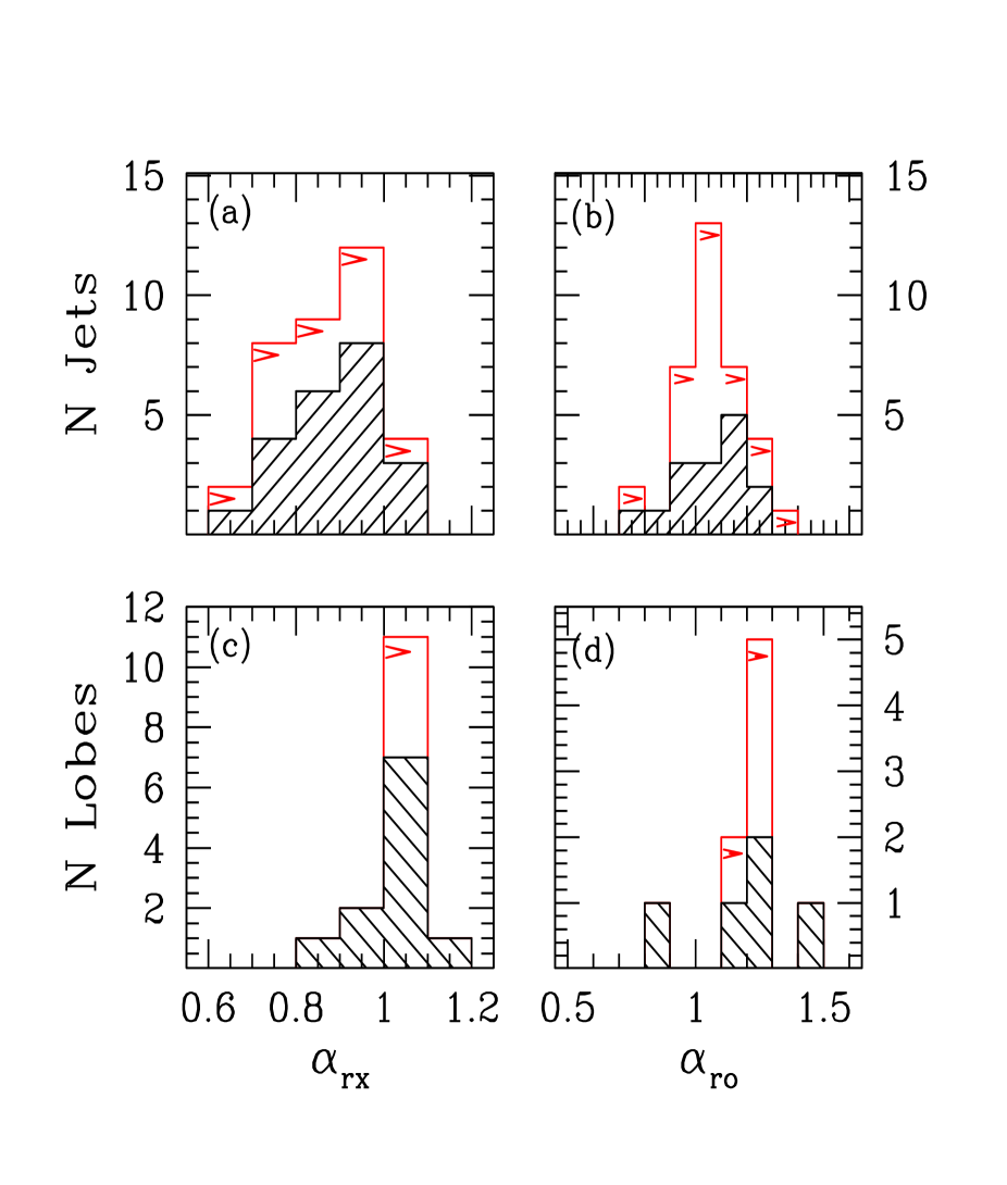
Figure 3: Distributions of the radio-to-X-ray spectral index, $\alpha_{rx}$ (left panels) and for the radio-to-optical index, $\alpha_{ro}$ (right panels). (a) and (b): Distributions of $\alpha_{rx}$ and $\alpha_{ro}$ for the jet knots; (c) and (d): Distributions of $\alpha_{rx}$ and $\alpha_{ro}$ for the lobes. The dashed histograms represent detections, while the arrows represent lower limits.

In Figure 3a we plot the distribution of the radio-to-X-ray spectral index for the jet knots, $\alpha_{rx}$, defined between 5 GHz and 1 keV (see § 4.4 and Tables 5 and 6). The filled histograms represent X-ray detections; upper limits are marked with arrows. As is apparent from the Figure, the $\alpha_{rx}$ distribution is consistent with our selection criteria ($\alpha_{rx}\sim 0.8$). Using the statistical package asurv (Feigelson & Nelson 1985), we estimated the probability $P_{asurv}$ that the observed distribution of $\alpha_{rx}$ in Figure 3a is drawn from a Gaussian distribution centered on $\alpha_{rx}=0.8$, with width equal to the observed width at half maximum in Figure 3a. Depending on the test used within the package, $P_{asurv}$ $\;\buildrel>\over{\sim}\;$90%. The average value of $\alpha_{rx}$ is $\langle\alpha_{rx}\rangle$=0.88 with dispersion $\sigma_{rx}$=0.08.

In Figure 3a, the non-detections span the same range of indices as for the detections. This indicates that, due to non-uniformities in the observations and background, even the flattest bins are not completely covered. Thus, there is reason to expect that essentially all bright radio jets have associated X-ray emission, which would be apparent in deeper and better resolved maps.

Figure 3b shows the distributions of the radio-to-optical index, $\alpha_{ro}$, defined between 5 GHz and 5852 Å (§ 4.4), for the jet knots. As in Figure 3a, the dashed area represents solid optical detections while the arrows indicate the upper limits to the optical flux (Urry et al. 2004). Using asurv, we find a probability $P_{asurv}$ $\;\buildrel<\over{\sim}\;$85% that the observed distribution is consistent with a Gaussian distribution centered on $\alpha_{ro}=0.8$. The average value of $\alpha_{ro}$ in Figure 3b is $\langle\alpha_{ro}\rangle$ = 1.05 with dispersion $\sigma_{ro}$=0.12. We conclude the observed distribution of $\alpha_{ro}$ is consistent with steeper values than assumed. The upper limits are distributed throughout the full range of values for the detections. However, since fewer optical knots were detected, determining the true distribution will require deeper observations.

Although our sample was not optimized for X-ray/optical study of the hotspots/lobes, we detect a fair number of them (Table 4). Specifically, X-ray emission from hotspots/lobes was detected in 7/17 sources, with an optical counterpart in 4 cases. Figures 3c and 3d show the distributions of the $\alpha_{rx}$ and $\alpha_{ro}$ indices for the hotspots/lobes. Both distributions indicate steeper indices than for the jet knots; in fact, the flattest values, easiest to detect, are missing. For Figures 3c and 3d, $\langle\alpha_{rx}\rangle$ = 1.03 and $\sigma_{rx}$=0.05 and $\langle\alpha_{ro}\rangle$ = 1.17 and $\sigma_{rx}$=0.15.

Finally, in 5/17 sources there is a weak X-ray detection of the counterlobe (0723+679, 0838+133, 0836+299, 1040+123, and 1136–135). X-ray emission from the counterlobe of 0838+133 was interpreted by Brunetti et al. (2002) as back-scattered Compton flux, and a similar explanation may hold for 0723+679 (Paper I). While 0723+679, 0838+133, 1040+123, and 1136–135 are powerful FRIIs, the radio galaxy 0836+299 exhibits an FRI morphology and has a radio power similar to an FRI (van Breugel et al. 1986). Both hotspots in the lobe and counterlobe in 0836+299 have an optical counterpart. However, the optical emission from the Northern hotspot is probably due to emission lines (van Breugel et al. 1986). Since our very broad filter does not distinguish emission lines from continuum, we do not quote an optical flux for this feature.

4.2 Jet Multiwavelength Morphologies

X-rays versus radio: Concentrating on a comparison of the radio and X-ray jets in Figure 1, a variety of morphologies is apparent. In most cases, the X-rays track the radio one-to-one, i.e., all X-ray knots have a radio counterpart.

The jet of 1136$-$135 stands out for its remarkable multiwavelength morphology. As clearly shown in Figure 1, there is weak or no radio emission from the inner jet which instead is detected at X-rays (knots $\alpha$, A), and while after knot B at $\sim$ 7^′′ from the core the X-rays start to fade, the radio emission picks up, peaking at $\sim$ 10^′′ from the nucleus. A similar situation occurs for 1510$-$089, where the jet morphology is rather similar at radio and X-rays in the inner parts while the radio-to-X-ray flux density ratio increases dramatically after 8^′′. 3C 273 is another example of this morphology (Sambruna et al. 2001).

In 1040+123, 1741+279, and 2251+134, the X-ray knots are not resolved as they are located at $\;\buildrel<\over{\sim}\;$1^′′ from the strong core, and we can not comment on these jets morphology. Higher-resolution X-ray observations are needed to study these jets.

X-rays versus optical: As discussed above, seven jets have detections at both X-rays and optical, while two have only optical counterparts. For most of the optical/X-ray jets, optical emission is confined within 3–4^′′ from the nucleus, while X-ray emission extends to larger distances. This may be due to the broader $\alpha_{ro}$ distribution where a detection would require a deeper HST observation. Because of the many non-detections we cannot distinguish between a steep $\alpha_{ro}$ (too steep for the short HST exposure) and a true lack of optical emission from the jet. The three exceptions are 1040+123, 1136$-$135, and 1150+497, where the optical jet is as long as (1150+497) or longer then (1040+123, 1136$-$135) the X-ray jet.

Recent Chandra studies showed that X-ray emission from FRI jets may be common (e.g., Worrall et al. 2001). In the only FRI source of our sample, 0836+299, weak X-ray excess counts over the background are detected in the ACIS image in correspondence to the inner radio jet at $\sim$ 2^′′ (Figure 1), well inside the optical galaxy. However, a similar X-ray feature is also present at opposite azimuth, raising the possibility that the X-ray emission from the radio feature is spurious. No optical counterpart is detected in our HST image, after subtracting the host galaxy.

4.3 Continuous Intra-knot X-ray Emission

Interestingly, in a few cases there is continuous, weak intra-knot X-ray emission. A clear example is 0605$-$085, where the inner jet between knots A and B shows smooth X-ray emission, with no apparent compact knots. Other candidates for continuous intra-knot X-ray emission are 0838+133 and 1136$-$135; however, in 1136$-$135 the optical knots are compact. While the limited ACIS resolution may conspire to produce diffuse emission where many small compact knots are instead present (or smearing out the photons from nearby strong knots), in 0605$-$085 the extension of the continuous X-ray emission is at least 2^′′, larger than the S3 FWHM resolution, and so it is significant in this source. A brief discussion of the possible origin of the intraknot X-ray emission in given below (§ 5.1).

Emission from the inner jet was also detected in PKS 0637$-$752 in a 100-ks ACIS-S exposure (Chartas et al. 2000), with a different spectrum than the external part of the jet, and in 3C 273 in the inner 10^′′ (Marshall et al. 2001). In the latter object, the inner radio/X-ray jet was recently detected in the optical band with the ACS camera on HST (Martel et al. 2003).

4.4 Spectral Energy Distributions

The Spectral Energy Distributions (SEDs) of the radiation emitted by the detected features provide basic information on the emission mechanisms. We caution, however, that the derived flux densities refer mainly to unresolved sources, thus the size of the emission region is uncertain, at least at X-rays. In the optical, most of the knots are unresolved even at the HST resolution (0.2^′′; Urry et al. 2004), and we will use an upper limit to the source size in the modeling (see below). For consistency, we extracted flux densities at the three wavelengths from the same spatial region around the knot. Since the X-rays have the lowest resolution, the aperture of the extraction region was fixed at 1^′′ or 1.5^′′. The extraction region was centered on the position of the X-ray knot, or of the optical one when no X-ray feature was detected.

Following Paper I, radio fluxes for those features well separated from the nucleus were extracted from the same aperture as the X-ray flux (see section 3.1). The optical fluxes were extracted as described in § 3.2. The unabsorbed X-ray flux at 1 keV was derived from the fit to the ACIS spectrum of the knot, when available (Table 2a), or using a power law with average X-ray photon index, $\langle\Gamma_{knots}\rangle=1.52$. The optical fluxes are corrected for Galactic extinction. Intrinsic reddening, impossible to estimate with the data in hand, is highly unlikely as the line of sight is close to the jet axis and the resolved knots are at large distances from the nucleus.

The optical flux plays a critical role in the interpretation of the SED. Specifically, if the optical emission lies on the extrapolation between the radio and X-ray fluxes or above it, the SED is compatible with a single electron spectrum extending to high energies; instead, if the optical emission falls well below the extrapolation, it argues for different spectral components (and therefore different mechanisms or two electron populations) below and above the optical range (e.g., synchrotron and IC respectively). Thus, an up-turn of the spectrum in the X-ray band with respect to the radio-optical extrapolation, yielding an optical-to-X-ray index $\alpha_{ox}$ flatter than the radio-to-optical index $\alpha_{ro}$, is a signature of a separate spectral component in the X-ray band. Conversely, when synchrotron dominates we expect $\alpha_{ro}$ $\;\buildrel<\over{\sim}\;$$\alpha_{ox}$, with the inequality holding when radiative losses are important in the X-ray band.

Table 5a-b lists the radio, optical, and X-ray flux densities, or upper limits to them, for the jet knots, while Table 6a-b lists the same for the lobes. Also listed in both Tables are the broad-band indices $\alpha_{ro}$, $\alpha_{ox}$, and $\alpha_{rx}$, defined as the spectral indices between 5 GHz and 5852 Å, 5852 Å and 1 keV, and 5 GHz and 1 keV, respectively.

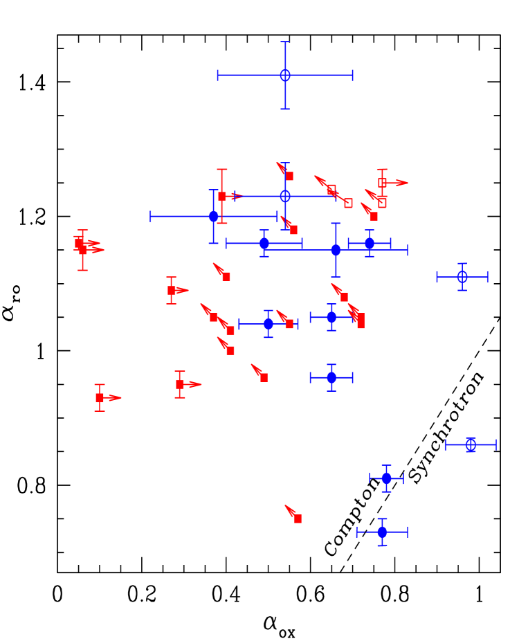
Figure 4: Plot of the radio-to-optical spectral index, $\alpha_{ro}$, versus the optical-to-X-ray index, $\alpha_{ox}$. The filled circles are for the jet knots (Table 5), while the open circles are for the lobes (Table 6). The squares are for non-detections. The dashed line marks the locus where $\alpha_{ox}=\alpha_{ro}$. Knots lying above the dashed line have a concave SED, where the X-rays belong to a different spectral component than the longer wavelengths; IC probably dominates in these sources for the X-ray production. Knots below the dashed line have a convex SED, and the X-rays are interpreted as due to synchrotron emission (see text).

Figure 4 shows the plot of $\alpha_{ro}$ versus $\alpha_{ox}$ for all the jet features for which a firm detection at either optical or X-rays is available. The dotted line, corresponding to $\alpha_{ro}=\alpha_{ox}$, separates the SEDs of the various features between concave (left) and convex (right). In the large majority of the jet knots, X-rays are not an extension of the radio-to-optical synchrotron spectrum; the X-ray flux lies above the extrapolation from the radio-to-optical slope. Similarly, most hotspots have concave SEDs.

Figure 5 shows the relative variation of the X-ray-to-radio flux ratios along the jet. In the Figure, $\alpha_{rx}$ is plotted vs. the projected distance of the knots from the core. The uncertainties on $\alpha_{rx}$ are listed in Table 5. Remarkably, a trend is present in each jet of decreasing X-ray-to-radio flux (increasing $\alpha_{rx}$) from the innermost to the outermost regions of the jet. Note that the trend is present at large distances from the core, where contamination of the X-ray flux from the PSF wings is negligible. A similar but less robust trend of decreasing optical-to-radio flux appears in Figure 6, where $\alpha_{ro}$ is plotted versus the projected distance. We will comment on these trends in § 5.3.

5 Origin of the X-ray emission

5.1 Clues to the X-ray emission mechanism

As seen in Figure 1, the detected jets exhibit a variety of multiwavelength morphologies. In a sense, each jet appears to be unique in its detailed properties and deserves a detailed individual study. In fact, we have already secured deeper follow-up observations in Chandra AO4 and multi-color HST ACS exposures of 1136$-$135 and 1150+497.

General clues to the origin of the X-ray emission can be offered by the study of multiwavelength SEDs for the different emission features along the jet. It is well established that the radio emission is due to the synchrotron mechanism. Thus, the simplest hypothesis to be considered is whether the optical and X-ray emission could be due to synchrotron emission from the same electron distribution (in a simple, zero-order approximation). In that case one would expect the radiated spectrum to follow a power law or to steepen at higher energies due to radiation losses. From the plot of $\alpha_{ro}$ versus $\alpha_{ox}$ (Figure 4) it appears that this may be true for at most two cases which fall close to the line for which $\alpha_{ro}=\alpha_{ox}$. One of them corresponds to knot A in the jet of 1136$-$135, the other to knot A of 1928+738. However, the vast majority of knots lie in the region $\alpha_{ro}>\alpha_{ox}$, showing X-ray emission in excess of the extrapolation from lower energies.

In order to explain the excess X-ray radiation via the synchrotron mechanism, it is necessary to invoke an extra component in the population of relativistic electrons (e.g., Wilson & Yang 2002). A particularly elegant possibility was proposed by Dermer & Atoyan (2002), whereby relativistic electrons are continuously injected and subject to radiative losses dominated by inverse-Compton cooling. However, due to the Klein-Nishina suppression of the Compton cooling rate, high-energy electrons suffer less cooling compared to low-energy ones, naturally developing a high-energy excess in the spectrum. In this hypothesis the observed X-rays would be produced by very-high energy electrons.

Alternatively, in a synchrotron plus inverse Compton (IC) scenario, a single power-law electron population can be responsible for emitting the radio via synchrotron and the X-rays via IC, any external seed photon field being amplified if the jet is still relativistic on the relevant scale. Note that these knots occur predominantly at large distances from the core. As the jets are very long (projected lengths $\sim$ 50–100 kpc, intrinsic lengths possibly 2-3 times longer, perhaps 10 times longer) and extend outside the host galaxy, the most likely source of seed photons for IC is provided by the Cosmic Microwave Background (CMB) photons (Tavecchio et al. 2000), whose energy density scales as $(1+z)^{4}$. For plausible values of the Doppler factor and the magnetic field ($\delta\sim 10$, $B\sim 10\mu$G), the energy of the electrons radiating via synchrotron in the radio and via IC in the X-rays is expected to be relatively close ($\gamma_{r}=1000$, $\gamma_{X}=100$), hence a similar jet morphology at both wavelengths is natural, as observed in most knots. X-rays from these features are therefore likely explained by the IC/CMB model, on both spectral and morphological grounds. However, starlight photons can be important for knots within the galaxy, within a few tens of kpc of the core (estimated in a similar way to Stawarz, Sikora, & Ostrowski 2003). These photons would be upscattered in the X-ray band by very low-energy electrons, $\gamma\sim 2$. Due to the limited ACIS resolution, emission from the innermost knots cannot be easily quantified.

A discriminant between synchrotron and IC origin for the X-ray emission is the particle radiative lifetime. One would expect shorter radiative lifetimes, and thus more compact emission regions, at the shorter wavelengths in the synchrotron model, whereby X-rays derive from high-energy electrons. The morphology of the 1136–135 jet suggests synchrotron is important in at least some knots. This is supported by the radio-to-X-ray spectral energy distribution of knot A in 1136$-$135, which indeed does not show an X-ray excess and was fitted by synchrotron emission in Paper I.

A direct consequence of the IC/CMB model is that X-rays are produced by low-energy electrons, characterized by an extremely large cooling timescale. Since the electrons can not cool within the short distance of a knot, we expect continuous X-ray emission due to their streaming along the jet. Indeed, in a few cases intraknot emission is visible in our Chandra images (§ 4.3). Therefore, it is possible to accommodate the knotty morphology with the virtually infinite cooling time of X-ray electrons, assuming that knots just represent local enhancement of the surface brightness, as expected in a shock compression scenario. Due to the limited sensitivity of our data, we can not draw firm conclusion. As discussed in Tavecchio, Ghisellini, & Celotti (2003), the presence of isolated knots would represent a severe problem for the simplest version of the IC/CMB model. A possible way out would be to postulate that the low-energy electrons are cooled through adiabatic losses, effective only if the source can expand enough to cool electrons from $\gamma\sim 100$ to $\gamma\sim 10$. These considerations lead Tavecchio et al. (2003) to propose that the emission from a “knot” is instead due to a large number of unresolved expanding “clumps”. Deeper observations at higher resolution are needed to further investigate possible knot substructures.

5.2 Reproducing the SEDs

To investigate quantitatively the jet physical properties within the simple homogeneous synchrotron + IC/CMB model, we modeled the SEDs of the knots which were detected at both optical and X-rays. Clearly, with only three measured fluxes the models are underconstrained. However, in the cases where X-rays can be attributed to IC/CMB the model parameters can be fixed if the equipartition assumption is adopted.

A significant uncertainty of present observations concerns the size of the emitting region(s). In what follows, we assume that the emitting region is consistent at the three wavelengths examined and adopt a region size of 1^′′ radius, corresponding to the X-ray resolution and the area from which fluxes were extracted.

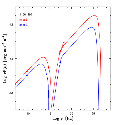
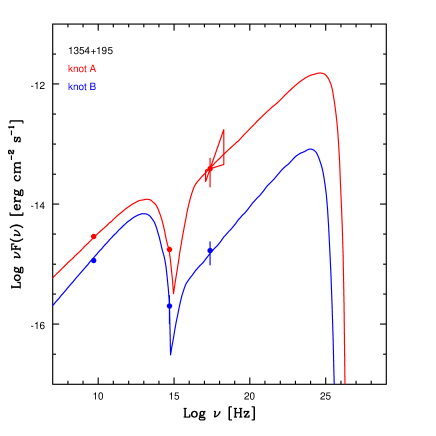
Figure 7: Selected radio-to-X-ray Spectral Energy Distributions (SEDs) and best-fit models assuming a synchrotron + IC/CMB model, with the parameters reported in Table 7.

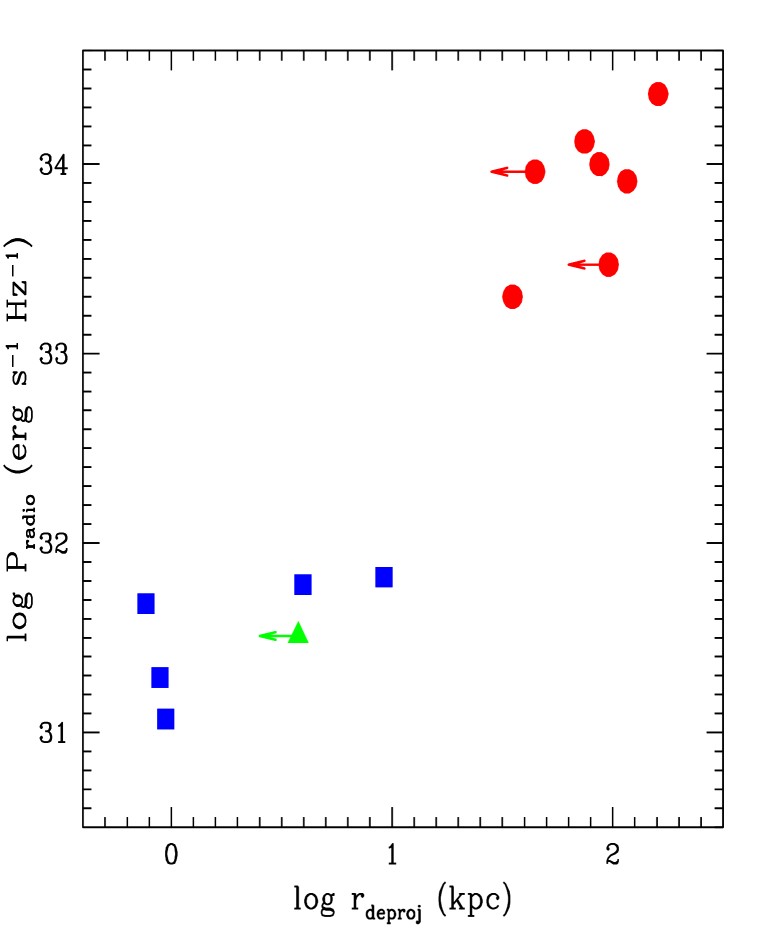
Figure 8: Plot of the total radio power versus the deprojected distance of the first detected optical/X-ray knot. The circles are the FRIIs of our sample, while the squares are FRI sources from the literature for which sufficient information is available (see text). The triangle is the only FRI of our sample, 0836+299. In more powerful sources, the first detected knot is at larger distances from the core than in lower-power sources.

We refer to Tavecchio et al. (2000) and Paper I for a full description of the model. Briefly, the emitting region is assumed to be spherical with radius $R$ and in motion with a bulk Lorentz factor $\Gamma$ at an angle $\theta$ with respect to the line of sight. Since fluxes are extracted within a circle of radius 1^′′, we fix the dimension $R$ (in cm) corresponding to this angular size. Note that this is different than Paper I, where for simplicity we considered a unique value of radius for all the sources. The emitting region is homogeneously filled by high-energy electrons, with a power-law energy distribution $N(\gamma)=K\gamma^{-n}$ extending from $\gamma_{\rm min}$ to $\gamma_{\rm max}$. Electrons emit radiation through synchrotron and IC/CMB mechanisms. The low-energy limit of the electron distribution $\gamma_{\rm min}$ is well constrained by the condition that the low-energy part of the IC/CMB component cannot overproduce the observed optical flux. Note that the optical emission in many cases could be attributed either to the high-energy tail of the synchrotron component (in this case the optical spectrum is expected to be soft) or to the low-energy tail of the IC/CMB component (hard optical spectrum expected). The X-ray spectra of the knots in Table 2a are relatively flat in all the cases where the SEDs are consistent with IC/CMB, as expected (e.g., Fig. 8 in Paper I). The parameters of the best-fit models are reported in Table 7. Figure 7 shows representative SEDs for two sources where at least two knots were detected at X-rays and optical in the same jet, with the best-fit models superposed.

For two cases, namely knots A in 1136$-$135 and 1928+738, the optical-radio-X-ray fluxes are consistent with one component, indicating the X-rays are produced via synchrotron. Therefore, in these cases we have reproduced the observed fluxes imposing that the IC/CMB component does not substantially contribute to the X-ray flux: This provides a lower limit on the Doppler factor, that translates into a limit on the bulk Lorentz factor and on the observing angle reported in Table 7. The kinetic and radiative powers derived with the parameters reported in Table 7 confirm the evidence (see also Paper I) that only a small fraction ($\;\buildrel<\over{\sim}\;$0.1%) of the jet kinetic power is dissipated into radiation.

Since our choice of the size of the emitting region based on the Chandra resolution is rather restrictive, we checked the sensitivity of the derived parameters on the assumed volume. Since we know from the optical images that the (optical) knots are unresolved down to $\sim 0.2$^′′, we performed a series of fits assuming a cylindrical region with height 2^′′ (along the jet direction) and radius 0.2^′′. The results of this new set of fits show that the derived parameters are not strongly affected by this change in volume: in particular $\delta$ is slighly larger (about a factor 1.5) and similarly the magnetic field and the electron density change within a factor of 3–4.

5.3 Trends of the emission along the jet

If emission from single knots seems to be well reproduced by the IC/CMB model, further interesting clues to the origin of the high-energy emission and to the global dynamics of the jet originate from examination the overall trends of the SEDs for different knots along the same jet. These were presented in Figures 5 and 6, which show the plots of $\alpha_{rx}$ and $\alpha_{ro}$ versus the projected distance of the knots from the cores. As discussed in § 4.4, the X-ray-to-radio and optical-to-radio flux ratio decreases along the jets.

The trends in the two plots suggest that a common evolution of the conditions along the jet determines the observed properties of the emission features. In a pure “synchrotron+IC/CMB” model, the relative strength of the X-ray and radio emission, which to first order is given by the ratio of the CMB and magnetic densities, is expected to increase, since the magnetic field within the jet presumably decreases and the energy density of the CMB is constant. The observed opposite behaviors could have different origins:

• It could be due to the synchrotron mechanism extending to the X-ray band in the inner knots (due to a higher value of the magnetic field and/or the particle energies), thus providing an additional X-ray component which progressively disappears in the more external knots. This scenario is supported by the case of 1136–135, where a synchrotron emitting inner knot is resolved with ACIS. This interpretation is also supported by the case of 3C 273, where the X-ray emission from the first knot is possibly synchrotron (Marshall et al. 2001). The preliminary analysis of our deeper Chandra and multicolor HST exposures of 1150+497 and 1136–135 also confirm this interpretation.

• An additional component of IC emission could be provided in the innermost knots by the interstellar light photons whose energy density within the galaxy can prevail over the CMB density (e.g. Stawarz et al. 2003). Along the jet this contribution will decrease, producing the observed trend of the X-ray-to-radio flux ratio.

• In a pure IC/CMB scenario, the trend could be attributed to decelerating plasma: the decreasing value of $\Gamma$ translates into a less amplified CMB radiation and thus a lower X-ray flux compared to the radio flux. Elements supporting this view are provided by our modeling of the jet of 1354+195, for which two distinct knots were analyzed (see Table 7). The data require that the bulk Lorentz factor between the two features decrease by a factor of 2, from $\Gamma=14$ (knot A) to $\Gamma=6$ (knot B). At the same time the magnetic field strength and the number of particles increase. (However, remember that we are assuming equipartition, so the magnetic energy density and the electron energy density are linked.)

The trend observed in the $\alpha_{ro}$ profiles can simply be related to the decreasing value of the maximum Lorentz factor of the emitting electrons. This will produce a shift of the synchrotron cutoff toward lower frequencies along the jet and therefore a decreasing optical flux along the jet (note that the same beavior can be mimicked by a decrease of the magnetic field). A better understanding of these and other systematic trends requires more sophisticated theoretical studies than is possible to include here.

5.4 Caveats

It is worth remarking a few caveats affecting our analysis. First, the limited signal-to-noise ratio at both X-ray and optical wavelengths leaves room for alternative interpretations of the SEDs. Second, as already mentioned above, a variety of physical conditions may exist within the relatively large extraction regions we used (1^′′, dictated by the Chandra resolution), for example the emitting particle distributions could be stratified or multiple shocks may exist. While higher angular resolution at X-rays awaits future generations of space-based telescopes, deeper follow-up X-ray and optical observations of the new jets of this survey with Chandra and HST can at least remedy the first limitation of our analysis, in providing accurate X-ray and optical continuum spectra for individual knots, a key test for the emission models.

High-quality X-ray and optical spectra of single knots will be essential to discriminate among the various models, as well as more detailed maps to measure and quantify the positional offsets of the radio, optical, and X-ray peaks. Optical observations are necessary to identify the mechanism responsible for the X-ray emission, as the optical band lies at the intersection of the synchrotron and IC components. We have already taken steps to acquire follow-up observations of selected jets during the Cycle 4 Chandra-HST cycle. Finally, an additional important constraint will be provided by future IR observations with SIRTF, probing a poorly known region in the SEDs where the synchrotron peak (related to the break energy of the synchrotron electron population) is located. Of particular interest will be SIRTF observations of the jets not detected at optical wavelengths, to determine whether this can be due to a lower cutoff energy of the electron distribution.

5.5 Comparison with FRI Jets

Chandra has detected X-ray emission in a handful of low-power FRI sources (Worrall et al. 2001, Hardcastle et al. 2002, 2001). It is interesting to compare their properties to the FRII jets of our sample.

In most FRI jets, the X-ray flux of the detected knots lies on the extrapolation of the radio-to-optical emission. The favored interpretation is that the X-rays are due to synchrotron emission from the same population of electrons responsible for the radio and optical fluxes. The X-ray spectrum of the knot, when available, is also consistent with the low-energy emission, confirming this interpretation. The radio/X-ray morphology of the jet is remarkably similar in all FRIs. In all cases, the X-ray profile of the first detected knot peaks before the radio, yielding a larger X-ray-to-radio flux ratio, or flatter $\alpha_{rx}$, than in the knots further away along the jet. A similar situation occurs for sources close to the FRI/II transition (e.g., 3C 371, Pesce et al. 2001; PKS 0521–365, Birkinshaw et al. 2002).

Thus, the X-ray emission from kpc-scale jets in FRIs and FRIIs appears to be due to different processes, with synchrotron dominating in low-power sources and IC/CMB in high-power sources. However, a closer look to our targets reveals that the FRI/II division of jet emitting mechanisms may not be sharp. Indeed, as discussed above, the inner parts of the powerful FRII jets may be dominated by different production mechanisms for the X-rays, suggesting a change of conditions along the jet. A clear example from our survey is 1136$-$135. In this case, X-rays from the innermost knot A ($\sim$ 5^′′, or 25 kpc) are due to synchrotron emission of high-energy electrons in the jet, while X-rays from external knot B are consistent with IC/CMB (Table 7). Strong particle acceleration is necessary to explain synchrotron X-rays in the inner parts of the jet.

A possibility to account for the FRI/II dichotomy on large-scales is proposed in our companion paper (Tavecchio et al. 2004). We suggest that the main difference between FRI and FRII jets is the location at which the jet pressure becomes comparable to the ambient gas pressure and the jet starts to slow down significantly, giving rise to shocks. Assuming that both FRI and FRII host galaxies have similar gas halos (e.g., Gambill et al. 2003), the discriminating parameter becomes the jet pressure which is related to the jet power (Maraschi & Tavecchio 2003): the more luminous sources (FRIIs) are slowed down later than less luminous ones. If this is true, one expects to observe the sites where dissipation is taking place - the innermost knots - closer to the core in lower-luminosity sources than in the more powerful ones.

To illustrate this point, we plot in Figure 8 the total radio power of the sources versus the deprojected distance of the first detected knot (optical or X-ray). The total radio powers were derived from Cheung et al. (2004), Liu & Xie (1992), and Liu & Zhang (2002). Only the sources for which an estimate of the angle from modeling is available (Table 7) were used. In addition, we plot the same quantities for a few low-power radio galaxies from the literature for which enough information is available (3C 371, Pesce et al. 2001; M87, Wilson & Yang 2002; 3C 31, 3C 66B, Hardcastle et al. 2002, 2001; and NGC 315, Worrall et al. 2003). The only FRI of our sample, 0836+299, is also plotted (triangle). As apparent from Figure 8, low- and high-power sources occupy distinct regions, with the FRIIs having the first detected knots at larger distances from the nucleus than lower-luminosity sources. A trend is also present within the FRII class itself.

We note, however, that the FRIIs in the Figure are at larger redshifts than FRIs. The loss in resolution thus could be introducing a bias, i.e., we are not resolving the innermost knots in the most distant FRIIs. In fact, in 3C 273 ($z$=0.158) optical knots very close (2.7^′′, or projected distance of 7 kpc) to the nucleus were recently detected with the ACS camera on HST (Martel et al. 2003). Clearly, high-resolution sensitive observations of the inner jets in FRIIs are needed to confirm the suggestion of Figure 8. Moreover, the deprojected jet length clearly depends on the assumed (hence model-dependent) value of the viewing angle. In this respect, the choice of the IC/CMB model for the high-power datapoints in Figure 8 could introduce a bias toward small angles and therefore large deprojected lengths. However, other (almost model-independent) indicators such as the core dominance parameter $R_{i}$ and the jet-to-counter jet ratio $J$ (Table 1), suggest small observing angles. Based on these considerations, we are confident that the large deprojected lengths in Figure 8, albeit affected by inevitable uncertainties, are reliable.

Although the scenario depicted above can explain some of the basic differences between FRIs and FRII, the study of the nearest FRI, M87, shows that the situation may be more complex. In this object the X-ray flux belongs to a separate component than the longer wavelength flux. The steep X-ray spectrum suggests synchrotron emission from a separate population of particles (Wilson & Yang 2002), indicating jet inhomogeneities. Moreover, we recall that there are also indications that the jet can have a velocity structure, with a fast spine surrounded by a slower moving layer (as originally proposed by Laing et al. 1993). Synchrotron emission would be produced in the walls of the jet, while IC/CMB would predominate in the beamed emission concentrated in the spine.

6 Summary and Conclusions

We presented short Chandra and HST observations of a sample of 17 radio jets. One goal of the survey was to establish in a systematic way the relation between X-ray/optical and radio emission from extragalactic jets. The survey was therefore designed to provide at least a detection in X-rays for a radio-to-X-ray spectral index $\alpha_{rx}=0.8$, and in the optical for $\alpha_{ro}=0.8$. The short exposures were designed to search for the X-ray and optical counterparts of the radio jets, and start addressing their physical properties through multiwavelength imaging.

We detect X-ray emitting knots in 10/17 (59%) jets, with a similar detection rate for the optical features. This is actually a lower limit to the number of X-ray emitting knots, as several radio- and optically-detected features are too close to the core ($\;\buildrel<\over{\sim}\;$1–2^′′) to be clearly resolved with ACIS. Moreover, as discussed above, the non-detections are most likely related to incompleteness rather than $\alpha_{rx}$ indices steeper than expected (Figures 3a). We can thus conclude that X-ray emission from extended radio jets with $\alpha_{rx}\sim 0.8$ is common in AGN, and it is consistent with being a characteristic of essentially all bright radio jets.

The rate of detection in Table 2a is similar for FSRQs and SSRQs, $\sim$ 60%. The presence of a large number of FSRQs in the sample (Table 1) is a direct indication that our sample is biased towards beamed objects. Thus, the detection rates for jets refer to lines of sight close to the jet axis at both X-rays and optical. This is in agreement with previous optical studies (Parma et al. 2003, Sparks et al. 1995), which concluded that jet optical emission is preferentially detected in those sources with larger beaming, i.e., where the jet is closer to the line of sight. In fact, the two jets in our sample with the lowest values of the core-to-total radio power, 0802+103 ($R_{i}\sim 0.03$) and 0836+299 ($R_{i}\sim 0.06$), are not detected at either optical or X-rays.

In our sample, there is no obvious dependence of the detection rates on redshift. The most distant jet (0802+103 at $z$=1.96) is not detected at X-rays or optical, however, this source has a lesser defined radio jet (Figure 1) and is the most lobe-dominated source in the sample. The second most distant, 1040+123 at $z$=1.03, is well-detected at optical wavelengths but only upper limits are present at X-rays. The third most distant, 1055+018 at $z$=0.88, is not detected. A larger, systematic sample of high-redshift sources with well-defined radio data is needed to confirm the suggestion (Schwartz 2002) that X-ray emission is common at cosmological redshifts as a result of an increased CMB density.

In summary, the main results of our paper are:

• X-ray and optical emission is detected in $\sim$ 60% of the jets, with $\langle\alpha_{ro}\rangle\sim 1.0$ and $\langle\alpha_{rx}\rangle\sim 0.8$.

• The non-detections in the X-rays are due to incompleteness rather than $\alpha_{rx}$ indices steeper than expected, meaning essentially all radio jets have X-ray emission at some intensity level. The observed distribution of $\alpha_{ro}$ indices is consistent with steeper values than assumed.

• In most knots the X-ray flux lies above the extrapolation of the radio-to-optical continuum, indicating a separate spectral component.

• Interpreting the X-ray emission of these knots as due to inverse Compton scattering off the CMB photons, yields relativistic jets on kpc scales, with plasma Lorentz factors $\Gamma_{jet}\sim 3-15$, and very low ($<$ 0.1%) radiative efficiencies.

• In a few knots the X-ray flux lies below or on the extrapolation of the radio-to-optical continuum. Here the X-rays are likely to be due to synchrotron emission from the same population of relativistic particles responsible for the longer wavelengths.

• Spectral changes along the jets are observed, with the X-ray-to-radio and optical-to-radio flux ratios decreasing from the inner to the outer regions.

• The trend of decreasing X-ray-to-radio flux ratios can be either the results of 1) an additional X-ray producing process in the inner jet (synchrotron or inverse Compton scattering of starlight), or 2) in the IC/CMB scenario, decelerating plasma. The trend in $\alpha_{ro}$ could simply be due to a decrease of the electrons Lorentz factor along the jet.

Several questions remain open. Most fundamental one is the origin of the bright X-ray emission from kpc-scale jets. As discussed above, the IC/CMB process appears to account satisfactorily for the flat optical-to-X-ray spectral indices of most knots, at least in the external part of the jets, but implies the presence of relativistic bulk motion at large distances from the core. This is in contrast with radio studies showing only modest bulk velocities at such distances (e.g., Wardle & Aaron 1997), but is consistent with jet one-sidedness and with depolarization asymmetries (Garrington et al. 1988). Additional contributions to the X-ray emission may be present along the jet, e.g., IC of the host galaxy starlight, which could account for the decreasing X-ray-to-radio flux ratios along the jet (see above). Possible inhomogeneities in the jet (multiple shocks or particle distributions) in space or/and time are additional complicating factors.

In some FRII jets we observe “mixed” emission with synchrotron dominating in the inner parts of the jet (e.g., 1136–135, 3C 273). The rate of occurrence of this is still unclear, as is its physical origin.

Finally, we note that the X-ray spectral indices measured in the large majority of the jets knots are flat, $\alpha_{X}\sim 0.5$, indicating that most of the jet luminosity is emitted at $\gamma$-rays. This raises the interesting possibility of future GLAST detections. Given that radio jets might be bright at large redshifts (Schwartz 2002), it would not be surprising if extended jets would be found to be significant contributors to the $\gamma$-ray background. While GLAST lacks sufficient angular resolution to separate the kpc-scale jet from the bright core, variability studies could conceivably be used to discriminate the origin of the gamma-ray emission.

Figure 1: Chandra ACIS-S images of the radio jets of our sample in the 0.5–8 keV energy range. Overlaid are the radio contours from archival VLA data. Both the colors and the contours are plotted logarithmically, in steps of factor 2. The Chandra image is smoothed with a Gaussian of width $\sigma$=0.3^′′, yielding a resolution of 0.86^′′ FWHM. The radio image was restored with a circular beam (see Appendix). North is up and East to the left.

Figure 2: Chandra ACIS-S images in the 0.5–8 keV energy range of selected jets of our sample, showing the innermost jet regions close to the core. North is up and East to the left.

Figure 5: Plot of the radio-to-X-ray spectral index for the knots of individual jets (in different symbols) versus the projected distance of the knot from the core. The circles mark the innermost knots where contamination from the PSF wings could be present. The uncertainties on $\alpha_{rx}$ are listed in Table 5 and 6. Interestingly, the X-ray-to-radio flux ratio decreases with increasing distance along the jet.

Figure 6: Same as for Figure 5, but for the radio-to-optical index. Again, the optical-to-radio flux ratio decreases with increasing distance along the jet.

References

- (1)
- (2) Akujor, C.E. & Garrington, S.T. 1991, MNRAS, 250, 644
- (3)
- (4) Aldcroft, T.L., Elvis, M., & Bechtold, J. 1993, AJ, 105, 2054
- (5)
- (6) Birkinshaw, M., Worrall, D. M., & Hardcastle, M. J. 2002, MNRAS, 335, 142
- (7)
- (8) Bridle, A. H., Hough, D. H., Lonsdale, C. J., Burns, J. O., & Laing, R.A. 1994a, AJ, 108, 766
- (9)
- (10) Bridle, A. H. & Greisen, E. W. 1994b, AIPS Memo 87 (NRAO: Charlottesville)
- (11)
- (12) Bridle, A.H. & Perley, R.A. 1984, ARA&A, 22, 319
- (13)
- (14) Brunetti, G., Bondi, M., Comastri, A., & Setti, G. 2002, A&A, 381, 795
- (15)
- (16) Celotti, A., Ghisellini, G., & Chiaberge, M. 2001, MNRAS, 321, L1
- (17)
- (18) Chartas, G. et al. 2002, ApJ, 565, 96
- (19)
- (20) Chartas, G. et al. 2000, ApJ, 542, 655
- (21)
- (22) Cheung, C.C. et al. 2004, in prep.
- (23)
- (24) Cheung, C.C. 2002, ApJ, 581, L15
- (25)
- (26) Dermer, C. & Atoyan, A. 2002, ApJ, 568, L81
- (27)
- (28) Fanaroff, B.L. & Riley, J.M. 1974, MNRAS, 167, 31P
- (29)
- (30) Feigelson, E.D., Schreier, E.J., Delvaille, J.P., Giacconi, R., Grindlay, J.E., & Lightman, A.P. 1981, ApJ, 251, 31
- (31)
- (32) Feigelson, E.D. & Nelson, P.I. 1985, ApJ, 293, 192
- (33)
- (34) Gambill, J.K., Sambruna, R.M., et al. 2003, A&A, 401, 505
- (35)
- (36) Garrington, S.T., Leahy, J.P., Conway, R.G., & Laing, R.A. 1988, Nature, 331, 147
- (37)
- (38) Gehrels, N. 1986, ApJ, 303, 336
- (39)
- (40) Hardcastle, M.J., Birkinshaw, M., Cameron, R.A., Harris, D.E., Looney, L.W., & Worrall, D.M. 2002a, ApJ, 581, 948
- (41)
- (42) Hardcastle, M.J., Worrall, D.M., Birkinshaw, M., Laing, R.A., & Bridle, A.H. & 2002b, MNRAS, 334, 182
- (43)
- (44) Hardcastle, M.J., Birkinshaw, M., & Worrall, D.M. 2001, MNRAS, 326, 1499
- (45)
- (46) Hummel, C. A. et al. 1992, A&A, 257, 489
- (47)
- (48) Kronberg, P.P., Zukowski, E.L.H., & Perry, J.J. 1990, ApJ, 355, L31
- (49)
- (50) Laing R. A., 1993, in Burgarella D., Livio M., O’Dea C.P., eds Space Telescope Sci. Inst. Symp. 6: Astrophysical Jets. Cambridge University press, Cambridge, p. 95
- (51)
- (52) Liu, F.K. & Xie, G.Z. 1992, A&AS, 95, 249
- (53)
- (54) Liu, F. K. & Zhang, Y. H. 2002, A&A, 381, 757
- (55)
- (56) Mack, K.-H., Kerp, J., & Klein, U. 1997, A&A, 324, 870
- (57)
- (58) Maraschi, L. & Tavecchio, F. 2003, ApJ, 593, 667
- (59)
- (60) Marshall, H.L. et al. 2001, ApJ, 549, L167
- (61)
- (62) Martel, A.R. et al. 2003, AJ, 125, 2964
- (63)
- (64) Morrison, R. & McCammon, D. 1983, ApJ, 270, 119
- (65)
- (66) O’Dea, C.P., Barvainis, R., & Challis, P.M. 1988, AJ, 96, 435
- (67)
- (68) Orr, M. J. L. & Browne, I. W. A. 1982, MNRAS, 200, 1067
- (69)
- (70) Owen, F.N. & Puschell, J.J. 1984, AJ, 89, 932
- (71)
- (72) Parma, P. et al. 2003, A&A, 397, 127
- (73)
- (74) Pesce, J.E. et al. 2001, ApJ, 556, L79
- (75)
- (76) Price, R., Gower, A.C., Hutchings, J.B., Talon, S., Duncan, D., & Ross, G. 1993, ApJS, 86, 365
- (77)
- (78) Rusk, R. 1988, Ph.D. Thesis, University of Toronto
- (79)
- (80) Saikia, D.J., Shastri, P., Cornwell, T.J., Junor, W., & Muxlow, T.W.B. 1989, Journal of Astrophysics and Astronomy, 10, 203
- (81)
- (82) Sambruna, R.M. et al. 2002, ApJ, 571, 206 (Paper I)
- (83)
- (84) Sambruna, R.M. et al. 2001, ApJ, 549, L161
- (85)
- (86) Shepherd, M.C., Pearson, T.J., & Taylor, G.B. 1994, BAAS, 26, 987
- (87)
- (88) Scarpa, R. & Urry, C.M. 2002, New AR, 46, 405
- (89)
- (90) Schwartz, D.A. 2002, ApJ, 569, L23
- (91)
- (92) Schwartz, D.A. et al. 2000, ApJ, 540, L69
- (93)
- (94) Sparks, W.B. et al. 1995, ApJ, 450, L55
- (95)
- (96) Sparks, W.B., Biretta, J.A., & Macchetto, F. 1994, ApJS, 90, 909
- (97)
- (98) Stawarz, L., Sikora, M., & Ostrowski, M. 2003, ApJ, in press (astro-ph/0306251)
- (99)
- (100) Tavecchio, F., Maraschi, L., Sambruna, R.M., Urry, C.M., Cheung, C.C., Gambill, J.K., & Scarpa, R. 2004, ApJ, submitted
- (101)
- (102) Tavecchio, F., Ghisellini, G., & Celotti, A. 2003, A&A, 403, 83
- (103)
- (104) Tavecchio, F., Maraschi, L., Sambruna, R.M., & Urry, C.M. 2000, ApJ, 544, L23
- (105)
- (106) Thompson, A. R., Clark, B. G., Wade, C. M., & Napier, P. J. 1980, ApJS, 44, 151
- (107)
- (108) Urry, C.M. et al. 2004, ApJ, in prep.
- (109)
- (110) van Breugel, W.J.M., Heckman, T.M., Miley, G.K., & Filippenko, A.V. 1986, ApJ, 311, 58
- (111)
- (112) Wardle, J.F.C. & Aaron, S.E. 1997, MNRAS, 286, 425
- (113)
- (114) Wilson, A.S. & Yang, Y. 2002, ApJ, 568, 133
- (115)
- (116) Wilson, A.S., Young, A.J., & Shopbell, P.L. 2001, ApJ, 547, 740
- (117)
- (118) Worrall, D. M., Birkinshaw, M., & Hardcastle, M. J. 2003, MNRAS, 343, L73
- (119)
- (120) Worrall, D. M., Birkinshaw, M., & Hardcastle, M. J. 2001, MNRAS, 326, L7
- (121)