The Zeeman effect in the G band

Abstract

We investigate the possibility of measuring magnetic field strength in G-band bright points through the analysis of Zeeman polarization in molecular CH lines. To this end we solve the equations of polarized radiative transfer in the G band through a standard plane-parallel model of the solar atmosphere with an imposed magnetic field, and through a more realistic snapshot from a simulation of solar magneto-convection. This region of the spectrum is crowded with many atomic and molecular lines. Nevertheless, we find several instances of isolated groups of CH lines that are predicted to produce a measurable Stokes V signal in the presence of magnetic fields. In part this is possible because the effective Landé factors of lines in the stronger main branch of the CH A${}^{2}\Delta$–X${}^{2}\Pi$ transition tend to zero rather quickly for increasing total angular momentum $J$, resulting in a Stokes $V$ spectrum of the G band that is less crowded than the corresponding Stokes $I$ spectrum. We indicate that, by contrast, the effective Landé factors of the $R$ and $P$ satellite sub-branches of this transition tend to $\pm 1$ for increasing $J$. However, these lines are in general considerably weaker, and do not contribute significantly to the polarization signal. In one wavelength location near 430.4 nm the overlap of several magnetically sensitive and non-sensitive CH lines is predicted to result in a single-lobed Stokes $V$ profile, raising the possibility of high spatial-resolution narrow-band polarimetric imaging. In the magneto-convection snapshot we find circular polarization signals of the order of 1% prompting us to conclude that measuring magnetic field strength in small-scale elements through the Zeeman effect in CH lines is a realistic prospect.

1 Introduction

Apart from convective phenomena like the granulation most features we observe in the solar atmosphere are due to the presence of magnetic fields. The dynamics of this magnetic field lie at the root of solar activity, giving rise to variable amounts of UV, X-ray and particle radiation that influence not only Earth climate, but also our daily lives in a society that depends more and more on technology. Thus, there is a real incentive to understand, and eventually be able to predict, the behavior of the solar magnetic field. While larger scale magnetic field concentrations like sunspot are more evident, longer lived, and easier to observe, the field on the solar surface seems to be distributed predominantly in small-scale magnetic elements like micropores, network bright points and low contrast internetwork fields (Stenflo, 1994).

Because of their small size, characteristically $0^{\prime\prime}\!\!.25$ (Muller, 1985; Berger et al., 1995; Berger & Title, 2001), at or below the resolution limit of current solar instrumentation, and their rapid time scale of evolution of 10-100 sec, near sustainable cadence of multi-wavelength observations, the morphology, thermal structure and dynamics of small-scale flux concentrations is difficult to study. Despite a characteristic field strength in the kilo Gauss range (Stenflo, 1973), the small sizes of magnetic elements result in low values of the magnetic flux and make the field difficult to observe. Therefore, long integration times are needed to reach the required magnetograph sensitivity if the elements remain unresolved, and this results in smeared images due to the short dynamical time scales of the elements. Fortunately, indirect methods which allow much shorter exposure times exist to examine the structure of magnetic elements, and to follow their evolution. In particular, these methods involve imaging the Sun in wideband (of order 1 nm) filters centered on molecular band heads towards the blue end of the spectrum. Examples are the band head at 388.3 nm due to B${}^{2}\Sigma$–X${}^{2}\Sigma$ electronic transitions of CN (Sheeley, 1971), and the so-called G band (originally designated by Fraunhofer, 1817) around 430.5 nm due to A${}^{2}\Delta$–X${}^{2}\Pi$ transitions of the CH molecule (Muller et al., 1989; Muller & Roudier, 1992; Muller et al., 1994; Berger et al., 1995; van Ballegooijen et al., 1998; Berger & Title, 2001).

In these molecular wideband images the magnetic elements appear as subarcsecond sized bright points with contrasts of typically 30%, compared to the average photosphere (Berger et al., 1995). Berger & Title (2001) find that G-band bright points are cospatial and comorphous with magnetic elements in intergranular lanes to within $0.^{\prime\prime}\!\!24$. Also in strong photospheric lines (Chapman & Sheeley, 1968; Spruit & Zwaan, 1981) and the wings of chromospheric lines like H$\alpha$ (Dunn & Zirker, 1973), and Ca II K (Mehltretter, 1974) bright points seem to coincide with magnetic field concentrations. However, the cores of these lines are considerably darker than the integrated G-band intensity and require much narrower bandpasses, making imaging in them much less practical. Until now measurement of magnetic field strength in molecular bright points has had to rely on cospatial magnetograms in magnetically sensitive atomic lines. This is an arduous process, which involves careful alignment of images taken at different wavelengths and a relative “destretching” of images taken at different times to prevent contamination of the magnetogram signal due to seeing induced image distortions. In addition, not every magnetic element has an associated bright point or vice versa, at a given time, although both Muller et al. (2000) and Berger & Title (2001) conclude that there is a one-to-one correspondence when the temporal evolution of the magnetic field and bright grains is followed.

An important point in the diagnostic use of bright point imaging for the study of magnetic element dynamics and morphology is the question of why the associated bright points are particularly bright in the molecular band heads. Model calculations of G-band brightness in semi-empirical fluxtube atmospheres provide reasonable values for the bright point contrast (Sánchez Almeida et al., 2001; Rutten et al., 2001; Steiner et al., 2001). Flux-tube models are hotter than the quiet Sun in the layers producing the observed light. They are evacuated owing to the presence of a magnetic field, thus allowing us to observe deep and therefore hot photospheric layers. For this very reason, Sánchez Almeida et al. (2001) concluded that G-band contrast in the bright points is enhanced compared to the surrounding photosphere because the opacity in the CH lines is less affected by the higher temperatures present in magnetic elements than the continuum opacity, which is mostly due to H^-. In the continuum a rise in temperature leads to a higher formation height of intensity at consequently lower temperatures. On the other hand, in the G band the formation height remains more or less constant (because of the increase in H^- opacity and decrease in CH line opacity through dissociation) so that the emergent intensity reflects the higher temperatures. Similarly, Rutten et al. (2001) emphasized that the evacuation of magnetic elements due to the requirement of pressure balance with the non-magnetic surroundings leads to excess CH dissociation making the G band relatively more transparent, thereby exposing hotter layers below. This has been clearly illustrated by Uitenbroek (2003) by modeling the G-band intensity in a snapshot from a three-dimensional simulation of solar magneto-convection. That the CH concentration is strongly reduced in evacuated flux-tube regions is logical because the molecular concentration depends quadratically on density if the molecular dissociation is not controlled by radiation, which seems to be indeed the case as pointed out by Sánchez Almeida et al. (2001). Such a quadratic dependence on density would explain why CH lines show stronger weakening than atomic lines in the G band (Langhans et al., 2001), and cause higher bright-point contrast in the CH and CN band heads than in atomic line cores, because in the solar photosphere atomic ionization is mostly dominated by the radiation field, making the opacity in atomic lines only linearly dependent on the density in the flux concentrations.

In this paper we propose a technique that hopefully will allow us to shed further light on the relationship between the magnetic field in the bright points and their increased contrast, namely the measurement of the field through analysis of the polarization signal due to the Zeeman effect in the CH lines that make up the bulk of the opacity in the G band. Over the last few years, we have witnessed an increasing interest in using molecular line polarization as a tool for magnetic field diagnostics, concerning both the molecular Zeeman effect (e.g., Berdyugina et al., 2000; Berdyugina & Solanki, 2002; Asensio Ramos & Trujillo Bueno, 2003) and the Hanle effect in molecular lines (e.g., Landi Degl’Innocenti, 2003; Trujillo Bueno, 2003a). The quantum theoretical background for treating the molecular Zeeman effect has been mostly in place since 1930 (see Herzberg, 1950, for a description and references), but was first worked out practically in terms of splitting patterns and intensity of polarization components for Hund’s case (a) transitions of any multiplicity and Hund’s case (b) transitions of doublets by Schadee (1978). His results were extended by Berdyugina & Solanki (2002) to general multiplicity in Hund’s case (b) and transitions of intermediate (a-b) coupling, i.e., with partial spin decoupling. Here we assume the upper and lower states of the A${}^{2}\Delta$–X${}^{2}\Pi$ transitions of the CH molecule to be in pure Hund’s case (b), where the electron spin is decoupled from the molecular rotation (e.g., Herzberg, 1950, p. 303). This is a good approximation for these states because the of small values of the spin coupling constants in both, as discussed by Berdyugina & Solanki (2002). These authors explicitly show the difference in effective Landé factor between case (b) and the intermediate case (a-b, their Fig. 9). Even for very small rotational quantum numbers the perturbations caused by incomplete spin decoupling are very small, justifying our assumption.

The structure of this paper is as follows. In Section 2 we briefly review the Zeeman effect in CH lines and show the effective Landé factors of satellite branch transitions, which behave differently than those in the main branch. We discuss our model calculations in Section 3, and give conclusions in Section 4.

2 The Zeeman effect in lines of the CH molecule

Radiative transitions in a molecule are susceptible to the Zeeman effect in the presence of an external magnetic field and may produce polarized radiation that can be analyzed to infer the properties of the field, much like in the atomic case. If a molecule has a non-zero magnetic moment, the interaction of that moment with the magnetic field will split the molecular energy levels into a pattern that is in general, however, more complex than in the atomic case because of the additional degrees of freedom inherent in molecular structure. In a diatomic molecule both vibration along the internuclear axis and rotation around the center of mass influence level energies, but only rotation affects the molecule’s magnetic moment because it alters the way the electronic spin and orbital angular momenta add to the total angular momentum $\mathbf{J}$ of the molecule, which in turn couples to the magnetic field.

2.1 Energy level splitting

Three factors can contribute to the magnetic moment of a diatomic molecule: the orbital and spin angular momenta of the electrons, the rotation of the molecule, and the magnetic moment associated with the nuclear spins. The first contribution is of the order of a Bohr magneton $\mu_{\mathrm{Bohr}}=(eB/2m_{\mathrm{e}})\hbar$ (in SI units), while the second and third contributions are smaller by a factor of the order $m_{\mathrm{p}}/m_{\mathrm{e}}\approx 1850$. Since the CH lines we consider in this paper have non-zero orbital and spin angular momenta in both their upper and lower levels, we can safely ignore the contributions of molecular rotation and nuclear spin here.

Let $\mathbf{L}$ and $\mathbf{S}$ be the total electronic orbital and spin angular momenta in the diatomic molecule, and $\mathbf{\Lambda}$ the component of $\mathbf{L}$ along the internuclear axis. If $\mathbf{\Lambda}$ is non-zero it is coupled to the electric field along the internuclear axis, and is space quantized with quantum number $\Lambda=0,1,2,3,\ldots$. In spectroscopic notation these states are denoted by the upper-case Greek letters $\Sigma$, $\Pi$, $\Delta$, $\Phi$, etc., which are similar to the $S$, $P$, $D$, $F$, designations in atomic systems. The total angular momentum $\mathbf{J}$ is always the resultant of $\mathbf{L}$, $\mathbf{S}$, the angular momentum of rotation $\mathbf{R}$, and the total spin of the nuclei. Different simplifying cases can be distinguished depending on how strong the relative coupling between these angular momenta is, as first put forward by Hund (see Herzberg, 1950, p. 218). If both spin and orbital angular momenta are strongly coupled to the internuclear axis and only very weakly to the rotation, Hund’s case (a) applies. If on the other hand $\mathbf{S}$ is only coupled weakly to the internuclear axis, whereas $\mathbf{\Lambda}$ is strongly coupled we have Hund’s case (b). This is the case that applies to both the upper and lower level of the CH lines in the G-band region and is discussed further here.

Figure 1: Vector diagram of angular momenta in a diatomic molecule in the presence of a magnetic field $\mathbf{B}$ for Hund’s case (b) of weak coupling of the spin angular momentum $\mathbf{S}$ to the internuclear axis.

Figure 1 shows a vector diagram of the angular momenta in Hund’s case (b). In this case the orbital angular momentum $\mathbf{\Lambda}$ and rotational angular momentum $\mathbf{R}$ combine to form $\mathbf{N}$, with quantum number

$$N=\Lambda+R;\qquad R=0,1,2,3,\ldots.$$ (1)

$\mathbf{N}$ in turn combines with spin angular momentum $\mathbf{S}$ to form $\mathbf{J}$, which can have quantum numbers

$$J=N+S,N+S-1,\ldots,|N-S|,$$ (2)

according to the standard addition rule for quantized angular momentum vectors (e.g., Slater, 1960, p. 234).

In a magnetic field the total angular momentum $\mathbf{J}$ is space quantized such that the component in the field direction is $M\hbar$, where

$$M=J,J-1,\ldots,-J.$$ (3)

In case the molecule has a non-zero magnetic moment a precession of $\mathbf{J}$ around the field will take place, and states with different $M$ will have different energies:

$$E=E_{0}-\overline{\mu}_{B}B=E_{0}-\overline{\mu}_{J}\cos(\mathbf{J},\mathbf{B})B,$$ (4)

where $\overline{\mu}_{B}$ is the mean value of the component of the molecular magnetic moment along the field direction, $\overline{\mu}_{J}$ is the mean magnetic moment along the direction of $\mathbf{J}$, and $B$ is the field strength. The time average of $\overline{\mu}_{J}$ is composed of a contribution $\Lambda\mu_{\mathrm{Bohr}}$ due to the orbital angular momentum which is coupled to the internuclear axis in Hund’s case (b), and a contribution $2\sqrt{S(S+1)}\mu_{\mathrm{Bohr}}$ due to the spin coupled to the rotation axis. Since we are considering field strengths outside the Paschen-Back regime the precession of $\mathbf{J}$ around the field can be considered slow compared to that of $\mathbf{N}$ and $\mathbf{S}$ about $\mathbf{J}$, while in Hund’s case (b) the latter is in turn slower than the nutation of $\mathbf{\Lambda}$ about $\mathbf{N}$. Therefore, we have

$$\overline{\mu}_{B} = \left[\Lambda\cos(\mathbf{\Lambda},\mathbf{N})\cos(\mathbf{N},\mathbf{J})+2\sqrt{S(S+1)}\cos(\mathbf{S},\mathbf{J})\right]\cos(\mathbf{J},\mathbf{B})\mu_{\mathrm{Bohr}}$$ (5)

$$= \left[\frac{\Lambda^{2}}{\sqrt{N(N+1)}}\cos(\mathbf{N},\mathbf{J})+2\sqrt{S(S+1)}\cos(\mathbf{S},\mathbf{J})\right]\frac{M}{\sqrt{J(J+1)}}\mu_{\mathrm{Bohr}},$$ (6)

where we used $\cos(\mathbf{\Lambda},\mathbf{N})=\Lambda/\sqrt{N(N+1)}$ and $\cos(\mathbf{J},\mathbf{B})=M/\sqrt{J(J+1)}$ (Herzberg, 1950, p. 303).

According to equation (6) the magnetic field splits the molecular level (for given $\mathbf{N}$ and $\mathbf{S}$) into $2J+1$ equidistant components with a splitting that only depends on the relevant quantum numbers, not on the molecular constants. Closer inspection also reveals that when $N$ is large and the first term in the bracket vanishes, the result becomes independent of $J$ for large $J$ and the maximum splitting (i.e., $M=\pm J$) is of the order of the normal Zeeman splitting. This is the case, for instance, when the rotational quantum number $R$ is large so that $\mathbf{\Lambda}$ is almost perpendicular to $\mathbf{J}$ (see Figure 1), resulting in a contribution to the magnetic moment due to the orbital angular momentum that averages to nearly zero. For a given $\mathbf{J}$ and given orientation of $\mathbf{S}$ with respect to $\mathbf{J}$, each spin level is split into $2N+1$ components with a splitting that reduces approximately linearly with $N$ for large values of $N$ (according to the first term in eq. [6]; see also fig. 145 in Herzberg 1950).

Using vector rules

$$\mathbf{J} = \mathbf{N}+\mathbf{S}$$ (7)

$$\mathbf{N}\cdot\mathbf{J} = |\mathbf{N}||\mathbf{J}|\cos(\mathbf{N},\mathbf{J}),$$

the quantum rule $|\mathbf{N}|=\sqrt{N(N+1)}$, and similar expressions for $|\mathbf{S}|$ and $|\mathbf{J}|$ it follows that

$$\cos(\mathbf{N},\mathbf{J})=\frac{J(J+1)+N(N+1)-S(S+1)}{2\sqrt{J(J+1)}\sqrt{N(N+1)}},$$ (8)

and similarly

$$\cos(\mathbf{S},\mathbf{J})=\frac{J(J+1)-N(N+1)+S(S+1)}{2\sqrt{J(J+1)}\sqrt{S(S+1)}}$$ (9)

(Berdyugina & Solanki, 2002, but note the minor error in the denominator of the latter expression there). Combining equations (4, 6, 8, and 9) we obtain

$$\Delta E=E-E_{0}=g^{\mathrm{L}}M\mu_{\mathrm{Bohr}}B,$$ (10)

with $g^{\mathrm{L}}$ the Landé factor for energy-level splitting in Hund’s case (b) given by

$$g^{\mathrm{L}} = \Biggl{\{}\frac{\Lambda^{2}\left[J(J+1)+N(N+1)-S(S+1)\right]}{2N(N+1)}+$$

$$J(J+1)-N(N+1)+S(S+1)\Biggr{\}}\frac{1}{J(J+1)}.$$

2.2 Line splitting and polarization

Electronic transitions in the molecule obey selection rules in the same way as atomic transitions. Rules for molecular transitions can be split up into two categories: general selection rules that hold true for all electronic transitions and selection rules that only hold true for specific coupling cases.

For all electric dipole transitions in molecules the selection rule for total angular momentum quantum number $J$ holds rigorously:

$$\Delta J=0,\pm 1;\quad\mathrm{but}\quad J=0\not\leftrightarrow J=0.$$ (12)

If both the upper and lower levels of a transition are of Hund’s case (a) or (b), then the quantum numbers for the spin angular momentum quantum number $S$ and orbital angular momentum $\Lambda$ are defined for both levels and obey the selection rules:

$$\Delta S = 0$$ (13)

$$\Delta\Lambda = 0,\pm 1.$$

When both upper and lower level are strictly of case (b), i.e., with the spin coupled to the molecular rotation, the quantum number $N$ is defined and obeys the selection rule

$$\Delta N=0,\pm 1,$$ (14)

with the added restriction that $\Delta N=0$ is not allowed for $\Sigma$–$\Sigma$ transitions (Herzberg, 1950, p. 244). The set of transitions that have $\Delta N=\Delta J$ are called main branch transitions.

Figure 2: Line strengths of the main branches of the CH A${}^{2}\Delta$–X${}^{2}\Pi$ system in the G-band region for a temperature of $5\times 10^{3}$ K. Values for the oscillator strengths and level energies were taken from the line list of Jorgensen et al. (1996). In this wavelength region the list includes transitions from the first four vibrational bands.

These are termed $R_{ii}$, $Q_{ii}$, and $P_{ii}$ branches for $\Delta J=J_{l}-J_{u}=-1,0,+1$, respectively, with $J_{u}$ referring to the upper level total angular momentum quantum number and $J_{l}$ to the lower level, and $i=1,2,\ldots$ depending on whether $J=N+S,N+S-1,\ldots$ down to $J=|N-S|$ (Herzberg, 1950, pp. 169 and 222). Line strengths (defined as $g_{i}f\exp(-E_{i}/kT)$, where $g_{i}$ and $E_{i}$ are the statistical weight and energy of the lower level, $f$ is the oscillator strength, $k$ the Boltzmann constant, and $T$ the temperature) of CH A${}^{2}\Delta$–X${}^{2}\Pi$ main branch lines in the G-band region are plotted in Figure 2 as a function of wavelength for a typical photospheric temperature of $5\times 10^{3}$ K.

For $\Delta J\neq\Delta N$, the lines form what are known as the satellite branches. In case (b), the satellite branches lie near the main branches with the same values of $\Delta N$, but the line strengths in the satellite branches are always considerably smaller than those in the main branches and fall rapidly with increasing $N$ (Herzberg, 1950, p. 244). Satellite branches are termed ${}^{Q}R_{ij}$, ${}^{P}Q_{ij}$, etc. with the left superscript referring to the value of $\Delta N=N_{l}-N_{u}$ in the same way as the main branches are denoted.

Figure 3: Line strengths of the satellite branches of the CH A${}^{2}\Delta$–X${}^{2}\Pi$ system in the G-band region.

Strengths of the CH A${}^{2}\Delta$–X${}^{2}\Pi$ satellite lines in the G-band region are plotted in Figure 3. Comparison with Figure 2 shows that the satellite branch lines are generally much weaker than those in the main branch. Note that Figure 3 also contains values for ${}^{S}P_{21}$ and ${}^{O}P_{12}$ branches, in which the superscripts $S$ and $O$ imply $\Delta N=-2,+2$, respectively. These values violate selection rule (14), and indicate that the associated “forbidden” transitions have small but non-zero transition probabilities.

In the presence of a magnetic field radiative transitions between shifted levels are allowed with the following selection rule for the component $M$ of the total angular momentum along the magnetic field:

$$\Delta M=0,\pm 1;\qquad\mathrm{but}\quad M=0\not\rightarrow M=0\quad\mathrm{if}\quad\Delta J=0.$$ (15)

These transitions have characteristic polarizations that follow the same rules as for the atomic case. In the case of $\Delta M=0$ the observed line component is polarized parallel to the field when viewed perpendicular to the field ($\pi$-component), and in the case of $\Delta M=\pm 1$, the components are linearly polarized perpendicular to the field when viewed perpendicular to the field and left- and right hand circularly polarized when viewed in the field direction ($\sigma_{\pm}$-components). The shift in energy of each individual line component with respect to its zero-field value is:

$$\Delta E=-(g^{\mathrm{L}}_{l}M_{l}-g^{\mathrm{L}}_{u}M_{u})\mu_{\mathrm{Bohr}}B.$$ (16)

As for atomic transitions the strength for the individual components with $M_{l}\rightarrow M_{u}$ within each radiative transition from a lower level with quantum numbers $(\Lambda_{l},S_{l},N_{l},J_{l})$ to an upper level with $(\Lambda_{u},S_{u},N_{u},J_{u})$ is obtained from the Wigner-Eckart theorem (Brink & Satchler, 1968). Table 1 lists the unnormalized strengths $S_{q}(M_{l},M_{u})$ for each allowed $q=M_{l}-M_{u}$ and $\Delta J$. These strengths have to be normalized for each given $q$ according to:

$$\sum_{M_{l},M_{u}}S_{q}(M_{l},M_{u})=1,$$ (17)

so that the sum of strengths over all Zeeman split components with a particular polarization within one transition yields unity.

TABLE 1
The unnormalized strengths $S_{q}(M_{l},M_{u})$
$J_{l}-J_{u}$ $q=0$ $q=-1$ $q=+1$ $0$ $2M_{u}^{2}$ $(J_{u}+M_{u})(J_{u}-M_{u}+1)$ $(J_{u}-M_{u})(J_{u}+M_{u}+1)$ $-1$ $2(J_{u}^{2}-M_{u}^{2})$ $(J_{u}+M_{u})(J_{u}+M_{u}-1)$ $(J_{u}-M_{u})(J_{u}-M_{u}-1)$ $+1$ $2(J_{u}+1)^{2}-2M_{u}^{2}$ $(J_{u}-M_{u}+1)(J_{u}-M_{u}+2)$ $(J_{u}+M_{u}+1)(J_{u}+M_{u}+2)$

A convenient quantity to describe the characteristics of an anomalous Zeeman multiplet is the effective Landé $g$ factor for the transition, which corresponds to the $g$-factor of a Zeeman triplet whose $\sigma$-components lie at the wavelengths of the centers of gravity of the $\sigma$-components of the anomalously split line. Thus the effective Landé factor for a general Zeeman multiplet is calculated as the normalized and weighted sum of the shift $g^{\mathrm{L}}_{l}M_{l}-g^{\mathrm{L}}_{u}M_{u}$ over all transitions in the multiplet with $q=1$:

$$g_{\mathrm{eff}}=\frac{\sum_{M_{u},M_{l}}S_{q}(M_{l},M_{u})(g^{\mathrm{L}}_{l}M_{l}-g^{\mathrm{L}}_{u}M_{u})}{\sum_{M_{u},M_{l}}S_{q}(M_{l},M_{u})}.$$ (18)

Figure 4: Effective Landé factors of the satellite branches of the CH A${}^{2}\Delta$–X${}^{2}\Pi$ system as function of the lower-level angular momentum quantum number $J_{l}$.

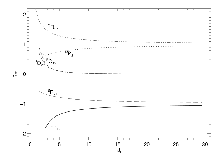
Equation 18 was used to calculate the effective Landé factors of the satellite branches of the CH A${}^{2}\Delta$–X${}^{2}\Pi$ system in the G-band region as a function of the lower-level angular momentum quantum number $J_{l}$ shown in Figure 4. A similar graph is shown by Berdyugina & Solanki (2002, their Fig. 9) for the main branch transitions of the CH molecule. Note that while $g_{\mathrm{eff}}$ for all the main branches tends to zero with increasing $J_{l}$, this is not the case for the those of the ${}^{Q}P_{21}$ and ${}^{Q}R_{12}$, and ${}^{O}P_{12}$ and ${}^{S}R_{21}$ type satellite branches, which tend to $+1$ and $-1$, respectively. Only effective Landé factors of the $Q$ type satellite branches follow the behavior of the main branch transitions. Despite the tendency of $g_{\mathrm{eff}}$ of the $P$ and $R$ satellite branches to $\pm 1$, we found in the calculations described below that the satellite branch lines contribute little to the polarization signal in the G band because they are generally much weaker than the main branch lines as indicated by comparison of Figures 2 and 3.

3 Model calculations

To get a first impression of the feasibility of bright point magnetic field measurement through the Zeeman effect in the CH lines of the G band we calculated the polarization at these wavelengths due to a 0.1 T constant vertical field in a one-dimensional plane-parallel model of the quiet solar atmosphere. In addition, we modeled the polarization signal through a two-dimensional cross section of a snapshot from a three-dimensional solar magneto-convection simulation.

3.1 Radiative transfer

We implemented the rules for energy level splitting in Hund’s case (b) (see eq. [2.1]) and line component strength (Table 1) in a numerical radiative transfer code to calculate the splitting patterns of the CH lines in the G-band region. The code accounts for all components in each of the CH lines and does not rely on the calculated effective Landé factors.

Concentration of the CH molecule in each location of the models was calculated by solving the coupled chemical equilibrium equations of a set of 12 molecules consisting of H₂, H${}_{2}^{+}$, C₂, N₂, O₂, CH, CO, CN, NH, NO, OH, and H₂O, and their atomic constituents. The population of individual CH levels was calculated according to the Saha–Boltzmann equations, so that the molecular line opacity and source function were assumed to be in Local Thermodynamic Equilibrium (LTE). Values of wavelengths and line strengths were taken from file HYDRIDES.ASC of CD-ROM 18 by Kurucz, which results in a similar emergent spectrum as the list provided by Jorgensen et al. (1996), although the latter includes many more weaker lines. In addition, opacities due to background atomic lines were included from files gf0430.10 and gf0440.10 of CD-ROM 1 by Kurucz³. The opacities and source functions of these lines were assumed to be in LTE as well, and for each of the electric dipole transitions among them Zeeman splitting patterns (e.g., Stenflo, 1994, pp. 107-111) were calculated as input for the polarized radiative transfer calculation.

For each wavelength for which the emergent intensity was to be calculated the contributions from molecular and atomic lines to the $4\times 4$ propagation matrix $\mathbf{K}$ and the 4-element Stokes emissivity $\mathbf{e}$ (Trujillo Bueno, 2003b) were added as well as the (unpolarized) contributions from relevant background continuum processes. Given the propagation matrix and emission vector the Stokes transfer equation was solved using the quasi-parabolic DELO method proposed by Trujillo Bueno (2003b, see 2000 for a first application of this method). The DELO method works analogous to the short characteristics method (Kunasz & Auer, 1988; Auer et al., 1994) for unpolarized radiation and is easily generalized to multi-dimensional geometry.

3.2 Plane-parallel atmosphere with imposed magnetic field

Figure 5: Intensity (in units of $10^{-8}$ J m^-2 s^-1 Hz^-1 sr^-1) and Stokes $V$ profiles (in percentage of continuum intensity) in the G-band region. Thick curve is the calculated spectrum accounting for both atomic and molecular CH lines. Dash-dotted line represents spectrum due to CH lines only. Thin curve is the central intensity atlas, the dotted curve represents a typical G-band filter with 1 nm FWHM, and each of the vertical marks indicates the position of a CH line.

To investigate whether the intensity and polarization spectra anywhere in the G band are dominated solely by CH lines we solved the full Stokes radiative transfer equations over a wavelength range of 3 nm centered around 430.50 nm through a one-dimensional hydrostatic model of the average quiet solar atmosphere (FALC, model C of Fontenla et al., 1993) with an imposed vertical magnetic field of 0.1 T (1000 G). The resulting Stokes $I$ and $V$ spectra are given in Figure 5, where the thick solid curves represent the calculated $I$ and $V$ spectra taking account of both the atomic and CH molecular line contributions, and the dash-dotted curves represent the calculated spectra with the contribution from atomic lines omitted. Also plotted in this figure are the transmission curve of a typical G-band filter (dotted curve) with a FWHM of 1 nm and the disk centre solar intensity spectrum (thin solid curve, Kurucz, 1991). Overall, there is good agreement between the calculated intensity spectrum that includes all lines (thick solid curve) and the observed spatially averaged atlas spectrum (thin solid line), indicating that the linelists we use are adequate for our purposes.

Comparison between the solid curve and dash-dotted curves in $I$ and $V$ allows us to locate regions where the spectra are dominated by CH lines alone. We identified the locations at 429.74, 429.79, 430.35 through 430.41, 430.89, 431.19, and 431.35 nm as the possible regions of interest for observations if we want to measure bright point magnetic fields through the Zeeman effect in the CH lines. Typical circular polarization signals at the wavelengths where CH lines alone dominate the spectrum are 2–5% for the 0.1 T constant vertical field compared to 20% for the strongest atomic lines in this region. These predicted values are well within the range of what could be observed with sufficient spatial resolution. None of these regions is dominated by a single CH line, rather the spectrum in each is the result of overlapping lines of varying degrees of magnetic sensitivity. As a result, none of the profiles in Stokes $V$ has a regular double-lobed antisymmetric shape. In particular, the profile around 430.40 nm is notable. The one-lobed profile is the result of two $R_{11}$ main branch lines in the $v=0$ band at 430.3925 and 430.3932 nm with $J_{l}=1.5$ and $J_{u}=2.5$, and $g_{\mathrm{eff}}=0.8833$ that overlap with lines that are much less magnetically sensitive. It raises the interesting possibility of recovering the bright point magnetic field with narrowband imaging in only one polarization, avoiding the difficulties of reconstructing the polarization map from two different exposures. At the low rotational quantum number of the two $R_{11}$ lines the electron spin is not completely decoupled from the inter-nuclear axis and calculation of the effective Landé factors for these transitions has to be treated with the intermediate case (a-b) formalism (Schadee, 1978). Future polarimetry employing these lines would benefit from applying a more precise value of $g_{\mathrm{eff}}$, which according to the graph in Fig. 9 of Berdyugina & Solanki (2002) is about 0.1 higher than the value for pure case (b). In fact, we have verified that performing the synthesis using the Zeeman patterns calculated in the intermediate case (a-b) by means of the formalism developed by Schadee (1978) gives similar results.

3.3 Magneto-convection snapshot

For a prediction of the amount of Zeeman induced polarization under more realistic conditions in the solar photosphere we solved the Stokes transfer equations in a two-dimensional cross section through a simulation of magneto-convection (Stein et al., 2003). In this simulation the physical domain extends 12 Mm in both horizontal directions with a resolution of 96 km, extends 2.5 Mm below the surface, and spans 3 Mm vertically. Periodic boundary conditions were used in the horizontal directions, and transmitting vertical boundary conditions were specified. Radiative contributions to the energy balance were calculated by solving radiative transfer in LTE using a four bin opacity distribution function.

Figure 6: Calculated Stokes $V$ (top) and $I$ spectra for cross section through a magneto-convection snapshot. The polarization signal at wavelengths 430.36 and 430.40 is due the Zeeman effect in CH lines alone.

For the Stokes transfer calculations a two-dimensional cut through a single three-dimensional simulation snapshot was selected. The upper part of this slice, starting at 300 km below the photosphere, was interpolated onto a finer vertical grid, logarithmically in densities, and linearly in temperature and velocities. Through this interpolated cross section the Stokes transfer equations were solved in two-dimensional geometry over a subset of wavelengths centered on 430.4 nm. The snapshot employed for this paper had an average vertical field of 0.003 T.

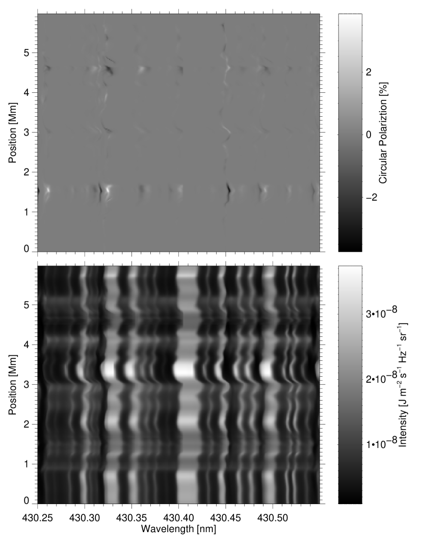
The emergent Stokes $I$ and $V$ spectra from the slice in the wavelength region around 430.40 nm are shown in Figure 6. The polarization signal at wavelengths 430.36 and 430.40 is due to the Zeeman effect in CH lines alone. It is most prominent at positions 1.5, 3.0, and 4.5 Mm. All three of these locations are associated with downflows as deduced from the redshifts in the intensity spectrum, and are probably positioned in intergranular lanes. At positions 1.5 and 4.5 Mm along the slice the line-of-sight component (in the vertical direction) of the field is strongest and results in a circular polarization signal of about 1% of the local continuum intensity. Given the size of these magnetic elements of order 100 km, and if the element is isolated without oposite magnetic polarities within the resolution element, they should produce a polarization signal of order at least $10^{-4}$ even when the (seeing induced) telescope resolution is only of order 1 Mm (corresponding to slightly more than $1^{\prime\prime}$). This is within the capabilities of current polarimetric instrumentation.

It is worth noting that the spectral feature at 430.40 does not consistently show a one-lobed profile as it does in the spectrum produced by the one-dimensional hydrostatic model. In particular, at position 1.5 Mm the blue lobe is visible as well, altough much weaker than its red counterpart. The difference with the hydrostatic model most likely derives through an interplay between the magnetic field and velocity gradients in the dynamic case, and the different formation heights of the magnetically sensitive and non-sensitive lines. This inconsistency would make magnetic field mapping through narrow band imaging in one polarity a less reliable method, but its downside would have to be weighed against the improved spatial resolution this technique promises, including the full benefit it would have from image improving techniques like adaptive optics and post facto image reconstruction.

4 Conclusion

We have solved the full set of Stokes transfer equations in two different models of the solar atmosphere in the wavelength region of the G band around 430 nm. We include polarization due to the Zeeman effect in atomic transitions, and most importantly in the molecular CH lines that are the major contributors to opacity in the G band. Judging from the calculated spectrum through a one-dimensional plane parallel model of the solar atmosphere (FALC) we find several wavelengths regions at which both the intensity and the polarization signals are dominated by CH lines, without significant contribution from atomic lines. The amplitude of the calculated polarization signal in these locations, of order 2–5% in the hydrostatic FALC model with 0.1 T constant vertical field and of the order of 1% of the continuum intensity in Stokes $V$ through the magneto-convection slice, leads us to predict that measurement of field strength in the CH lines that provide small-scale magnetic elements with their characteristic brightness is a realistic prospect.

Because of the property of the lines of the strong CH main branch to become less magnetically sensitive with increasing rotational quantum number (as evidenced by the behavior of their effective Landé factors as shown by Berdyugina & Solanki (2002)) the polarization spectrum of the G band is significantly less crowded than its intensity spectrum. Nevertheless, overlap of lines still occurs and none of the isolated CH features shows a regular symmetric $V$-profile even in the absence of any flows. In this paper we show that the effective Landé factors of the $P$ and $R$ satellite branches go asymptotically $\pm 1$ with increasing molecular rotation (Figure 4). However, these satellite branch transitions are much weaker than their counter parts in the main branches and do not contribute significantly to the polarization signal in the G band.

Within the 3 nm wavelength interval we investigated we found one location where several CH lines overlap and dominate the spectrum to produce a single-lobed $V$-profile at 430.40 nm. In particular, the spectrum calculated through the hydrostatic FALC model shows this behavior, which prompts us to suggest that measurement of bright-point line-of-sight magnetic field strength could be achieved through narrowband (of order 20 pm FWHM or 200 mÅ) imaging in one direction of circular polarization. Such a method would have the full benifit of image quality improving techniques like adaptive optics and phase diversity restoration for optimal spatial resolution. Unfortunately, the $V$ spectrum calculated through the two-dimensional magneto-convection slice shows a very asymmetric two-lobed profile at 430.40 nm in some locations rather than a uniformly single-lobed one. Nonetheless, the benefit of optimal spatial resolution may outweigh the polarimetric accuracy in some cases. Proof that such curious single-lobed $V$-profiles indeed exist in the solar spectrum comes from recent observations of sunspots obtained with the ZIMPOL polarimeter attached to the Gregory Coudé telescope of IRSOL (locarno), which will be discussed in an upcoming paper.

We conclude that the technique of magnetic field measurement through Stokes polarimetry of the CH lines finally holds the promise for the development of a method that will allow us to unambiguously determine what the role of the field is in the appearance of G-band bright points. If such measurements are successful we will no longer have to deal with the difficulty of interpreting magnetic field measurements in atomic lines together with G-band intensity measurements introduced by the different formation properties of these species.

References

- Asensio Ramos & Trujillo Bueno (2003) Asensio Ramos, A., & Trujillo Bueno, J. 2003, in J. Trujillo Bueno, J. Sánchez Almeida (eds.), Solar Polarization 3, ASP Conf. Series Vol. 307, The Astronomical Society of the Pacific, San Francisco, CA, p. 195
- Auer et al. (1994) Auer, L., Fabiani Bendicho, P., & Trujillo Bueno, J. 1994, A&A, 292, 599
- Berdyugina et al. (2000) Berdyugina, S. V., Frutiger, C., Solanki, S. K., & Livingston, W. 2000, A&A, 364, L101
- Berdyugina & Solanki (2002) Berdyugina, S. V., & Solanki, S. K. 2002, A&A, 385, 701
- Berger et al. (1995) Berger, T. E., Schrijver, C. J., Shine, R. A., Tarbell, T. D., Title, A. M., & Scharmer, G. 1995, ApJ, 454, 531
- Berger & Title (2001) Berger, T. E., & Title, A. M. 2001, ApJ, 553, 449
- Brink & Satchler (1968) Brink, D. M., & Satchler, G. R. 1968, Angular Momentum, 2nd edition, Clarendon Press, Oxford
- Chapman & Sheeley (1968) Chapman, G. A., & Sheeley, N. R. 1968, Solar Phys., 5, 442
- Dunn & Zirker (1973) Dunn, R. B., & Zirker, J. B. 1973, Solar Phys., 33, 281
- Fontenla et al. (1993) Fontenla, J. M., Avrett, E. H., & Loeser, R. 1993, ApJ, 406, 319
- Fraunhofer (1817) Fraunhofer, J. 1817, Denkschriften der Münch. Akad. der Wissenschaften, 5, 193
- Herzberg (1950) Herzberg, G. 1950, Molecular Spectra and Molecular Structure I. Spectra of Diatomic Molecules, D. van Nostrand Company, Inc., New York
- Jorgensen et al. (1996) Jorgensen, U. G., Larsson, M., Iwamae, A., & Yu, B. 1996, A&A, 315, 204
- Kunasz & Auer (1988) Kunasz, P. B., & Auer, L. H. 1988, J. Quant. Spectrosc. Radiat. Transfer, 39, 67
- Kurucz (1991) Kurucz, R. L. 1991, in A. Cox, W. Livingston, M. Matthews (eds.), Solar interior and atmosphere, University of Arizona Press, Tucson, AZ, p. 663
- Landi Degl’Innocenti (2003) Landi Degl’Innocenti, E. 2003, in J. Trujillo Bueno, J. Sánchez Almeida (eds.), Solar Polarization 3, ASP Conf. Series Vol. 307, The Astronomical Society of the Pacific, San Francisco, CA, p. 164
- Langhans et al. (2001) Langhans, K., Schmidt, W., Rimmele, T., & Sigwarth, M. 2001, in M. Sigwarth (ed.), Advanced Solar Polarimetry – Theory, Observation, and Instrumentation, ASP Conf. Ser., Vol. 236, The Astronomical Society of the Pacific, San Francisco, CA, p. 439
- Mehltretter (1974) Mehltretter, J. P. 1974, Solar Phys., 38, 43
- Muller (1985) Muller, R. 1985, Solar Phys., 100, 237
- Muller et al. (2000) Muller, R., Dollfus, A., Montagne, M., Moity, J., & Vigneau, J. 2000, A&A, 359, 373
- Muller et al. (1989) Muller, R., Hulot, J. C., & Roudier, T. 1989, Solar Phys., 119, 229
- Muller & Roudier (1992) Muller, R., & Roudier, T. 1992, Solar Phys., 141, 27
- Muller et al. (1994) Muller, R., Roudier, T., Vigneau, J., & Auffret, H. 1994, A&A, 283, 232
- Rutten et al. (2001) Rutten, R. J., Kiselman, D., Rouppe van der Voort, L., & Plez, B. 2001, in M. Sigwarth (ed.), Advanced Solar Polarimetry – Theory, Observation, and Instrumentation, ASP Conf. Ser., Vol. 236, The Astronomical Society of the Pacific, San Francisco, CA, p. 445
- Sánchez Almeida et al. (2001) Sánchez Almeida, J., Asensio Ramos, A., Trujillo Bueno, J., & Cernicharo, J. 2001, ApJ, 555, 978
- Schadee (1978) Schadee, A. 1978, Journal of Quantitative Spectroscopy and Radiative Transfer, 19, 517
- Sheeley (1971) Sheeley, N. R. 1971, Solar Phys., 20, 19
- Slater (1960) Slater, J. C. 1960, Quantum Theory of Atomic Structure, McGraw-Hill Book Company, Inc., New York
- Socas Navarro et al. (2000) Socas Navarro, H., Trujillo Bueno, J., & Ruiz Cobo, B. 2000, ApJ, 530, 977
- Spruit & Zwaan (1981) Spruit, H. C., & Zwaan, C. 1981, Solar Phys., 70, 207
- Stein et al. (2003) Stein, R. F., Bercik, D., & Nordlund, A. 2003, in A. A. Pevtsov, H. Uitenbroek (eds.), Current Theoretical Models and High Resolution Solar Observations: Preparing for ATST, ASP Conf. Ser., Vol. 286, The Astronomical Society of the Pacific, San Francisco, CA, p. 121
- Steiner et al. (2001) Steiner, O., Hauschildt, P. H., & Bruls, J. 2001, A&A, 372, L13
- Stenflo (1973) Stenflo, J. O. 1973, Solar Phys., 32, 41
- Stenflo (1994) Stenflo, J.-O. 1994, Solar Magnetic Fields. Polarized Radiation Diagnostics, Kluwer Academic Publishers, Dordrecht
- Trujillo Bueno (2003a) Trujillo Bueno, J. 2003a, in J. Trujillo Bueno, J. Sánchez Almeida (eds.), Solar Polarization 3, ASP Conf. Series Vol. 307, The Astronomical Society of the Pacific, San Francisco, CA, p. 407
- Trujillo Bueno (2003b) Trujillo Bueno, J. 2003b, in I. Hubeny, D. Mihalas, K. Werner (eds.), Stellar Atmosphere Modeling, ASP Conf. Ser., Vol. 288, The Astronomical Society of the Pacific, San Francisco, CA, p. 551
- Uitenbroek (2003) Uitenbroek, H. 2003, in A. A. Pevtsov, H. Uitenbroek (eds.), Current Theoretical Models and High Resolution Solar Observations: Preparing for ATST, ASP Conf. Ser., Vol. 286, The Astronomical Society of the Pacific, San Francisco, CA, p. 404
- van Ballegooijen et al. (1998) van Ballegooijen, A. A., Nisenson, P., Noyes, R. W., Löfdahl, M. G., Stein, R. F., Nordlund, Å., & Krishnakumar, V. 1998, ApJ, 509, 435