Time-dependent evolution of quasi-spherical, self-gravitating accretion flow

Abstract

A self-similar solution for time evolution of quasi-spherical, self-gravitating accretion flows is obtained under the assumption that the generated heat by viscosity is retained in the flow. The solutions are parameterized by the ratio of the mass of the accreting gas to the central object mass and the viscosity coefficient. While the density and the pressure are obtained simply by solving a set of ordinary differential equations, the radial and the rotational velocities are presented analytically. Profiles of the density and the rotational velocities show two distinct features. Low density outer accreting flow with relatively flat rotation velocity, surrounds an inner high density region. In the inner part, the rotational velocity increases from the center to a transition radius where separates the inner and outer portions. We show that the behaviour of the solutions in the inner region depends on the ratio of the heat capacities, $\gamma$, and the viscosity coefficient, $\alpha$.

1 Introduction

Accretion processes are now believed to play a major role in many astrophysical objects, from protostars to disks around compact stars and AGN. Such systems have been studied at different levels depending on their physical properties. Geometry of the disk (thin or thick), transport of the thermal energy inside the disk, self-gravity of the accreting gas and the magnetic fields are among the most important factors which shape any theory for such systems. For simplicity, traditional models of accretion disks assume geometrically thin configuration and neglect self-gravity of the accreting material (Shakura and Sunyaev 1973; Pringle 1981). These models have been extended by considering large scale magnetic fields, polytropic equation of state and better understanding of the mechanism of angular momentum transport (e.g., Livio and Pringle 1992; Ogilvie 1997; Duschl, Strittmatter and Biermann 2000). However, the key ingredient in all such models is that the generated heat by turbulent viscosity does not remain in the flow. In other words, all of the viscously dissipated energy was assumed to be radiated away immediately.

Another type of accretion flow known as Advection-Dominated Accretion Flow (ADAF) has been proposed, in which generated heat by viscosity can not escape from the system and retains in the flow (Ichimaru 1977; Narayan and Yi 1994). During recent years, ADAFs have been paid attention as plausible states of accretion flows around black holes, active galactic nuclei or dim galactic nuclei (for review see Kato, Fukue and Mineshige 1998). Using similarity method, Ogilvie (1999) (hereafter; OG) extended original steady state self-similar solutions to time dependent case. His solutions describe quasi-spherical time dependent advection dominated accretion flows.

On the other hand, many authors tried to study the effects related to the disk self-gravity. Recent observations show significant deviations from Keplerian rotation in objects that are believed to be accretion disk, and in some cases, there are strong evidences that the amount of mass in the disk is large (e.g., Drimmel 1996; Greenhill 1996). The role of self-gravity in accretion disks was discussed by Paczyński (1978), who studied vertical structure of the disk under the influence of self-gravity. Some authors investigated role of self-gravity on waves in the disk (Lin and Pringle 1987; Lin and Pringle 1990). Within the framework of geometrically thin configuration, Mineshige and Umemura (1996) extended classical self-similar ADAF solution (Narayan and Yi 1994) and found a global one dimensional disk solutions influenced by self-gravity both in the radial and perpendicular directions to the disk. In another study, Mineshige and Umemura (1997) extended previous steady solutions to the time dependent case while the effect of self-gravity of the disk had been taken into account. They used isothermal equation of state and so their solutions describe a viscous accretion disk in slow accretion limit. Then, Mineshige, Nakayma and Umemura (1997) extended this study by obtaining solutions for polytropic viscous accretion disks. Also, Tsuribe (1999) studied self-similar collapse of an isothermal viscous accretion disk.

Although solution of Mineshige and Umemura (1996) describes self-gravitating ADAFs, applicability of the solution restricts to geometrically thin configurations. The most appropriate geometrical configuration for advective flows, rather than thin, is quasi-spherical as has been confirmed by many authors (e.g, Narayan and Yi 1995). OG presented the first semi-analytical quasi-spherical, time-dependent ADAFs solution. Here we note that although OG considered advection-dominated accretion flow in a point mass potential, it is straightforward to relax this assumption so as to describe the effect of self-gravitation on quasi-spherical advection-dominated accretion flows using time-dependent similarity solutions.

This paper is organized as follows. In section 2 the general problem of constructing a model for quasi-spherical, self-gravitating accretion flow is defined. The self-similar solutions are presented in section 3, and the effects of the input parameters are examined. We summarize the results in section 4.

2 Formulation of the Problem

We start with the approach adopted by Ogilvie (1999) who studied quasi-spherical accretion flow without self-gravity. In his approach, the equations are written in spherical coordinates $(r,\theta,\varphi)$ by considering the equatorial plane $\theta=\frac{\pi}{2}$ and neglecting terms with any $\theta$ and $\varphi$ dependence. It implies that each physical variable represents approximately spherically averaged quantity. So, all the physical quantities depend only on the spherical radius $r$ and time $t$. Self-gravity of the accreting gas can be considered simply by Poisson equation and the corresponding term in the momentum equation. The governing equations are the continuity Equation,

$$\frac{\partial\rho}{\partial t}+\frac{1}{r^{2}}\frac{\partial}{\partial r}(r^{2}\rho v_{\rm r})=0,{}$$ (1)

the Equations of motion,

$$\frac{\partial v_{\rm r}}{\partial t}+v_{\rm r}\frac{\partial v_{\rm r}}{\partial r}+\frac{1}{\rho}\frac{\partial p}{\partial r}+\frac{\partial\Psi}{\partial r}+\frac{GM_{\star}}{r^{2}}=\frac{v_{\rm\varphi}^{2}}{r},$$ (2)

$$\rho(\frac{\partial}{\partial t}(rv_{\rm\varphi})+v_{\rm r}\frac{\partial}{\partial r}(rv_{\rm\varphi}))=\frac{1}{r^{2}}\frac{\partial}{\partial r}[\nu\rho r^{4}\frac{\partial}{\partial r}(\frac{v_{\rm\varphi}}{r})],$$ (3)

the Poisson’s Equation,

$$\frac{1}{r^{2}}\frac{\partial}{\partial r}(r^{2}\frac{\partial\Psi}{\partial r})=4\pi G\rho,$$ (4)

and the energy Equation,

$$\frac{1}{\gamma-1}(\frac{\partial p}{\partial t}+v_{\rm r}\frac{\partial p}{\partial r})+\frac{\gamma}{\gamma-1}\frac{p}{r^{2}}\frac{\partial}{\partial r}(r^{2}v_{\rm r})=\nu\rho r^{2}[\frac{\partial}{\partial r}(\frac{v_{\rm\varphi}}{r})]^{2}.$$ (5)

In order to solve the equations, we need to assign the kinematic coefficient of viscosity $\nu$. Although there are many uncertainties about the exact form of viscosity, authors introduce some prescriptions for $\nu$ regarding dimensional analysis or just based on phenomenological considerations (e.g, Duschl, Strittmatter and Biermann 2000). We employ the usual $\alpha$ prescription for the viscosity, which we write as (Shakura and Sunyaev 1973)

$$\nu=\alpha\frac{p}{\rho\Omega_{\rm k}},$$ (6)

where $\Omega_{\rm k}=(GM_{\star}/r^{3})^{1/2}$ is the Keplerian angular velocity at radius $r$. This prescription originally introduced for viscosity in thin accretion disk, however, it has been widely used for studying dynamics of thick accretion disk, such as ADAFs.

To simplify the equations, we make the following substitutions:

$$\rho\rightarrow\hat{\rho}\rho,p\rightarrow\hat{p}p,v_{r,\varphi}\rightarrow\hat{v}v_{r,\varphi},\Psi\rightarrow\hat{\Psi}\Psi,r\rightarrow\hat{r}r,t\rightarrow\hat{t}t,$$ (7)

where

$$\hat{v}=\sqrt{\frac{GM_{\star}}{\hat{r}}}=\frac{\hat{r}}{\hat{t}},\hat{t}=\frac{1}{\sqrt{4\pi G\hat{\rho}}},\hat{p}=\hat{\rho}\hat{v}^{2},\hat{\Psi}=\frac{GM_{\star}}{\hat{r}}.$$ (8)

Under these transformation, the continuity equation does not change and the rest of equations are cast into

$$\frac{\partial v_{\rm r}}{\partial t}+v_{\rm r}\frac{\partial v_{\rm r}}{\partial r}+\frac{1}{\rho}\frac{\partial p}{\partial r}+\frac{\partial\Psi}{\partial r}+\frac{1}{r^{2}}=\frac{v_{\rm\varphi}^{2}}{r},{}$$ (9)

$$\rho(\frac{\partial}{\partial t}(rv_{\rm\varphi})+v_{\rm r}\frac{\partial}{\partial r}(rv_{\rm\varphi}))=\frac{\alpha}{r^{2}}\frac{\partial}{\partial r}[pr^{11/2}\frac{\partial}{\partial r}(\frac{v_{\rm\varphi}}{r})],$$ (10)

$$\frac{1}{r^{2}}\frac{\partial}{\partial r}(r^{2}\frac{\partial\Psi}{\partial r})=\rho,{}$$ (11)

$$\frac{1}{\gamma-1}(\frac{\partial p}{\partial t}+v_{\rm r}\frac{\partial p}{\partial r})+\frac{\gamma}{\gamma-1}\frac{p}{r^{2}}\frac{\partial}{\partial r}(r^{2}v_{\rm r})=\alpha pr^{7/2}[\frac{\partial}{\partial r}(\frac{v_{\rm\varphi}}{r})]^{2}.{}$$ (12)

3 Self-Similar Solutions

We look for self-similar solutions of Equations (1) and (9)-(12) and reduce this system into a set of ordinary differential equations. We define a self-similar variable

$$\xi=\frac{r}{(t_{0}-t)^{2/3}},$$ (13)

where $t<t_{\rm 0}$ and demand that

$$\rho(r,t)=(t_{0}-t)^{-2}R(\xi),$$ (14)

$$\ p(r,t)=(t_{0}-t)^{-8/3}P(\xi),$$ (15)

$$\ v_{\rm r}(r,t)=(t_{0}-t)^{-1/3}V(\xi),$$ (16)

$$\ v_{\rm\varphi}(r,t)=(t_{0}-t)^{-1/3}\Phi(\xi),$$ (17)

$$\Psi(r,t)=(t_{0}-t)^{-2/3}S(\xi).$$ (18)

Substituting these expressions into the above Equations, we obtain the following set of self-similar Equations:

$$\ -\frac{2}{9}\xi+\frac{1}{R}\frac{dP}{d\xi}+\frac{dS}{d\xi}+\frac{1}{\xi^{2}}=\frac{\Phi^{2}}{\xi},$$ (19)

$$\ -\xi^{3}R(\Phi+2\xi\frac{d\Phi}{d\xi})=3\alpha\frac{d}{d\xi}[P\xi^{11/2}\frac{d}{d\xi}(\frac{\Phi}{\xi})],$$ (20)

$$\frac{1}{\xi^{2}}\frac{d}{d\xi}(\xi^{2}\frac{dS}{d\xi})=R,$$ (21)

$$\frac{2}{3}(\frac{4-3\gamma}{\gamma-1})=\alpha\xi^{7/2}[\frac{d}{d\xi}(\frac{\Phi}{\xi})]^{2}.{}$$ (22)

Interestingly, the continuity Equation is integrable and gives $\xi^{2}R(\xi+3V/2)=C$, where $C$ is a constant and should be zero. Thus,

$$\ V=-\frac{2}{3}\xi.$$ (23)

Also, we can obtain rotational similarity function $\Phi(\xi)$ simply by integrating Equation (22),

$$\Phi(\xi)=\frac{\xi}{\xi_{\rm s}}\Phi_{s}+\frac{4\lambda}{3}(\xi^{1/4}-\xi_{\rm s}^{-3/4}\xi).{}$$ (24)

where

$$\lambda=\sqrt{\frac{2}{3\alpha}(\frac{4-3\gamma}{1-\gamma})},$$ (25)

and $\Phi_{\rm s}$ is rotational velocity at some $\xi_{\rm s}$. For simplicity, we assume that $\xi_{\rm s}$ defines the outer boundary of the accretiong gas. This Equation correctly gives $\Phi(\xi=0)=0$, and reaches to a maximum $\Phi_{\rm m}$ by increasing $\xi$ from zero to a point at $\xi_{\rm m}$. One can simply show

$$\xi_{\rm m}=\frac{1}{4\sqrt[3]{4}}(\frac{\xi_{\rm s}}{\sqrt[4]{\xi_{\rm s}}-\sqrt[4]{\xi_{\rm 0}}})^{4/3},$$ (26)

where $\xi_{\rm 0}=3\Phi_{\rm s}/4\lambda$ and

$$\Phi_{\rm m}=\frac{\lambda}{\sqrt[3]{4}}(\frac{\xi_{\rm s}}{\sqrt[4]{\xi_{\rm s}}-\sqrt[4]{\xi_{\rm 0}}})^{1/3}.$$ (27)

Clearly, behaviour of rotational velocity and the other physical variables except for the radial velocity, depend on $\xi_{\rm s}$ and $\Phi_{\rm s}$. We can consider both $\xi_{\rm s}$ and $\Phi_{\rm s}$ as free parameters, however, it’s possible to determine them uniquely, if we parameterize self-similar solutions using conserved quantities, e.g. mass of the system. As can be seen from the definition of $\lambda$, the above self-similar solutions are applicable within the range of $1<\gamma<4/3$ if we consider a positive value for $\alpha$.

We can derive asymptotic solutions when approaching the origin $\xi=0$ as follows

$$\Phi(\xi)\longrightarrow\frac{4}{3}\lambda\xi^{1/4},$$ (28)

$$\ R(\xi)\longrightarrow 4(\frac{2}{3}\lambda^{2}+\frac{1}{11\alpha})\xi^{-3/2},$$ (29)

$$\ P(\xi)\longrightarrow\frac{32}{33\alpha}(\frac{2}{3}\lambda^{2}+\frac{1}{11\alpha})\xi^{-1}.$$ (30)

These asymptotic solutions are valuable when performing numerical integrations to obtain similarity solutions starting from $x\rightarrow 0^{+}$. Note that the behaviour of the solutions near to origin only depends on $\lambda$ and $\alpha$.

We now proceed to solve the rest of above similarity Equations. By substituting Equation (24) into Equation (20), we obtain

$$\frac{15}{4}P+\xi\frac{dP}{d\xi}=f(\xi)R.$$ (31)

where

$$f(\xi)=\frac{\xi^{1/4}}{3\alpha\lambda}[3\frac{\Phi_{\rm s}}{\xi_{\rm s}}\xi+4\lambda(\frac{1}{2}\xi^{1/4}-\xi_{\rm s}^{-3/4}\xi)].$$ (32)

After some algebra, from this Equation and Equations (19) and (21), the following Equation is obatined:

$$\frac{15}{4}fP\frac{d^{2}P}{d\xi^{2}}=S_{1}(\xi,P,dP/d\xi)+S_{2}(\xi,P,dP/d\xi)+S_{3}(\xi,P,dP/d\xi),$$ (33)

where

$$S_{1}=\frac{19}{4}f(\frac{dP}{d\xi})^{2}-(\frac{df}{d\xi})(\frac{dP}{d\xi})(\frac{15}{4}P+\xi\frac{dP}{d\xi}),$$ (34)

$$S_{2}=\frac{g}{\xi^{2}}(\frac{15}{4}P+\xi\frac{dP}{d\xi})^{2}-\frac{1}{f}(\frac{15}{4}P+\xi\frac{dP}{d\xi})^{3},$$ (35)

$$S_{3}=-2\frac{f}{\xi}\frac{dP}{d\xi}(\frac{15}{4}P+\xi\frac{dP}{d\xi}),$$ (36)

$$g(\xi)=\frac{d}{d\xi}(\frac{2}{9}\xi^{3}+\xi\Phi^{2}).$$ (37)

This Equation can easily be integrated considering appropriate boundary conditions. We can parameterize the solutions by $\xi_{\rm s}$ as a function of the mass of the accreting gas and the viscosity parameter $\alpha$. For simplicity, we assume $R(\xi_{\rm s})=R_{\rm s}$ and $P(\xi_{\rm s})=P_{\rm s}$. Total mass of the accreting gas is

$$M=4\pi\int_{0}^{\infty}\rho r^{2}dr.$$ (38)

Using similarity solutions, this Equation reads

$$M=M_{\star}\int_{0}^{\xi_{\rm s}}R\xi^{2}d\xi.$$ (39)

Substituting from Poisson Equation (21), we have

$$M=M_{\star}\xi_{\rm s}^{2}\frac{dS}{d\xi}|_{\xi_{\rm s}},$$ (40)

By inserting $dS/d\xi$ from Equation (19) into the above Equation, we finally obtain

$$M=M_{\star}[\xi_{\rm s}\Phi_{\rm s}^{2}+\frac{2}{9}\xi_{\rm s}^{3}-\frac{\xi_{\rm s}^{2}}{R_{\rm s}}(\frac{dP}{d\xi})_{\rm s}-1].$$ (41)

Another relation is obtained from Equation (31), as follows

$$\frac{15}{4}P_{\rm s}+\xi_{\rm s}(\frac{dP}{d\xi})_{\rm s}=f(\xi_{\rm s})R_{\rm s},$$ (42)

where

$$f(\xi_{\rm s})=\frac{\sqrt[4]{\xi_{\rm s}}}{3\alpha\lambda}(3\Phi_{\rm s}-2\lambda\sqrt[4]{\xi_{\rm s}}).$$ (43)

Now, we can use the standard fourth-order Runge-Kutta scheme to integrate nonlinear ordinary differential equation (33) from sufficiently small $\xi$ to $\xi_{\rm s}$. Given $\xi_{\rm s}$ and $\Phi_{\rm s}$ and using asymptotic solutions near to the origin (i.e., equations (29) and (30)), one can start numerical integration and equation (41) gives corresponding ratio of masses, i.e. $M/M_{\star}$. Before presenting results of integration, it would be interesting to explore the typical behaviour of rotational velocity $\Phi(\xi)$.

Just as an illustrative example we follow another approach: lets assume that we know $R_{\rm s}$, $P_{\rm s}$ and $M/M_{\star}$ from numerical integration and so, one can determine $\xi_{\rm s}$ and $\Phi_{\rm s}$ from Equations (41) and (42) uniquely. For example, if we set $P_{\rm s}=0$ and $(dP/d\xi)_{\rm s}=0$ and consider non-zero but negligible $R_{\rm s}$, the outer boundary of the system is determined analytically

$$\xi_{\rm s}=\sqrt[3]{2\lambda^{4}+4.5(\frac{M}{M_{\star}}+1)-\sqrt{4\lambda^{4}(\lambda^{4}+4.5(\frac{M}{M_{\star}}+1))}},$$ (44)

and

$$\Phi_{\rm s}=\frac{2}{3}\lambda\sqrt[4]{\xi_{\rm s}}.$$ (45)

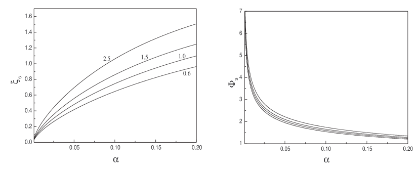
Figure 1: Typical behaviour of $\xi_{\rm s}$ and $\Phi_{\rm s}$ as a function of $\alpha$ corresponding to $\gamma=5/4$, $P_{\rm s}=0$ and $R_{\rm s}\simeq 0$. Left: Each curve is marked by the ratio of mass of the accreting gas to the mass of the central object, $M/M_{\star}$. Right: While the lowest curve corresponds to $M/M_{\star}=0.6$, the curve shifts upward as this ratio increases.

In this case, Figure 1 shows $\xi_{\rm s}$ and $\Phi_{\rm s}$ as functions of $\alpha$ for $\gamma=5/4$ and $M/M_{\star}=0.6,1,1.5$ and $2.5$. As this Figure shows for fixed ratio of masses, the outer radius of the system increases by increasing the viscosity coefficient $\alpha$. Also, if the ratio of masses increases, the outer radius increases irrespective of the exact value of $\alpha$. However, rotational velocity at $\xi_{\rm s}$ (i.e. $\Phi_{\rm s}$) is not very sensitive to values of $\alpha$ or $M/M_{\star}$ for large values of $\alpha$. If the viscosity coefficient $\alpha$ tends to small values, on the other hand, the rotational velocity $\Phi_{\rm s}$ increases significantly.

In Figure 2, we plot rotational velocity of representative cases with $\alpha=0.01,0.1$ and $M/M_{\star}=0.6,1.5,2.5$. As this Figure shows, rotation of the flow increases from the center to the outer radius. There are two regimes as rotation of the flow concerns. While in the outer part, profile of the rotational velocity in similarity space is nearly flat, in the inner portion this velocity strongly increases. However, for low values of $\alpha$ (e.g. $0.01$), rotational velocity reaches to a maximum then with nearly constant and small slope decreases. Also, the rotational velocity increases as the parameter $\alpha$ decreases and the outer region with flat rotation profile becomes larger, as the ratio of the mass of the accreting gas to the mass of the central object increases. In other words, while rotational behaviour of the inner part is nearly independent of the ratio of masses, the outer portion’s rotation and it’s extension are sensitive to that ratio.

In Figure 3, typical behaviour of the density and the pressure in similarity space are shown. We can see in the inner region the solutions can clearly be described by asymptotic solutions (29) and (30), however, outer region has different density and pressure profiles. Interestingly, behaviour of solutions in the inner region is independent of the extension of the system ($\xi_{\rm s}$) and the rotational velocity $\Phi_{\rm s}$. As the ratio of $M/M_{\star}$ increases, the extension of the outer region becomes larger. Flows with large values of $\alpha$ have lower central mass concentration comparing to accretions with low values of $\alpha$. Generally, one can say quasi-spherical, self-gravitating accretion flows of our model consist of two parts, one inner portion with high density and an outer part with nearly lower density and flat rotation profile. However, in both regions the radial velocity is the same, irrespective of the input parameters.

From Equations (16) and (17), we can simply show that the ratio of the radial velocity to the rotational velocity is $v_{\rm r}(r,t)/v_{\rm\varphi}(r,t)=V/\Phi$. Figure 4 shows this ratio for $\alpha=0.1$ and $0.01$ and three different values of $M/M_{\star}$. Clearly, this ratio of velocities are much smaller than unity, implying that at each radius $r$ and at any time $t$, rotational velocity is greater than the radial velocity. However, as the viscosity parameter $\alpha$ increases, the ratio increases as well. This behaviour is easy to understand; because we showed that radial similarity velocity $V$ is proportional to similarity variable $\xi$, independent of the input parameters. However, rotational similarity velocity $\Phi$ decreases by increasing the parameter $\alpha$, as can be seen from Figure 2. So, the ratio $V/\Phi$ increases in the case that $\alpha$ increases.

As we showed the total mass of the accreting gas is conserved. We can simply write the integral representing the angular momentum as $J=4\pi\int\rho v_{\rm\varphi}r^{3}dr$. Using the similarity solutions, we can show that the total angular momentum $J$ is proportional to $(t_{0}-t)^{1/3}$. In non-self-gravitating quasi-spherical accretion flow, $J$ is conserved and the total mass $M$ is proportional to $(t_{0}-t)^{-1/3}$ as has been shown by OG. But our solutions imply that the total mass of accreting material is conserved and angular momentum is decreasing. Also, the central density $\rho_{\rm c}$ increases as $\rho_{\rm c}\propto(t_{0}-t)^{-2}$. For non-self-gravitating flow, we see another behaviour: $\rho_{\rm c}\propto(t_{0}-t)^{-7/3}$. However, the radius of the flow in both cases decreases in proportion to $(t_{0}-t)^{2/3}$.

4 Summary

In this paper, we have studied quasi-spherical accretion flow, in which heat generated by viscosity retained in the flow. In opposition to the usual studies performed up to now, we have considered self-gravity of the flow. We derived similarity solutions for such flows which are applicable within the range $0<\gamma<4/3$, if we consider positive value of $\alpha$. Radial and rotational velocities have been obtained analytically. Obtained solutions parameterized by the ratio of the disk mass to the central object mass, $M/M_{\star}$, and the viscosity parameter, $\alpha$. We showed that the extension of the accreting gas depends on this ratio and the viscosity parameter. More importantly, these input parameters have direct effect on the rotational velocity.

Our solutions are different from the solutions by OG in various respects. We found that the radial similarity velocity is in proportion to $\xi$, implying no critical point. This fortunate circumstance let us to integrate rest of the Equations simply, although physically one should bear in mind this kind of velocity (i.e., independent of input parameters) is as a result of mathematical limitations of similarity method. At the outer edge of the accreting gas, the density and the pressure have low values comparing to the central region.

Other viscosity laws have been proposed, for instance the $\beta$-prescription which is based on analogy with turbulence observed in laboratory sheared flows and gives $\nu\propto v_{\rm\varphi}r$ (Duschl, Strittmatter and Biermann 2000). Although we have not explored self-gravitating accretion with this prescription, there are self-similar solutions with similarity indices the same as those have been found with $\alpha$-prescription in this paper. However, ordinary differential equations governing the similarity physical variables are different and should be solved numerically. It would be interesting one compare the similarity solutions with $\beta$-prescription with those we have obtained here.

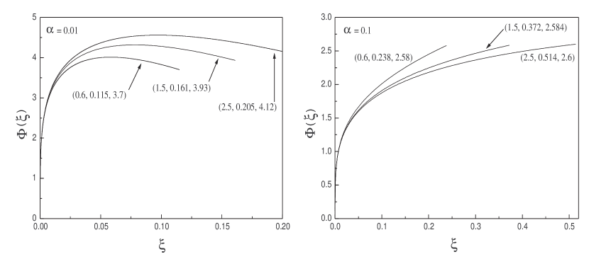
Figure 2: Self-similar rotational velocity corresponding to $\gamma=5/4$ and $R_{\rm s}=P_{\rm s}=0.01$. Each curve is marked by the ratio of the mass of accreting gas to the mass of the central object, $M/M_{\star}$, and $\xi_{\rm s}$ and $\Phi_{\rm s}$ as $(M/M_{\star},\xi_{\rm s},\Phi_{\rm s})$.

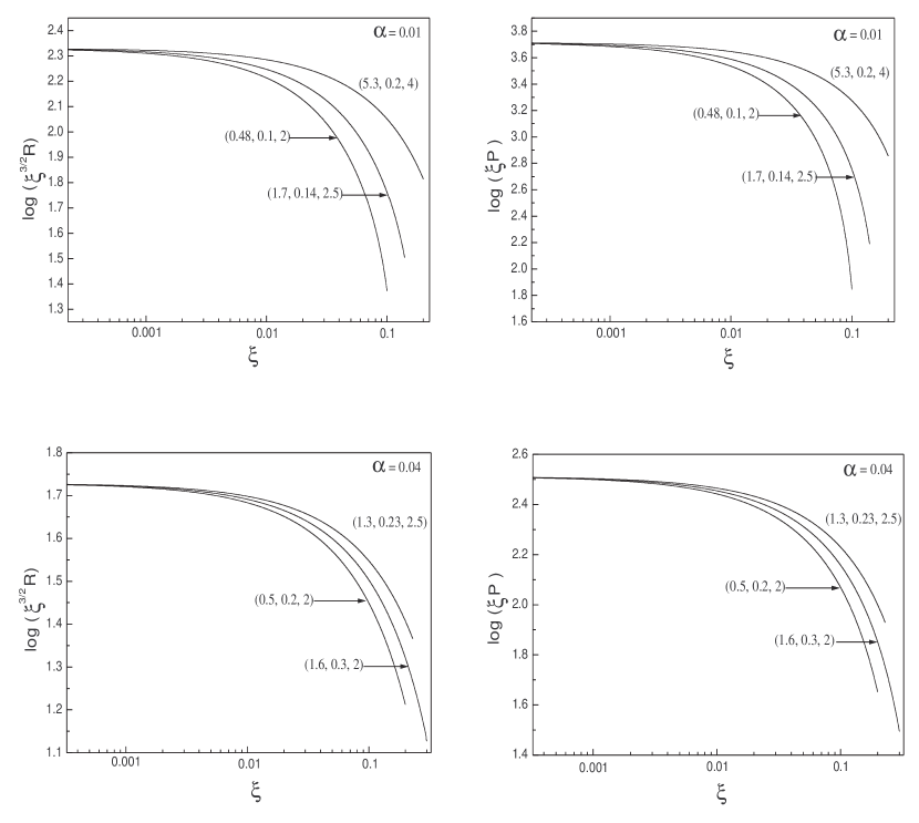
Figure 3: Self-similar density and the pressure corresponding to $\gamma=5/4$ for different values of viscosity coefficient, i.e. $\alpha=0.01$ and $0.04$. Curves are labeled the same as Figure 2.

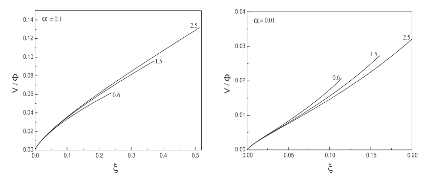
Figure 4: Ratio of the radial velocity to the rotational velocity for $\gamma=5/4$ and $R_{\rm s}=P_{\rm s}=0.01$ and $\alpha=0.1,0.01$. Curves are labeled by the ratio of the masses, i.e. $M/M_{\star}$