Thermal conduction in cosmological SPH simulations

Abstract

Thermal conduction in the intracluster medium has been proposed as a possible heating mechanism for offsetting central cooling losses in rich clusters of galaxies. However, because of the coupled non-linear dynamics of gas subject to radiative cooling and thermal conduction, cosmological hydrodynamical simulations are required to reliably predict the effects of heat conduction on structure formation. In this study, we introduce a new formalism to model conduction in a diffuse ionised plasma using smoothed particle hydrodynamics (SPH), and we implement it in the parallel TreePM/SPH-code GADGET-2. We consider only isotropic conduction and assume that magnetic suppression can be described in terms of an effective conductivity, taken as a fixed fraction of the temperature-dependent Spitzer rate. We also account for saturation effects in low-density gas. Our formulation manifestly conserves thermal energy even for individual and adaptive timesteps, and is stable in the presence of small-scale temperature noise. This allows us to evolve the thermal diffusion equation with an explicit time integration scheme along with the ordinary hydrodynamics. We use a series of simple test problems to demonstrate the robustness and accuracy of our method. We then apply our code to spherically symmetric realizations of clusters, constructed under the assumptions of hydrostatic equilibrium and a local balance between conduction and radiative cooling. While we confirm that conduction can efficiently suppress cooling flows for an extended period of time in these isolated systems, we do not find a similarly strong effect in a first set of clusters formed in self-consistent cosmological simulations. However, their temperature profiles are significantly altered by conduction, as is the X-ray luminosity.

1 Introduction

Clusters of galaxies provide a unique laboratory to study structure formation and the material content of the Universe, because they are not only the largest virialized systems but are also believed to contain a fair mixture of cosmic matter. Among the many interesting aspects of cluster physics, their X-ray emission takes a particularly prominent role. It provides direct information on the thermodynamic state of the diffuse intracluster gas, which makes up for most of the baryons in clusters.

While the bulk properties of this gas are well understood in terms of the canonical $\Lambda$CDM model for structure formation, there are a number of discrepancies between observations and the results of present hydrodynamical simulations. For example, a long standing problem is to understand in detail the scaling relations of observed clusters, which deviate significantly from simple self-similar predictions. In particular, poor clusters of galaxies seem to contain gas of higher entropy in their centres than expected (Ponman et al., 1999; Lloyd-Davies et al., 2000). This has been interpreted either to be evidence for an entropy injection due to non-gravitational processes (Loewenstein, 2000; Wu et al., 1999; Metzler & Evrard, 1994), or as a sign of the selective removal of low-entropy gas by gas cooling (Voit et al., 2002; Wu & Xue, 2002). Both processes combined could influence the thermodynamic properties of the ICM in a complex interplay (Tornatore et al., 2003; Borgani et al., 2003).

Another interesting problem occurs for the radial temperature profiles of clusters. Most observed clusters show a nearly isothermal temperature profile, often with a smooth decline in their central parts (Allen et al., 2001; Johnstone et al., 2002; Ettori et al., 2002). Nearly isothermal profiles are also obtained in adiabatic simulations of cluster formation (e.g. Frenk et al., 1999). However, clusters in simulations that include dissipation typically show temperature profiles that increase towards the centre (e.g. Lewis et al., 2000), quite different from what is observed.

Perhaps the biggest puzzle is that spectroscopic X-ray observations of the centres of clusters of galaxies have revealed little evidence for cooling of substantial amounts of gas out of the intracluster medium (e.g. David et al., 2001), even though this would be expected based on their bolometric X-ray luminosity alone (Fabian, 1994). The apparent absence of strong cooling flows in clusters hence indicates the presence of some heating source for the central intracluster medium. Among the proposed sources are AGN, buoyant radio bubbles (Churazov et al., 2001; Enßlin & Heinz, 2001), feedback processes from star formation (Bower et al., 2001; Menci & Cavaliere, 2000), or acoustic waves (Fujita et al., 2003).

Recently, Narayan & Medvedev (2001) have proposed that thermal conduction may play an important role for the cooling processes in clusters. The highly ionised hot plasma making up the ICM in rich clusters of galaxies should be efficient in transporting thermal energy, unless heat diffusion is inhibited by magnetic fields. If conduction is efficient, then cooling losses in the central part could be offset by a conductive heat flow from hotter outer parts of clusters, which forms the basis of the conduction idea.

Indeed, using simple hydrostatic cluster models where cooling and conductive heating are assumed to be locally in equilibrium, Zakamska & Narayan (2003, ZN henceforth) have shown that the central temperature profiles of a number of clusters can be well reproduced in models with conduction (see also Fabian et al., 2002; Voigt et al., 2002; Brüggen, 2003; Voigt & Fabian, 2003). The required conductivities are typically sub-Spitzer (Medvedev et al., 2003). This suggests that thermal conduction may play an important role for the thermodynamic properties of the ICM.

On the other hand, it has been frequently argued (Chandran & Cowley, 1998; Malyshkin & Kulsrud, 2001) that magnetic fields in clusters most likely suppress the effective conductivity to values well below the Spitzer value for an unmagnetised gas. Note that rotation measurements show that magnetic fields do exist in clusters (e.g. Vogt & Enßlin, 2003). However, little is known about the small-scale field configuration, so that there is room for models with chaotically tangled magnetic fields (Narayan & Medvedev, 2001), which may leave a substantial fraction of the Spitzer conductivity intact. The survival of sharp temperature gradients along cold fronts, as observed by Chandra in several clusters (Markevitch et al., 2000; Vikhlinin et al., 2001; Ettori & Fabian, 2000), may require an ordered magnetic field to suppress conduction. For a more complete review of the effects of magnetic fields on galactic clusters, see Carilli & Taylor (2002) and references therein.

It is clearly of substantial interest to understand in detail the effects conduction may have on the formation and structure of galaxy clusters. In particular, it is far from clear whether the temperature profile required for a local balance between cooling and conduction can naturally arise during hierarchical formation of clusters in the $\Lambda$CDM cosmology. This question is best addressed with cosmological hydrodynamical simulations that fully account for the coupled non-linear dynamics of the gas subject to radiative cooling and thermal conduction.

In this paper, we hence develop a new numerical implementation of conduction and include it in a modern TreeSPH code for structure formation. Smoothed particle hydrodynamics (Lucy, 1977; Monaghan & Lattanzio, 1985; Monaghan, 1992) is a powerful numerical tool to investigate gas dynamics, which has found widespread application in astrophysics. In cosmological simulations, gas densities vary over many orders of magnitude, and can change rapidly as function of position and time. Classical mesh-based Euclidean approaches to hydrodynamics have difficulty adjusting to this high dynamic range unless sophisticated adaptive mesh refinements (AMR) methods are used. In contrast, the Lagrangian approach of SPH, thanks to its matter-tracing nature, guarantees good spatial resolution in high-density regions, while spending little computational time on low-density regions of space, where a coarser spatial resolution is usually sufficient.

Another useful aspect of SPH is that the equations that describe physical processes can often be translated into an SPH form rather intuitively. Below we discuss this in detail for the conduction equation, highlighting in particular how a number of practical problems with respect to stability can be overcome. The final formulation we propose is robust and explicitly conserves thermal energy, even when individual timesteps for each particle are used.

After examining idealised test problems to validate our implementation of conduction, we apply our code to realizations of the static cluster models of ZN, investigating in particular, to what degree conduction may balance cooling in these clusters, and for how long this approximate equilibrium can be maintained. We also discuss results for a first set of cosmological simulations of cluster formation. We here compare simulations that follow only adiabatic gas dynamics, or only cooling and star formation, with corresponding ones that also include conduction. As we will see, thermal conduction can lead to a substantial modification of the final thermodynamic properties of rich clusters.

The outline of this paper is as follows. In Section 2, we discuss the basics of the conduction equation, and our numerical approach for discretising it in SPH. In Section 3, we show first test runs of conducting slabs, which we also use to illustrate various issues of numerical stability. In Section 4, we consider isolated clusters, constructed with an initial equilibrium model, while in Section 5 we present a comparison of results obtained in cosmological simulations of cluster formation. Finally, we summarise and discuss our findings in Section 6.

2 Thermal conduction in SPH

2.1 The conduction equation

Heat conduction is a transport process for thermal energy, driven by temperature gradients in the conducting medium. Provided the mean free path of particles is small compared to the scale length of the temperature variation, the local heat flux can be described by

$${\mn@boldsymbol{j}}=-\kappa{\mn@boldsymbol{\nabla}}T,$$ (1)

where $T({\mn@boldsymbol{r}})$ gives the temperature field, and $\kappa$ is the heat conduction coefficient, which may depend on local properties of the medium. For example, in the case of an astrophysical plasma, we encounter a strong dependence of $\kappa$ on the temperature itself.

The rate of temperature change induced by conduction can simply be obtained from conservation of energy, viz.

$$\rho\frac{\text{d}u}{\text{d}t}=-{\mn@boldsymbol{\nabla}}{\boldsymbol{\cdot}}{\mn@boldsymbol{j}},$$ (2)

where $u$ is the thermal energy per unit mass, and $\rho$ denotes gas density. Eliminating the heat flux, this can also be written directly in terms of $u$, giving the heat conduction equation in the form

$$\frac{\text{d}u}{\text{d}t}=\frac{1}{\rho}{\mn@boldsymbol{\nabla}}{\boldsymbol{\cdot}}(\kappa{\mn@boldsymbol{\nabla}}T)\text{.}$$ (3)

Note that the temperature is typically simply proportional to $u$, unless the mean particle weight changes in the relevant temperature regime, for example as a result of a phase transition from neutral gas to ionised plasma. In the thin astrophysical plasmas we are interested in, the strong temperature dependence of the Spitzer conductivity (see below) suppresses conduction in low-temperature gas heavily. For all practical purposes we can set $u=kT/[(\gamma-1)\mu]=c_{v}T$, where $\mu=0.588\,m_{\rm p}$ is the mean molecular weight of a fully ionised gas with the primordial mix of helium and hydrogen, and $c_{v}$ is the heat capacity per unit mass.

2.2 Spitzer Conductivity

Spitzer (1962) derived the classical result for the heat conductivity due to electrons in an ionised plasma. It is given by

$$\kappa_{\rm sp}=1.31\,n_{e}\lambda_{e}k\left(\frac{kT_{e}}{m_{e}}\right)^{1/2},$$ (4)

where $n_{e}$ is the electron density, and $\lambda_{e}$ the electron mean free path. Interestingly, the product $n_{e}\lambda_{e}$ depends only on the electron temperature $T_{e}$,

$$\lambda_{e}n_{e}=\frac{3^{3/2}(kT_{e})^{2}}{4\sqrt{\pi}e^{4}\ln\Lambda},$$ (5)

provided we neglect the very weak logarithmic dependence of the Coulomb logarithm $\Lambda$ on electron density and temperature, which is a good approximation for clusters. We will set $\ln\Lambda=37.8$, appropriate for the plasma in clusters of galaxies (Sarazin, 1988). The Spitzer conductivity then shows only a strong temperature dependence, $\kappa_{\rm sp}\propto T^{5/2}$, and has the value

$$\kappa_{\rm sp}=8.2\times 10^{20}\left(\frac{k_{\rm B}T}{10\,\text{keV}}\right)^{5/2}\frac{\text{erg}}{\text{cm}\ \text{s}\ \text{keV}}\text{.}$$ (6)

Note that the presence of magnetic fields can in principle strongly alter the conductivity. Depending on the field configuration, it can be suppressed in certain directions, or even in all directions in cases of certain tangled fields. The field configuration in clusters is not well understood, and it is currently debated to what degree magnetic fields suppress conduction. We will assume that the modification of the conductivity can be expressed in terms of an effective conductivity, which we parameterise as a fraction of the Spitzer conductivity.

Even in the absence of magnetic fields, the Spitzer conductivity can not be expected to apply down to arbitrarily low plasma densities. Eventually, the scale length of the temperature gradient will become comparable or smaller than the electron mean free path, at which point the heat flux will saturate, with no further increase when the temperature gradient is increased (Cowie & McKee, 1977). This maximum heat flux $j_{\rm sat}$ is given by

$$j_{\rm sat}\simeq 0.4\,n_{\rm e}k_{\rm B}T\left(\frac{2k_{\rm B}T}{\pi m_{\rm e}}\right)^{1/2}\text{.}$$ (7)

In order to have a smooth transition between the Spitzer regime and the saturated regime, we limit the conductive heat flux by defining an effective conductivity (Sarazin, 1988) in the form

$$\kappa_{\rm eff}=\frac{\kappa_{\rm sp}}{1+4.2\,{\lambda_{\rm e}}/{l_{T}}}.$$ (8)

Here $l_{T}\equiv T/|{\mn@boldsymbol{\nabla}}T|$ is the characteristic length-scale of the temperature gradient.

2.3 SPH formulation of conduction

At first sight, equation (3) appears to be comparatively easy to solve numerically. After all, the time evolution generated by the diffusion equation smoothes out initial temperature variations, suggesting that it should be quite ‘forgiving’ to noise in the discretisation scheme, which should simply also be smoothed out.

In practice, however, there are two problems that make it surprisingly difficult to obtain stable and robust implementations of the conduction equation in cosmological codes. The first has to do with the presence of second derivatives in equation (3), which in standard SPH kernel-interpolants can be noisy and sensitive to particle disorder. The second is that an explicit time integration method can easily lead to an unstable integration if large local gradients arise due to noise. We will discuss our approaches to solve these two problems in turn.

A simple discretisation of the conduction equation in SPH can be obtained by first estimating the heat flux for each particle applying standard kernel interpolation methods, and then estimating the divergence in a second step. However, this method has been shown to be quite sensitive to particle disorder (Brookshaw, 1985), which can be traced to the effective double-differentiation of the SPH-kernel. In addition, this method has the practical disadvantage that an intermediate result, the heat flux vectors, need to be computed and stored in a separate SPH-loop.

It is hence advantageous to use a simpler SPH discretisation of the Laplace operator, which should ideally involve only first order derivatives of the smoothing kernel. Such a discretisation has been proposed before (Brookshaw, 1985; Monaghan, 1992), and we here give a brief derivation of it in three dimensions.

For a well-behaved field $Y({\mn@boldsymbol{x}})$, we can consider a Taylor-series approximation for $Y({\mn@boldsymbol{x}}_{j})$ in the proximity of $Y({\mn@boldsymbol{x}}_{i})$, e.g.

$$Y({\mn@boldsymbol{x}}_{j})-Y({\mn@boldsymbol{x}}_{i}) = {\mn@boldsymbol{\nabla}}Y\biggr{|}_{{\mn@boldsymbol{x}}_{i}}\cdot({\mn@boldsymbol{x}}_{j}-{\mn@boldsymbol{x}}_{i})+$$ (9)

$$\frac{1}{2}\frac{\partial^{2}Y}{\partial x_{s}\partial x_{k}}\biggr{|}_{{\mn@boldsymbol{x}}_{i}}({\mn@boldsymbol{x}}_{j}-{\mn@boldsymbol{x}}_{i})_{s}({\mn@boldsymbol{x}}_{j}-{\mn@boldsymbol{x}}_{i})_{k}+$$

$${\mathcal{O}}({\mn@boldsymbol{x}}_{j}-{\mn@boldsymbol{x}}_{i})^{3}\text{.}$$

Neglecting terms of third and higher orders, we multiply this with

$$\frac{({\mn@boldsymbol{x}}_{j}-{\mn@boldsymbol{x}}_{i}){\mn@boldsymbol{\nabla}}_{i}W({\mn@boldsymbol{x}}_{j}-{\mn@boldsymbol{x}}_{i})}{|{\mn@boldsymbol{x}}_{j}-{\mn@boldsymbol{x}}_{i}|^{2}}\text{,}$$ (10)

where $W({\mn@boldsymbol{x}})=W(|{\mn@boldsymbol{x}}|)$ is the SPH smoothing kernel. Note that we choose this kernel to be spherically symmetric and normalised to unity. The expression in equation (10) is well behaved for ${\mn@boldsymbol{x}}_{j}\to{\mn@boldsymbol{x}}_{i}$ under these conditions. Introducing the notations ${\mn@boldsymbol{x}}_{ij}={\mn@boldsymbol{x}}_{j}-{\mn@boldsymbol{x}}_{i}$ and $W_{ij}=W({\mn@boldsymbol{x}}_{j}-{\mn@boldsymbol{x}}_{i})$, we integrate over all ${\mn@boldsymbol{x}}_{j}$ and note that

$$\int{\mn@boldsymbol{x}}_{ij}\frac{{\mn@boldsymbol{x}}_{ij}{\mn@boldsymbol{\nabla}}_{i}W_{ij}}{|{\mn@boldsymbol{x}}_{ij}|^{2}}d^{3}{{\mn@boldsymbol{x}}_{j}}=0,$$ (11)

$$\int({\mn@boldsymbol{x}}_{ij})_{s}({\mn@boldsymbol{x}}_{ij})_{k}\frac{{\mn@boldsymbol{x}}_{ij}{\mn@boldsymbol{\nabla}}_{i}W_{ij}}{|{\mn@boldsymbol{x}}_{ij}|^{2}}d^{3}{{\mn@boldsymbol{x}}_{j}}=\delta_{sk}.$$ (12)

So the term linear in ${\mn@boldsymbol{\nabla}}Y$ drops out, and the terms involving off-diagonal elements of the Hesse matrix of $Y$ vanish, so that the sum over the second order term simply reduces to ${\mn@boldsymbol{\nabla}}^{2}Y$. We hence end up with

$${\mn@boldsymbol{\nabla}}^{2}Y\biggr{|}_{{\mn@boldsymbol{x}}_{i}}=-2\int\frac{Y({\mn@boldsymbol{x}}_{j})-Y({\mn@boldsymbol{x}}_{i})}{|{\mn@boldsymbol{x}}_{ij}|^{2}}{\mn@boldsymbol{x}}_{ij}{\mn@boldsymbol{\nabla}}_{i}W_{ij}\,{\rm d}^{3}{{\mn@boldsymbol{x}}_{j}}\text{.}$$ (13)

This analytical approximation of the Laplacian can now be easily translated into an SPH kernel interpolant. To this end, we can replace the integral by a sum over all particles indexed by $j$, and substitute the volume element $\text{d}^{3}{\mn@boldsymbol{x}_{j}}$ by its discrete SPH analogue ${m_{j}}/{\rho_{j}}$. The values of the field $Y({\mn@boldsymbol{x}})$ at the particle coordinates can be either taken as the value of the intrinsic particle property that is evolved, $Y({\mn@boldsymbol{x}}_{i})=Y_{i}$, or as a kernel interpolant of these values, $Y({\mn@boldsymbol{x}}_{i})=\left<Y_{i}\right>$, where for example

$$\left<Y_{i}\right>=\sum_{j}Y_{j}\frac{m_{j}}{\rho_{j}}W({\mn@boldsymbol{x}}_{ij}).$$ (14)

We then end up with a discrete SPH approximation of the Laplace operator in the form

$${\mn@boldsymbol{\nabla}}^{2}Y\biggr{|}_{i}=-2\sum_{j}\frac{m_{j}}{\rho_{j}}\frac{Y_{j}-Y_{i}}{|{\mn@boldsymbol{x}}_{ij}|^{2}}{\mn@boldsymbol{x}}_{ij}{\mn@boldsymbol{\nabla}}_{i}W_{ij}.$$ (15)

We now consider how this can be applied to the thermal conduction problem, where the conductivity may also show a spatial variation. Using the identity

$${\mn@boldsymbol{\nabla}}\left(\kappa{\mn@boldsymbol{\nabla}}T\right)=\frac{1}{2}\left[{\mn@boldsymbol{\nabla}}^{2}(\kappa T)-T{\mn@boldsymbol{\nabla}}^{2}\kappa+\kappa{\mn@boldsymbol{\nabla}}^{2}T\right],$$ (16)

we can use our result from equation (15) to write down a discretised form of equation (3):

$$\frac{\text{d}u_{i}}{\text{d}t}=\sum_{j}\frac{m_{j}}{\rho_{i}\rho_{j}}\frac{(\kappa_{j}+\kappa_{i})\ (T_{j}-T_{i})}{|{\mn@boldsymbol{x}}_{ij}|^{2}}{\mn@boldsymbol{x}}_{ij}{\mn@boldsymbol{\nabla}}_{i}W_{ij}\text{.}$$ (17)

This form is antisymmetric in the particles $i$ and $j$, and the energy exchange is always balanced on a pairwise basis, i.e. conservation of thermal energy is manifest. Also, it is easy to see that the total entropy can only increase, and that heat always flows from higher to lower temperature.

The conductivities $\kappa_{i}$ and $\kappa_{j}$ in equation (17) are effectively arithmetically averaged. Cleary & Monaghan (1999) proposed to make the replacement

$$\frac{\kappa_{i}+\kappa_{j}}{2}\;\;\mapsto\;\;\kappa_{ij}=\frac{2\kappa_{i}\kappa_{j}}{\kappa_{i}+\kappa_{j}}\text{.}$$ (18)

They showed that this ensures a continuous heat flux even in cases when the heat conductivity exhibits a discontinuity, as for example along the interface between different phases. It is clear then that this modification should also behave better when the conductivity changes extremely rapidly on small scales, as it can happen for example in ICM gas when cool particles get into direct contact with comparatively hot neighbours. Indeed, we found this symmetrisation to give numerically more robust behaviour, particularly in simulations that in addition to heat conduction also followed radiative cooling. Note that since we have $\min(\kappa_{i},\kappa_{j})\leq 2\kappa_{i}\kappa_{j}/(\kappa_{i}+\kappa_{j})\leq 2\min(\kappa_{i},\kappa_{j})$, the Cleary & Monaghan average stays always close to the smaller of the two conductivities involved, to within a factor of two.

2.4 Numerical implementation details

We have implemented heat conduction in a new version of the massively parallel TreeSPH-code GADGET (Springel et al., 2001b), which is a general purpose code for cosmological structure formation. Unlike earlier public releases of the code, the present version, GADGET-2, uses the ‘entropy formulation’ of SPH proposed by Springel & Hernquist (2002) which conserves both energy and entropy (in regions without shocks) for fully adaptive smoothing lengths. In this formulation, an entropic function

$$A=(\gamma-1)\frac{u}{\rho^{\gamma-1}}$$ (19)

is evolved as independent variable for each particle, instead of the thermal energy per unit mass. Note that $A=A(s)$ is only a function of the thermodynamic entropy $s$ per unit mass.

For consistency with this formalism, we need to express the heat conduction equation in terms of entropy. This is easily accomplished in an isochoric approximation, noting that the temperature can be expressed as $T=\mu/k_{B}\ A\rho^{\gamma-1}$, where $\mu$ is the mean molecular weight. This results in

$$\frac{\text{d}A_{i}}{\text{d}t}=\frac{2\mu}{k_{B}}\frac{\gamma-1}{\rho_{i}^{\gamma-1}}\sum_{j}\frac{m_{j}\kappa_{ij}}{\rho_{i}\rho_{j}}\left(\frac{A_{j}}{\rho_{j}^{1-\gamma}}-\frac{A_{i}}{\rho_{i}^{1-\gamma}}\right)\frac{{\mn@boldsymbol{x}}_{ij}{\mn@boldsymbol{\nabla}}_{i}W_{ij}}{|{\mn@boldsymbol{x}}_{ij}|^{2}}\text{.}$$ (20)

One problematic aspect of the heat conduction equation is that small-scale numerical noise in the temperature field can generate comparatively large heat flows, simply because this noise can involve small-scale gradients of sizable magnitude. Since we are using an explicit time integration scheme for the hydrodynamical evolution, this immediately raises the danger of instabilities in the integration. Unless extremely small timesteps or an implicit integration scheme are used, the energy exchange between two particles due to a small-scale temperature difference can become so large that the explicit time integration “overshoots”, thereby potentially reversing the sign of the temperature difference between the two particles in conductive contact. This is not only incorrect, but makes it possible for the temperature differences to grow quickly in an oscillatory fashion, causing an instable behaviour of the integration.

We have found that a good method to avoid this problem is to use a kernel interpolant for the temperature field (or entropy field) in the discretisation of the heat conduction equation (20), instead of the individual particle temperature values themselves. The interpolant represents a smoothed version of the noisy sampling of the temperature field provided by the particle values, so that on the scale of the SPH smoothing length, small-scale noise in the heat flux is strongly suppressed. Particles will still try to equilibrate their temperatures even within the smoothing radius of each particle, but this will happen at a damped rate. Heat-conduction due to temperature gradients on larger scales is unaffected however. In a later section of this work, we will explicitly demonstrate how this improves the stability of the time integration, particularly when individual and adaptive timesteps are used.

For definiteness, the interpolant we use is a smoothed version $\overline{A}_{i}$ of the entropy, defined by

$$\rho_{i}^{\gamma}\overline{A}_{i}=\sum_{j}m_{j}\rho_{j}^{(\gamma-1)}A_{j}W_{ij}\text{.}$$ (21)

We then replace $A_{i}$ and/or $A_{j}$ on the right-hand-side of equation (20) with the interpolants $\overline{A}_{i}$ and $\overline{A}_{j}$. Note that the weighting by $\rho^{(\gamma-1)}$ ensures that we obtain a value of $\overline{A}$ that corresponds to a smoothed temperature field, as required since conduction is driven by gradients in temperature and not entropy. However, since the density values need to be already known to evaluate this interpolant, this unfortunately requires an additional SPH loop, which causes quite a bit of computational overhead. This can in principle be avoided if the weighting with densities in equation (21) is dropped, which according to our tests appears to be sufficiently accurate in most situations.

Note that although we use the SPH interpolant for the entropy values in equation (20), we still compute the values for the particle conductivity $\kappa$ based on the intrinsic particle temperature and not on its smoothed counterpart.

While the above formulation manifestly conserves thermal energy, this property may get lost when individual and adaptive time steps are used, where for a given system step only a subset of the particles is evolved. There can then be particle pairs where only one particle is active in the current system step, while the other is not, so that a ‘one-sided’ heat conduction may occur that causes a (brief) violation of energy conservation during the step. While most of the resulting energy imbalance will only be a temporary fluctuation that will be compensated as soon as the ‘inactive’ particle in the pair is evolved, the very strong temperature dependence of the conductivity may produce sizable errors in this situation, particularly when coarse timestepping is used. We therefore decided to implement an explicitly conservative scheme for the heat exchange, even when adaptive and individual timesteps are used.

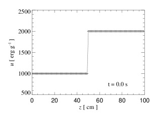
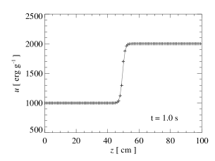
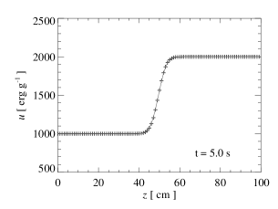
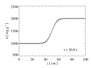
Figure 1: Time evolution of the temperature profile of two slabs of solid material, brought in contact with each other at $t=0$ along the $z=50\,{\rm cm}$ plane, with an initial difference of thermal energy per unit mass of $\Delta u=1000\,{\rm erg\,g^{-1}}$. Crosses mark numerical results, and the solid line is the analytic solution of the heat conduction equation.

To this end, we define a pairwise exchange of heat energy as

$$E_{ij}\equiv\frac{2\mu}{k_{B}}\frac{m_{i}m_{j}\kappa_{ij}}{\rho_{i}\rho_{j}}\left(\frac{A_{j}}{\rho_{j}^{1-\gamma}}-\frac{A_{i}}{\rho_{i}^{1-\gamma}}\right)\frac{{\mn@boldsymbol{x}}_{ij}{\mn@boldsymbol{\nabla}}_{i}W_{ij}}{|{\mn@boldsymbol{x}}_{ij}|^{2}}\text{.}$$ (22)

A simple translation into a finite difference scheme for the time evolution would then be

$$m_{i}u_{i}^{\prime}=m_{i}u_{i}+\Delta t_{i}\sum_{j}E_{ij},$$ (23)

where $u_{i}^{\prime}$ and $u_{i}$ can also be expressed in terms of the corresponding entropy values $A_{i}^{\prime}$ and $A_{i}$. However, for individual and variable timesteps, only a subfraction of particles will be ‘active’ in the current system timestep. These particles have individual timesteps $\Delta t_{i}$, while the ‘inactive’ particles can be formally assigned $\Delta t_{i}=0$ for the step. Equation (23) then clearly does not guarantee detailed energy conservation in each system step.

We recover this property in the following way. We update the energy of particles according to

$$m_{i}u_{i}^{\prime}=m_{i}u_{i}+\frac{1}{2}\sum_{jk}\Delta t_{j}(\delta_{ij}-\delta_{ik})E_{jk}$$ (24)

in each system step. In practice, the double-sum on the right hand side can be simply computed using the usual SPH loop for active particles. Each interacting pair found in the neighbour search for active particle $i$ is simply used to change the thermal energy of particle $i$ by $\Delta t_{i}E_{ij}/2$, and that of the neighbouring particle $j$ by $-\Delta t_{i}E_{ij}/2$ as well. Note that if particle $j$ is active, it carries out a neighbour search itself and will find $i$ itself, so that the total energy change of $i$ due to the presence of $j$ is given by $(\Delta t_{i}+\Delta t_{j})E_{ij}/2$. Energy is conserved by construction in this scheme, independent of the values if individual timesteps of particles. If all particles have equal steps, equation (24) is identical to the form of (23). As before, in our SPH implementation we convert the final thermal energy change to a corresponding entropy change. These entropy changes are applied instantaneously for all particles at the end of one system step, so that even particles that are inactive at the current system step may have their entropy changed by conduction. The resulting low order of the time integration scheme is sufficient for the diffusion equation.

If conduction is so strong that the timescale of conductive redistribution of thermal energy is short compared to relevant dynamical timescales of the gas, the usual hydrodynamic timestep selected by the code based on the Courant-criterion may become too coarse to follow conduction accurately. We therefore introduce an additional timestep criterion in simulations that follow thermal conduction. To this end, we limit the maximum allowed timestep to some prescribed fraction of the conduction time scale, ${A}/{|\dot{A}_{\rm cond}|}$, namely

$$\Delta t_{\rm cond}=\alpha\times\frac{A}{|\dot{A}_{\rm cond}|}\text{,}$$ (25)

where $\alpha$ is a dimensionless accuracy parameter. In our simulations, we typically employed a value of $\alpha=0.25$, which has provided good enough accuracy at a moderate cost of CPU time.

Finally, in order to account for a possible limitation of conduction by saturation, we compute the gradient of the (smoothed) temperature field in the usual SPH fashion, and then use it to compute $l_{T}$ and the saturation-limited conductivity based on equation (8).

3 Illustrative test problems

In this section, we verify our numerical implementation of thermal conduction with a number of simple test problems that have known analytic solutions. We will also investigate the robustness of our formulation with respect to particle disorder, and (initial) noise in the temperature field.

3.1 Conduction in a one-dimensional problem

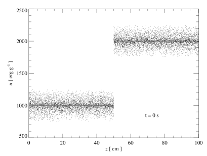
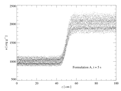
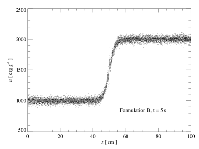
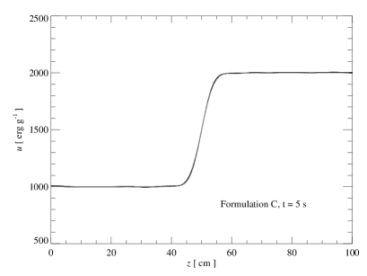
Figure 2: Comparison of the numerical stability of the SPH discretisation scheme when different formulations for the conduction equation (22) are used. The top left panel shows the initial conditions for the simple conduction problem considered in Fig. 1, but perturbed with artificial Gaussian noise in the temperature field. The top right panel shows the evolved state after $5\,{\rm sec}$ when formulation (A) is employed, where the individual particle temperatures are used directly. The lower left panel compares this with formulation (B), where the temperatures on the right hand-side of equation (22) are taken to be kernel interpolants of the temperature field. Finally, the bottom right panel gives the result for formulation (C), which represents a mixed scheme that uses both the individual temperatures of particles, and the smoothed temperature field. This scheme proves to be the most robust against local noise, which is quickly damped away.

We first consider two solid slabs with different initial temperatures, brought into contact with each other at time $t=0$. The slabs were realized as a lattice of SPH particles, with dimensions $100\times 10\times 10$, and an equidistant particle-spacing of $1\ \text{cm}$. To avoid perturbations of the 1D-symmetry, the simulation volume was taken to be periodic along the two short axes, while kept non-periodic along the long axis, allowing us to study surface effects, if present, on the sides of the slabs that are not in contact. Note that the test was carried out with our 3D code. All particle velocities were set to zero initially, and kept at this value to mimic a solid body. The thermal conductivity was set to a value corresponding to $\alpha={\kappa}/{(c_{v}\rho)}=1\ \text{cm}^{2}\,\text{s}^{-1}$ throughout both materials, independent of temperature.

In Figure 1, we compare the time evolution of our numerical results for this test with the analytical solution of the same problem, which is given by

$$u(z,t)=u_{0}+\frac{\Delta u}{2}\,{\rm erf}\left(\frac{z-z_{m}}{\sqrt{4\alpha t}}\right),$$ (26)

where $z_{m}$ gives the position of the initial difference of size $\Delta u$ in thermal energy, and $u_{0}$ is the mean thermal energy. We see that the numerical solution tracks the analytic result very nicely.

We have also repeated the test for a particle configuration corresponding to a ‘glass’ (White, 1996), with equally good results. For a Poisson distribution of particles, we noted however a small reduction in the speed of conduction when a small number of neighbours of 32 is used. Apparently, here the large density fluctuations due to the Poisson process combined with the smallness of the number of neighbours leads to somewhat poor coupling between the particles. This effect goes away for larger numbers of neighbours, as expected. Note however that in practice, due to the pressure forces in a gas, the typical configuration of tracer particles is much more akin to a glass than to a Poisson distribution.

Next, we examine how robust our formulation is with respect to small-scale noise in the temperature field. To this end, we repeat the above test using the glass configuration, but we perturb the initial thermal energies randomly with fluctuations at an rms-level of $\sigma=80\ \text{erg g}^{-1}$. Further, we increase the maximum timestep allowed for particles to $\Delta t=1.0\ \text{s}$.

We discussed previously that we can either use the particle values of the temperatures (or entropy) in the right-hand-side of equation (22), or kernel interpolants thereof. Here we compare the following different choices with each other:

1. Basic formulation: Use particle values $A_{i}$ and $A_{j}$.

2. Smoothed formulation: Use $\overline{A}_{i}$ and $\overline{A}_{j}$.

3. Mixed formulation: Use $A_{i}$ and $\overline{A}_{j}$.

The mixed formulation (C) may at first seem problematic, because its pair-wise antisymmetry is not manifest. However, since we use equation (24) to exchange heat between particles, conservation of thermal energy is ensured also in this case. When all particles have equal timesteps, formulation (C) would correspond to an arithmetic average of (A) and (B).

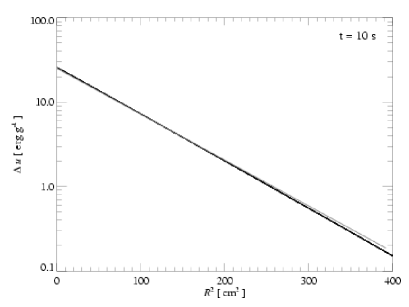
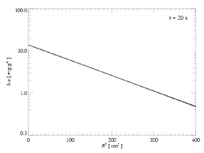
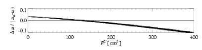
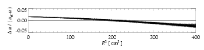
Figure 3: Time evolution of the temperature field in an elementary three-dimensional conduction problem, displayed at two different times. We here consider the spreading of a narrow Gaussian temperature profile, which corresponds to the Green’s function of the conduction problem for constant conductivity. Dots show the specific energies of individual simulation particles, while the solid line marks the analytical result. Relative deviations are shown in the lower panels. The numerical result maintains the Gaussian profile very well at all times. At early times, when the profile is sampled with few particles, a small reduction in the effective speed of conduction is seen, which however becomes increasingly unimportant at later times.

In Figure 2, we compare the result obtained for these three formulations after a simulation time of 5 sec. The artificially perturbed initial conditions are shown in the top left panel. Interestingly, while all three different formulations are able to recover the analytic solution in the mean, they show qualitatively different behaviour with respect to the imprinted noise. When the intrinsic particle values for the temperatures are used (top right panel), very large pair-wise gradients on small scales occur that induce large heat exchanges. As a result, the particles oscillate around the mean, maintaining a certain rms-scatter which does not reduce with time, i.e. an efficient relaxation to the medium temperature does not occur. Note that the absolute size of the scatter is larger in the hot part of the slab. This is a result of the timestep criterion (25), which manages to hedge the rms-noise to something of order $\sim\alpha T$. Reducing the timestep parameter $\alpha$ can thus improve the behaviour, while simultaneously increasing the computational cost significantly. For coarse timestepping (or high conductivities) the integration with this method can easily become unstable.

Formulation (B), which uses the smoothed kernel-interpolated temperature field for both particles in each pair, does significantly better in this respect (bottom left panel). However, the particle temperatures only very slowly approach the local mean value and hence the analytical solution in this case. This is because the smoothing here is quite efficient in eliminating the small-scale noise, meaning that a deviation of an individual particle’s temperature from the local mean is decaying only very slowly.

The mixed formulation (C), shown in the bottom right, obviously shows the best behaviour in this test. It suppresses noise quickly, matches the analytical solution very well, and allows the largest timesteps of all schemes we tested. In this formulation, particles which have a large deviation from the local average temperature try to equalise this difference quickly, while a particle that is already close to the mean is not ‘pulled away’ by neighbours that have large deviations. Apparently, this leads to better behaviour than for schemes (A) and (B), particularly when individual timesteps are used. We hence choose formulation (C) as our default method.

3.2 Conduction in a three-dimensional problem

As a simple test of conduction in an intrinsically three-dimensional problem, we consider the temporal evolution of a point-like thermal energy perturbation. The time evolution of an initial $\delta$-function is given by the three-dimensional Green’s function for the conduction problem,

$$G(x,y,z,t)=\frac{1}{(4\pi\alpha t)^{3/2}}\exp\left(-\frac{x^{2}+y^{2}+z^{2}}{4\alpha t}\right)\text{,}$$ (27)

where $c_{v}=u/T$ is the heat capacity. We again consider a solid material, realized with a glass configuration of $50^{3}$ simulation particles with a mass of $1\,\text{g}$ each and a mean particle spacing of $1\,{\rm cm}$. We choose a conductivity of $\kappa c_{v}=1\,\text{cm}^{2}\,\text{s}^{-1}$, as before. We give the material a specific energy per unit mass of $u_{0}=1000\,\text{erg}\ \text{g}^{-1}$, and add a perturbation of $10000.0\ \text{erg}\ \text{cm}^{3}\,\text{g}^{-1}\times G(x,y,z,t_{0}=10\ \text{sec})$. These initial conditions correspond to a $\delta$-function perturbation that has already evolved for a brief period; this should largely eliminate timing offsets that would arise in the later evolution if we let the intrinsic SPH smoothing wash out a true initial $\delta$-function.

Figure 3 shows the specific energy profile after evolving the conduction problem for an additional 10 or 20 seconds, respectively. In the two bottom panels, we show the relative deviation from the analytic solution. Given that quite coarse timestepping was used for this problem (about $\sim 32$ timesteps for 20 sec), the match between the theoretical and numerical solutions is quite good. Even at a radial distance of $20\,\text{cm}$, where the Gaussian profile has dropped to less than one hundredth of its central amplitude, relative deviations are at around 10 percent for $t=20\ \text{sec}$ and below 3 percent at $t=30\ \text{sec}$. Note however that at all times the numerical solution maintains a nice Gaussian shape so that the deviations can be interpreted as a small modification in the effective conductivity. We then see that at late times, when the temperature gradients are resolved by more particles, the SPH estimate of the conductivity becomes ever more accurate.

4 Spherical models for clusters of galaxies

Observed temperature profiles of clusters of galaxies are often characterised by a central decline of temperature, while otherwise appearing fairly isothermal over the measurable radial range. Provided the conductivity is non-negligible, there should hence be a conductive heat flux into the inner parts, which would then counteract central cooling losses. Motivated by this observation, Zakamska & Narayan (2003) (ZN henceforth) have constructed simple analytic models for the structure of clusters, invoking as a key assumption a local equilibrium between conduction and cooling. Combined with the assumption of hydrostatic equilibrium and spherical symmetry, they were able to quite successfully reproduce the temperature profiles of a number of observed clusters.

We here use the model of ZN as a test-bed to check the validity of our conduction modelling in a realistic cosmological situation. In addition, the question for how long the ZN solution can be maintained is of immediate interest, and we address this with our simulations of spherical clusters as well.

For definiteness, we briefly summarise the method of ZN for constructing a cluster equilibrium model. The cluster is assumed to be spherically symmetric, with the gas of density $\rho(r)$ and pressure $P(r)$ being in hydrostatic equilibrium, i.e.

$$\frac{1}{\rho}\frac{\text{d}P}{\text{d}r}=-\frac{\text{d}\Phi}{\text{d}r},$$ (28)

where the gravitational potential $\Phi$ is given by

$$\frac{1}{r^{2}}\frac{\text{d}}{\text{d}r}\left(r^{2}\frac{\text{d}\Phi}{\text{d}r}\right)=4\pi G\left(\rho_{\rm DM}+\rho\right)\text{.}$$ (29)

The dark matter density $\rho_{\rm DM}(r)$ is described by a standard NFW (Navarro, Frenk & White, 1996) halo, optionally modified by ZN with the introduction of a small softened dark matter core. The structure of the dark halo can then be fully specified by the virial radius $r_{\rm 200}$, defined as the radius enclosing a mean overdensity of 200 with respect to the critical density, and a scale length $r_{s}$.

The radial heat flux $F$ due to electron conduction is given by

$$F=-\kappa\frac{\text{d}T}{\text{d}r},$$ (30)

where the conductivity $\kappa$ is taken to be a constant fraction of the Spitzer value. In order to balance local cooling losses, we require

$$\frac{1}{r^{2}}\frac{\text{d}}{\text{d}r}\left(r^{2}F\right)=-j,$$ (31)

where $j$ is describing the local gas cooling rate. If cooling is dominated by thermal bremsstrahlung, $j$ can be approximated as

$$j=2.1\times 10^{-27}n_{e}^{2}\,T^{1/2}\,\text{ergs cm}^{-3}\text{s}^{-1}.$$ (32)

The electron number density $n_{e}$ herein correlates with the gas density $\rho$ and depends on the hydrogen mass fraction $X$ we assume for the primordial matter. With a proton mass of $m_{p}$, it equals $n_{e}=\rho(X+1)/(2m_{p})$. Following ZN, we use this simplification in setting up our cluster models.

Equations (28) to (32) form a system of differential equations that can be integrated from inside out once appropriate boundary conditions are specified. We adopt the values for central gas density and temperature, total dark matter mass, and scale radius determined by ZN for the cluster A2390 such that the resulting temperature profile matches the observed one well in the range $0\leq r\leq R_{\rm out}$, where $R_{\rm out}$ was taken to be $2\,r_{s}$.

Figure 4: Local cooling (solid line) and conductive heating rates (dotted line) as a function of radius in our model for the cluster A2390, after a time of $t=0.15\,\,\text{Gyr}$. It is seen that both energy transfer rates cancel each other with reasonable accuracy.

Integrating the system of equations out to $R_{\rm out}$, we obtain a result that very well matches that reported by ZN. However, we also need to specify the structure of the cluster in its outer parts in order to be able to simulate it as an isolated system. ZN simply assumed this part to be isothermal at the temperature $T_{\rm out}=T(R_{\rm out})$, thereby implicitly assuming that the equilibrium condition between cooling and conduction invoked for the inner parts is not valid any more. It is a bit unclear why such a sudden transition should occur, but the alternative assumption, that equation (31) holds out to the virial radius, clearly leads to an unrealistic global temperature profile. In this case, the temperature would have to monotonically increase out to the outermost radius. Also, since the cumulative radiative losses out to a radius $r$ have to be balanced by a conductive heat flux of equal magnitude at that radius, the heat flux also monotonically increases, such that all the energy radiated by the cluster would have to be supplied to the cluster at the virial radius.

We nevertheless examined both approaches, i.e. we construct cluster models where we solve equations (28)-(32) for the whole cluster out to a radius of $r_{\rm 200}$, and secondly, we construct initial conditions where we follow ZN by truncating the solution at $2\,r_{\rm s}$, continuing into the outer parts with an isothermal solution that is obtained by dropping equations (30) and (31). Since conduction may still be important at radii somewhat larger than $2\,r_{s}$, these two models may hence be viewed as bracketing the expected real behaviour of the cluster in a model where cooling is balanced by conduction.

Figure 5: Temperature profile (left) and cumulative mass profile (right) of our model for the cluster A2390, after a simulated time of $0.6\,\,\text{Gyr}$. We compare simulations with (triangles) and without (diamonds) thermal conduction using a conductivity of $0.3\,\kappa_{\rm sp}$. It is seen that without conduction, the inner regions of the cluster cool down significantly, causing mass to sink towards the centre as central pressure support is partially lost. If thermal conduction is included, the central cooling losses are offset by conductive heating from outer regions, preventing any significant change of the baryonic mass profile. In fact, in this case we even observe a slow secular evolution towards higher temperature in the inner parts.

For the plasma conductivity, we assumed a value of $0.3\,\kappa_{\rm sp}$, as proposed by ZN in their best-fit solution for A2390. Note that this value implies that a certain degree of suppression of conduction by magnetic fields is present, but that this effect is (perhaps optimistically) weak, corresponding to what is expected for chaotically tangled magnetic fields (Narayan & Medvedev, 2001).

Having obtained a solution for the static cluster model, we realized it as 3D initial conditions for GADGET. We used $2\times 10^{5}$ gas particles with a total baryonic mass of around $8.6\times 10^{14}\ \text{M}_{\odot}$. For simplicity, we described the NFW dark matter halo of mass $2.4\times 10^{15}\,{\rm M_{\odot}}$ as a static potential. We then simulated the evolution of the gas subject to self-gravity (with a gravitational softening length of $3\,\text{kpc}$), radiative cooling, and thermal conduction, but without allowing for star formation and associated feedback processes.

By construction, we expect that thermal conduction will be able to offset radiative cooling for these initial conditions, at least for some time. This can be verified in Figure 4, where we plot the local cooling rate and conductive heating rate as a function of radius. Indeed, at time $0.15\,{\rm Gyr}$, after a brief initial relaxation period, the two energy transfer rates exhibit the same magnitude and cancel each other with good accuracy. This represents a nice validation of our numerical implementation of thermal conduction with the temperature-dependent Spitzer-rate.

As the simulation continues, we see that the core temperature of the cluster slowly drifts to somewhat higher temperature. A secular evolution of some kind is probably unavoidable, since the balance between cooling and conductive heating cannot be perfectly static. The cluster of course still loses all the energy it radiates, which eventually must give rise to a slow quasi-static inflow of gas, and a corresponding change of the inner structure of the cluster. Because of the different temperature dependences of cooling and conductive heating, it is also not clear that the balance between cooling and conductive heating represents a stable dynamical state. While a stability analysis by ZN and Kim & Narayan (2003) suggests that thermal instability is sufficiently suppressed in models with conduction, Soker (2003) argues that local perturbations in the cooling flow region will grow to the non-linear regime rather quickly and that a steady solution with a constant heat conduction may therefore not exist.

In any case, it is clear that the inclusion of conduction strongly reduces central mass drop out due to cooling. This is demonstrated explicitly in Figure 5, where we show the temperature and cumulative baryonic mass profiles of the cluster after a time of $0.6\,{\rm Gyr}$. We compare these profiles also to an identical simulation where conduction was not included. Unlike the conduction run, this cooling-only simulation shows a very substantial modification of its temperature profile in the inner parts, where the core region inside $\sim 0.1\,{\rm Mpc}$ becomes much colder than the initial state. We can also see that the cooling-only simulation has seen substantial baryonic inflow as a result of central mass drop-out. Within $0.6\,{\rm Gyr}$, the baryonic mass enclosed in a sphere with radius $50\,{\rm kpc}$ has increased by 86 percent in this simulation, clearly forming a cooling flow. This contrasts strongly with the run that includes conduction, where beyond a cental distance of $\sim 0.02\,{\rm Mpc}$, there is no significant difference in the cumulative mass profile between $t=0$ and $t=0.6\,{\rm Gyr}$.

We also checked that runs with a reduced conductivity show a likewise reduced effect, suppressing the core cooling and matter inflow to a lesser extent than with our default model with $0.3\,\kappa_{\rm sp}$.

Finally, we note that the results discussed here are quite insensitive to whether we set-up the initial conditions with an isothermal outer part, or whether we continue the equilibrium solution to the virial radius. There is only a small difference in the long term evolution of the solution.

The model presented here helps us to verify the robustness of our conduction implementation when a temperature dependent conductivity is used, but it does not account for the time dependence of conduction expected in the cosmological context. The static, spherically symmetric construction does not reflect the hierarchical growth of clusters that is a central element of currently favoured cosmologies. To be able to make reliable statements about the effects of thermal conduction on galaxy clusters, one therefore has to trace their evolution from high redshift to the present, which is best done in full cosmological simulations. Here, the hierarchical growth of clusters implies that the conductivity is becoming low early on, when the ICM temperature is low, and becomes only large at late times when the cluster forms.

5 Cosmological Cluster Simulations

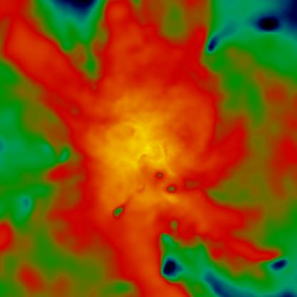
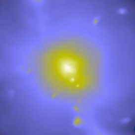
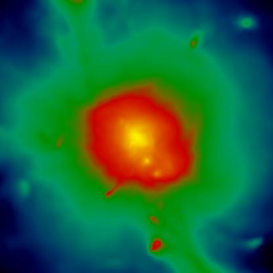
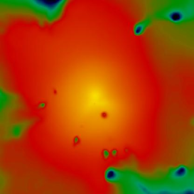
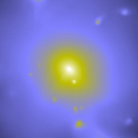
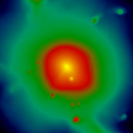
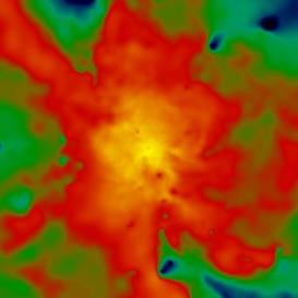
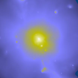
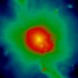
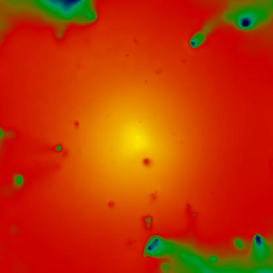
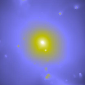
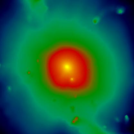
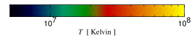
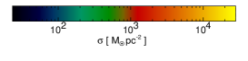
Figure 6: Projections of mass-weighted temperature (left column), X-ray emissivity (middle column), and gas mass density (right column) for our cluster simulations at $z=0.13$. From the top to the bottom row, we show the same cluster but simulated with different physics: Adiabatic gasdynamics only, adiabatic plus thermal conduction, radiative cooling and star formation, and finally, cooling, star formation and conduction. Each panel displays the gas contained in a box of side-length $8.6\,{\rm Mpc}$ centred on the cluster. Full Spitzer conductivity was assumed.

Figure 7: Cumulative baryonic mass profile (top), temperature profile (middle) and X-ray emissivity profile (bottom) of the simulated cluster at $z=0.13$. In each panel, we compare the same cluster simulation run with different physical models for the gas: Adiabatic gasdynamics only, adiabatic plus thermal conduction, radiative cooling and star formation without conduction, and finally, cooling, star formation and conduction. For the models including conduction, full Spitzer conductivity was assumed. Note that the X-ray emissivity is plotted such that the area under the curve is proportional to the total bolometric X-ray luminosity.

In this section, we apply our new numerical scheme for the treatment of thermal conduction in fully self-consistent cosmological simulations of cluster formation. We will in particular compare the results of simulations with and without conduction, both for runs that follow only adiabatic gas-dynamics, and runs that also include radiative cooling of gas. While it is beyond the scope of this work to present a comprehensive analysis of the effects of conduction in cosmological simulations, we here want to investigate a set of small fiducial runs in order to further validate the stability of our method for real-world applications, and secondly, to give a first flavour of the expected effects of conduction in simulated clusters. A more detailed analysis of cosmological implications of conduction is presented in a companion paper (Dolag et al., 2004).

We focus on a single cluster, extracted from the ‘GIF’ simulation (Kauffmann et al., 1999) of the $\Lambda$CDM model, and resimulated using the “zoomed initial conditions” technique (Tormen et al., 1997). To this end, the particles that make up the cluster at the present time are traced back to their original coordinates in the initial conditions. The Lagrangian region of the cluster identified in this way is then resampled with particles of smaller mass, and additional small-scale perturbations from the CDM power spectrum are added appropriately. Far away from the cluster, the resolution is progressively degraded by using particles of ever larger mass.

The cluster we selected has a virial mass of $1.1\times 10^{15}\,{\rm M}_{\odot}$. It is the same cluster considered in the high-resolution study of Springel et al. (2001a), with our mass resolution corresponding to their S1 simulation, except that we split each of the $\sim 450000$ high resolution dark matter particles into a gas and a dark matter particle (assuming $\Omega_{b}=0.04$), yielding a gas mass resolution of $8.4\times 10^{9}\,{\rm M_{\odot}}$. The boundary region was sampled with an additional 3 million dark matter particles. We then evolved the cluster forward in time from a starting redshift $z=30$ to the present, $z=0$, using a comoving gravitational softening length of $20\,{\rm kpc}$.

We consider 4 different simulations of the cluster, each with different physical models for the gas: (1) Adiabatic gasdynamics only, (2) adiabatic gas and conduction, (3) radiative cooling and star formation without conduction, and finally, (4) radiative cooling, star formation and conduction. The simulations with cooling and star formation use the sub-resolution model of Springel & Hernquist (2003) for the multi-phase structure of the ISM (without including the optional feedback by galactic winds offered by the model). In the two runs with conduction, we adopt the full Spitzer rate for the conductivity. While this value is unrealistically large for magnetised clusters, it serves our purpose here in highlighting the effects of conduction, given also that our cluster is not particularly hot, so that effects of conductivity can be expected to be weaker than in very rich clusters.

In Figure 6, we show projections of the mass-weighted temperature, X-ray emissivity, and gas mass density for all four simulations. Each panel displays the gas contained in a box of side-length $8.6\,{\rm Mpc}$ centred on the cluster. Comparing the simulations with and without conduction, it is nicely seen how conduction tends to wipe out small-scale temperature fluctuations. It is also seen that the outer parts of the cluster become hotter when conduction is included.

These trends are also borne out quantitatively when studying radial profiles of cluster properties in more detail. In Figure 7, we compare the cumulative baryonic mass profile, the temperature profile, and the radial profile of X-ray emission for all four simulations. Note that the innermost bins, for $R<30\,{\rm kpc}$, may be affected by numerical resolution effects. Interestingly, the temperature profiles of the runs with conduction are close to being perfectly isothermal in the inner parts of the cluster. While this does not represent a large change for the adiabatic simulation, which is close to isothermal anyway, the simulation with radiative cooling is changed significantly. Without conduction, the radiative run actually shows a pronounced rise in the temperature profile in the range of $100-200\,{\rm kpc}$, as a result of compressional heating when gas flows in to replace gas that is cooling out of the ICM in a cooling flow. Only in the innermost regions, where cooling becomes rapid, we see a distinct drop of the temperature. Interestingly, conduction eliminates this feature in the temperature profile, by transporting the corresponding heat energy from the maximum both to parts of the cluster further out and to the innermost parts. The latter effect is probably small, however, because a smooth decline in the temperature profile in the inner parts of the cluster, as present in the ZN model, does not appear in the simulation. As a consequence, a strong conductive heat flow from outside to inside cannot develop.

Conduction may also induce changes in the X-ray emission of the clusters, which we show in the bottom panel of Figure 7. Interestingly, the inclusion of conduction in the adiabatic simulation has a negligible effect on the X-ray luminosity. This is because in contrast to previous suggestions (Loeb, 2002), the cluster does not lose a significant fraction of its thermal energy content to the outside intergalactic medium, and the changes in the relevant part of the gas and temperature profile are rather modest. We do note however that the redistribution of thermal energy within the cluster leads to a substantial increase of the temperature of the outer parts of the cluster.

For the simulations with cooling, the changes of the X-ray properties are more significant. Interestingly, we find that allowing for thermal conduction leads to a net increase of the bolometric luminosity of our simulated cluster. The panel with the cumulative baryon mass profile reveals that conduction is also ineffective in significantly suppressing the condensation of mass in the core regions of the cluster. In fact, it may even lead to the opposite effect. We think this behaviour simply occurs because a temperature profile with a smooth decline towards the centre, which would allow the conductive heating of this part of the cluster, is not forming in the simulation. Instead, the conductive heat flux is pointing primarily from the inside to the outside, which may then be viewed as an additional “cooling” process for the inner cluster regions.

It is interesting to note that in spite of the structural effects that thermal conduction has on the ICM of the cluster, it does not affect its star formation history significantly. In the two simulations that include cooling and star formation, the stellar component of the mass profile (Figure 7) does not show any sizeable difference between the run including thermal conduction and the one without it. This does not come as surprise as $90\%$ of the stellar content of the cluster has formed before a redshift of $z=0.85$. At these early times, the temperature of the gas in the protocluster was much lower, such that conduction was unimportant. In fact, for that reason, the stellar mass profiles for both simulation runs coincide.

In summary, our initial results for this cluster suggest that conduction can be important for the ICM, provided the effective conductivity is a sizable fraction of the Spitzer value. However, the interplay between radiative cooling and conduction is clearly complex, and it is presently unclear whether temperature profiles like those observed can arise in self-consistent cosmological simulations. We caution that one should not infer too much from the single object we examined here. A much larger set of cluster simulations will be required to understand this topic better.

6 Conclusions

Hot plasmas like those found in clusters of galaxies are efficiently conducting heat, unless electron thermal conduction is heavily suppressed by magnetic fields. Provided the latter is not the case, heat conduction should therefore be included in hydrodynamical cosmological simulations, given, in particular, that conduction could play a decisive role in moderating cooling flows in clusters of galaxies. Such simulations are then an ideal tool to make reliable predictions of the complex interplay between the nonlinear processes of cooling and conduction during structure formation.

In this paper, we have presented a detailed numerical methodology for the treatment of conduction in cosmological SPH simulations. By construction, our method manifestly conserves thermal energy, and we have formulated it such that it is robust against the presence of small-scale temperature noise. We have implemented this method in a modern parallel code, capable of carrying out large, high-resolution cosmological simulations.

Using various test problems, we have demonstrated the accuracy and robustness of our numerical scheme for conduction. We then applied our code to a first set of cosmological cluster formation simulations, comparing in particular simulations with and without conduction. While these results are preliminary, they already hint that the phenomenology of the coupled dynamics of radiative cooling and conduction is complex, and may give rise to results that were perhaps not anticipated by earlier analytic modelling of static cluster configurations.

For example, we found that conduction does not necessarily reduce a central cooling flow in our simulations; the required smoothly declining temperature profile in the inner cluster regions does not readily form in our cosmological simulations. Instead, the profiles we find are either flat, or have a tendency to slightly rise towards the centre, akin to what is seen in the cooling-only simulations. In this situation, conduction may in fact lead to additional cooling in certain situations, by either transporting thermal energy to the outer parts, or by modifying the temperature and density structure in the relevant parts of the cluster such that cooling is enhanced. This can then manifest itself in an increase of the bolometric X-ray luminosity at certain times, which is actually the case for our model cluster at $z=0$. Interestingly, we do not find that our cluster loses a significant fraction of its thermal heat content by conducting it to the external intergalactic medium.

In a companion paper (Dolag et al., 2004), we analyse a larger set of cosmological cluster simulations, computed with much higher resolution and with more realistic sub-Spitzer conductivities. This set of cluster allows us to investigate, e.g., conduction effects as a function of cluster temperature and the influence of conduction on cluster scaling relations. While our first results of this work suggest that conduction by itself may not resolve the cooling-flow puzzle, it also shows that conduction has a very strong influence on the thermodynamic state of rich clusters if the effective conductivity is a small fraction of the Spitzer value or more. In future work, it will hence be very interesting and important to understand the rich phenomenology of conduction in clusters in more detail.

References

- Allen et al. (2001) Allen S. W., Schmidt R. W., Fabian A. C., 2001, MNRAS, 328, L37
- Borgani et al. (2003) Borgani S., Murante G., Springel V., et al., 2003, MNRAS, in press
- Bower et al. (2001) Bower R. G., Benson A. J., Lacey C. G., Baugh C. M., Cole S., Frenk C. S., 2001, MNRAS, 325, 497
- Brookshaw (1985) Brookshaw L., 1985, Proceedings of the Astronomical Society of Australia, 6, 207
- Brüggen (2003) Brüggen M., 2003, ApJ, 593, 700
- Carilli & Taylor (2002) Carilli C. L., Taylor G. B., 2002, ARA&A, 40, 319
- Chandran & Cowley (1998) Chandran B. D. G., Cowley S. C., 1998, Physical Review Letters, 80, 3077
- Churazov et al. (2001) Churazov E., Brüggen M., Kaiser C. R., Böhringer H., Forman W., 2001, ApJ, 554, 261
- Cleary & Monaghan (1999) Cleary P. W., Monaghan J. J., 1999, Journal of Computational Physics, 148, 227
- Cowie & McKee (1977) Cowie L. L., McKee C. F., 1977, ApJ, 211, 135
- David et al. (2001) David L. P., Nulsen P. E. J., McNamara B. R., et al., 2001, ApJ, 557, 546
- Dolag et al. (2004) Dolag K., Jubelgas M., Springel V., Borgani S., Rasia E., 2004, ApJ, submitted, astro-ph/0401470
- Enßlin & Heinz (2001) Enßlin T. A., Heinz S., 2001, A&A, 384, 27
- Ettori & Fabian (2000) Ettori S., Fabian A. C., 2000, MNRAS, 317, L57
- Ettori et al. (2002) Ettori S., Fabian A. C., Allen S. W., Johnstone R. M., 2002, MNRAS, 331, 635
- Fabian (1994) Fabian A. C., 1994, ARA&A, 32, 277
- Fabian et al. (2002) Fabian A. C., Voigt L. M., Morris R. G., 2002, MNRAS, 335, L71
- Frenk et al. (1999) Frenk C. S., White S. D. M., Bode P., et al., 1999, ApJ, 525, 554
- Fujita et al. (2003) Fujita Y., Suzuki T. K., Wada K., 2003, ApJ, in press
- Johnstone et al. (2002) Johnstone R. M., Allen S. W., Fabian A. C., Sanders J. S., 2002, MNRAS, 336, 299
- Kauffmann et al. (1999) Kauffmann G., Colberg J. M., Diaferio A., White S. D. M., 1999, MNRAS, 303, 188
- Kim & Narayan (2003) Kim W., Narayan R., 2003, ApJ, 596, 889
- Lewis et al. (2000) Lewis G. F., Babul A., Katz N., Quinn T., Hernquist L., Weinberg D. H., 2000, ApJ, 536, 623
- Lloyd-Davies et al. (2000) Lloyd-Davies E. J., Ponman T. J., Cannon D. B., 2000, MNRAS, 315, 689
- Loeb (2002) Loeb A., 2002, New Astronomy, 7, 279
- Loewenstein (2000) Loewenstein M., 2000, ApJ, 532, 17
- Lucy (1977) Lucy L. B., 1977, AJ, 82, 1013
- Malyshkin & Kulsrud (2001) Malyshkin L., Kulsrud R., 2001, ApJ, 549, 402
- Markevitch et al. (2000) Markevitch M., Ponman T. J., Nulsen P. E. J., et al., 2000, ApJ, 541, 542
- Medvedev et al. (2003) Medvedev M. V., Melott A. L., Miller C., Horner D., 2003, preprint, astro-ph/0303310
- Menci & Cavaliere (2000) Menci N., Cavaliere A., 2000, Bulletin of the American Astronomical Society, 32, 1200
- Metzler & Evrard (1994) Metzler C. A., Evrard A. E., 1994, ApJ, 437, 564
- Monaghan (1992) Monaghan J. J., 1992, ARA&A, 30, 543
- Monaghan & Lattanzio (1985) Monaghan J. J., Lattanzio J. C., 1985, A&A, 149, 135
- Narayan & Medvedev (2001) Narayan R., Medvedev M. V., 2001, ApJL, 562, L129
- Navarro et al. (1996) Navarro J. F., Frenk C. S., White S. D. M., 1996, ApJ, 462, 563
- Ponman et al. (1999) Ponman T. J., Cannon D. B., Navarro J. F., 1999, Nature, 397, 135
- Sarazin (1988) Sarazin C. L., 1988, X-ray emission from clusters of galaxies, Cambridge Astrophysics Series, Cambridge: Cambridge University Press, 1988
- Soker (2003) Soker N., 2003, MNRAS, 342, 463
- Spitzer (1962) Spitzer L., 1962, Physics of Fully Ionized Gases, Physics of Fully Ionized Gases, New York: Interscience (2nd edition), 1962
- Springel & Hernquist (2002) Springel V., Hernquist L., 2002, MNRAS, 333, 649
- Springel & Hernquist (2003) Springel V., Hernquist L., 2003, MNRAS, 339, 289
- Springel et al. (2001a) Springel V., White S. D. M., Tormen B., Kauffmann G., 2001a, MNRAS, 328, 726
- Springel et al. (2001b) Springel V., Yoshida N., White S. D. M., 2001b, New Astronomy, 6, 79
- Tormen et al. (1997) Tormen G., Bouchet F. R., White S. D. M., 1997, MNRAS, 286, 865
- Tornatore et al. (2003) Tornatore L., Borgani S., Springel V., Matteucci F., Menci N., Murante G., 2003, MNRAS, 342, 1025
- Vikhlinin et al. (2001) Vikhlinin A., Markevitch M., Murray S. S., 2001, ApJ, 551, 160
- Vogt & Enßlin (2003) Vogt C., Enßlin T. A., 2003, A&A, in press
- Voigt & Fabian (2003) Voigt L. M., Fabian A. C., 2003, MNRAS, preprint, astro-ph/0308352
- Voigt et al. (2002) Voigt L. M., Schmidt R. W., Fabian A. C., Allen S. W., Johnstone R. M., 2002, MNRAS, 335, L7
- Voit et al. (2002) Voit G. M., Bryan G. L., Balogh M. L., Bower R. G., 2002, ApJ, 576, 601
- White (1996) White S. D. M., 1996, in Cosmology and Large-Scale Structure, edited by R. Schaeffer, J. Silk, M. Spiro, J. Zinn-Justin, 395, Elsevier, Dordrecht
- Wu et al. (1999) Wu K. K. S., Fabian A. C., Nulsen P. E. J., 1999, ArXiv Astrophysics e-prints
- Wu & Xue (2002) Wu X., Xue Y., 2002, ApJL, 572, L19
- Zakamska & Narayan (2003) Zakamska N. L., Narayan R., 2003, ApJ, 582, 162