OPTICAL SELECTION OF GALAXIES AT REDSHIFTS $1<Z<3$

Abstract

Few galaxies have been found between the redshift ranges $z\lower 2.15277pt\hbox{$\;\buildrel<\over{\sim}\;$}1$ probed by magnitude-limited surveys and $z\lower 2.15277pt\hbox{$\;\buildrel>\over{\sim}\;$}3$ probed by Lyman-break surveys. Comparison of galaxy samples at lower and higher redshift suggests that large numbers of stars were born and the Hubble sequence began to take shape at the intermediate redshifts $1<z<3$, but observational challenges have prevented us from observing the process in much detail. We present simple and efficient strategies that can be used to find large numbers of galaxies throughout this important but unexplored redshift range. All the strategies are based on selecting galaxies for spectroscopy on the basis of their colors in ground-based images taken through a small number of optical filters: $G{\cal R}i$ for redshifts $0.85<z<1.15$, $G{\cal R}z$ for $1<z<1.5$, and $U_{n}G{\cal R}$ for $1.4<z<2.1$ and $1.9<z<2.7$. The performance of our strategies is quantified empirically through spectroscopy of more than 2000 galaxies at $1<z<3.5$. We estimate that more than half of the UV-luminosity density at $1<z<3$ is produced by galaxies that satisfy our color-selection criteria. Our methodology is described in detail, allowing readers to devise analogous selection criteria for other optical filter systems.

1. INTRODUCTION

As the photons from the microwave background stream towards earth they are gradually joined by other photons, first by those produced in the occasional recombinations of the intergalactic medium, later by those cast off from cooling $H_{2}$ molecules, later still, after hundreds of millions of years, by increasing numbers from quasars and galaxies, by bremsstrahlung from the hot gas in galaxy groups and clusters, and finally, shortly before impact, by photons emitted by the Milky Way’s own gas and stars and dust. All reach the earth together. They provide a record of the history of the universe throughout its evolution, but it is a confused record. Two photons that simultaneously pierce the same pixel of a detector may have been emitted billions of years apart by regions of the universe that were in vastly different stages of evolution. One of the challenges in observational cosmology is to separate the layers of history that we on earth receive superposed.

This paper is concerned with a small part of the challenge: locating galaxies at redshifts $1\lower 2.15277pt\hbox{$\;\buildrel<\over{\sim}\;$}z\lower 2.15277pt\hbox{$\;\buildrel<\over{\sim}\;$}3$ among the countless objects that speckle the night sky. The redshift range is interesting for a number of reasons. During the $\sim 4$ billion years that elapsed between redshifts 3 and 1, the comoving density of star formation was near its peak, the Hubble sequence of galaxies may have been established, and a large fraction of the stars in the universe were born (Dickinson et al. 2003, Rudnick et al. 2003). Observing star-formation at these redshifts will likely play an important role in our attempts to understand galaxy formation.

Identifying galaxies at $1<z<3$ would be easy if observing time were infinite. One could simply obtain a spectrum of every object in a deep image and discard those at lower or higher redshift. In practice telescope time is limited and one would like to spend as much of it as possible studying objects of interest—not finding them. Our aim is to present simple strategies that allow observers to locate star-forming galaxies at $1<z<3$ with only a minimal loss of telescope time to deep imaging or spectroscopy of objects at the wrong redshifts.

We shall assume throughout that the goal is to identify star-forming galaxies that lie inside a narrow range of redshifts within the wider span $1<z<3$. Concentrating on a narrow range has obvious observational advantages; galaxies at similar redshifts have similar spectral features that lie at similar observed wavelengths, and consequently the spectrograph can be chosen and configured in a way that is optimized for every object on a multislit mask. It is also necessary for many scientific programs. One might want to discover where galaxies lie relative to the intergalactic gas that produces absorption lines in the spectra of a QSO at $z\sim 2.5$, for example, or to create a large and homogeneous sample of galaxies at a single epoch in the past that can then be compared to existing samples of galaxies in the local universe. Projects with wildly different goals may benefit less from the strategies we advocate. Standard magnitude-limited spectroscopy or photometric redshifts might be preferable if (for example) one wanted to create a sample that contained all galaxy types at all redshifts.

Our approach exploits the fact that the wavelength-dependent cross-sections of various common atoms and ions give distinctive colors to galaxies at different redshifts. It has been recognized for decades that measuring a galaxy’s brightness through a range of broad-band filters should therefore provide some indication of its redshift (e.g., Baum 1962; Koo 1985; Loh & Spillar 1986). Recent work suggests that a redshift accuracy of $\sigma_{z}\lower 2.15277pt\hbox{$\;\buildrel<\over{\sim}\;$}0.1$ can be achieved for galaxies at $0\lower 2.15277pt\hbox{$\;\buildrel<\over{\sim}\;$}z\lower 2.15277pt\hbox{$\;\buildrel<\over{\sim}\;$}6$ given extravagantly precise photometry through 7 filters that span the wavelength range $0.3\lower 2.15277pt\hbox{$\;\buildrel<\over{\sim}\;$}\lambda\lower 2.15277pt\hbox{$\;\buildrel<\over{\sim}\;$}2.2\mu$m (e.g., Hogg et al. 1998; Budavári et al. 2000; Fernández-Soto et al. 2001; Rowan-Robinson 2003). An accuracy $\sigma_{z}\lower 2.15277pt\hbox{$\;\buildrel<\over{\sim}\;$}0.1$ is clearly sufficient for finding galaxies at $1<z<3$, but obtaining the necessary deep images through numerous filters consumes enormous amounts of telescope time that could be more profitably devoted to galaxy spectroscopy. We were led to seek specialized color-selection techniques that could identify galaxies at $1<z<3$ even in comparatively noisy images taken through a small number of optical filters.

Such techniques can succeed only if they take advantage of strong and obvious features in galaxies’ spectra. No feature is stronger than the Lyman break at 912Å produced by the photo-electric opacity of hydrogen in its ground state. Meier (1976) argued that the strength of this break would allow high-redshift galaxies to be identified in images taken through just three filters, a claim that Steidel et al. (1996; 1999) have since confirmed. Although the Lyman break itself is not visible from the ground at $z\lower 2.15277pt\hbox{$\;\buildrel<\over{\sim}\;$}3$, other weaker features are, and the success of two-color selection at $z>3$ inspired us try to develop similar two-color optical selection strategies for $1<z<3$. Figure 1 shows some of the spectral features that we had to work with. Most obvious, after the Lyman-break, is the Balmer-break at 3700Å. The strength of the Balmer-break can be estimated from the model galaxy spectra described in § 2 or from the galaxy observations described in § 3. § 4 explains how it can be used to find galaxies at $1\lower 2.15277pt\hbox{$\;\buildrel<\over{\sim}\;$}z\lower 2.15277pt\hbox{$\;\buildrel<\over{\sim}\;$}1.5$. Franx et al. (2003) and Davis et al. (2003) have also used this feature to find distant galaxies. At $1.5\lower 2.15277pt\hbox{$\;\buildrel<\over{\sim}\;$}z\lower 2.15277pt\hbox{$\;\buildrel<\over{\sim}\;$}2.5$ no strong breaks are present in the optical spectra of galaxies, but the lack of spectral breaks is itself a distinguishing characteristic of galaxies at these redshifts. §§ 5, 6, and 7 explain. Our results are summarized and discussed in § 8. Together with the Lyman-break technique, the selection techniques presented here allow the efficient creation of large samples of star-forming galaxies throughout the redshift range $1\lower 2.15277pt\hbox{$\;\buildrel<\over{\sim}\;$}z\lower 2.15277pt\hbox{$\;\buildrel<\over{\sim}\;$}5$.

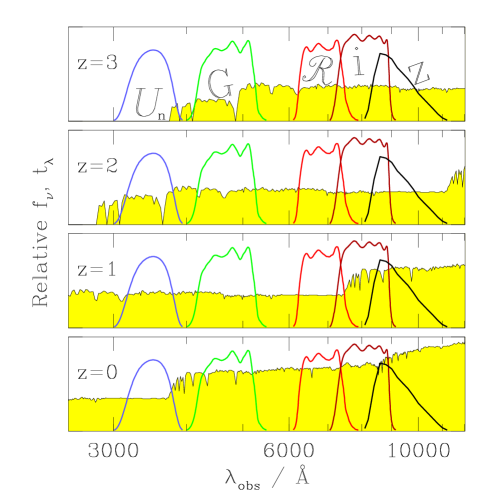
Figure 1.— $U_{n}G{\cal R}iz$ colors of galaxies at redshifts $0<z<3$. Shaded curves show the spectrum of a model star-forming galaxy (type Im from § 2) at various redshifts. Unshaded curves show the transmission curves of the filters used in this paper.

2. MODEL GALAXY SPECTRA

Our development of selection strategies began with theoretical models of galaxy spectra. At redshifts $z\lower 2.15277pt\hbox{$\;\buildrel<\over{\sim}\;$}3$ a galaxy’s optical broad-band colors are determined by the mixture of stellar types it contains. This is in turn largely determined by a galaxy’s star-formation history. Galaxies that formed most of their stars recently have spectra dominated by bright and hot massive stars, while galaxies that formed most of their stars in the distant past will have spectra dominated by fainter, cooler, but longer-lived low-mass stars. We considered five model galaxy spectra that were intended to span the range of possible star-formation histories. Each model spectrum was calculated with the code of Bruzual & Charlot (1996, private communication) and assumed that the galaxy’s star-formation rate as a function of time, $S(t)$, was a decaying exponential: $S(t)\propto\exp(-t/\tau)$. The adopted values of $\tau$ and assumed time-lapse since the onset of star formation for our five models are listed in Table 1. Bruzual & Charlot (1993) show that star-formation histories with these parameters reproduce the observed spectra of different galaxy types in the local universe. Because a wide range of star-formation histories can result in nearly identical model spectra, we were not concerned that some of our adopted model parameters are physically impossible at high redshift due to the young age of the universe. Parameter combinations that are more plausible can produce similar spectra, and in any case our aim was only to have model spectra that roughly spanned the range of conceivability. Subsequent empirical refinements of our selection criteria would compensate for any shortcomings in our model spectra.

Table 1Model SED Parameters

Name	$\tau$	age
E	1	13.8
Sb	2	8.0
Sbc	4	10.5
Sc	7	12.3
Im	$\infty$	1.0

We estimated the colors of galaxies at different redshifts by scaling the wavelengths of our template spectra by $1+z$, applying the appropriate amount of absorption due to intergalactic hydrogen (Madau 1995), and finally multiplying the result by our filter transmissivities. In some cases, mentioned explicitly below, the template galaxies were first reddened by dust that followed a Calzetti (1997) attenuation law. For the reddening $E(B-V)=0.15$ that appears typical for high-redshift galaxies (Adelberger & Steidel 2000) the resulting change in galaxy color is not large: 0.22 magnitudes from rest-frame 1500Å to 2000Å, 0.16 from 2000Å to 2500Å, 0.13 from 2500Å to 3000Å, 0.21 from 3000Å to 4000Å. The formulae that we used to calculate template galaxies’ colors can be found (e.g.) in § 4.2 of Papovich, Dickinson, & Ferguson 2001.

3. OBSERVATIONS

Although our initial ideas for color-selection strategies were motivated by model galaxy spectra (§ 2), our final selection criteria were determined by the observed broadband colors of galaxies at different redshifts.

The galaxies we used lay within fields observed during our survey of Lyman-break galaxies at $z\sim 3$ (Steidel et al. 2003) or within fields chosen with similar criteria. $U_{n}G{\cal R}$ images of each field were obtained as described in Steidel et al. (2003). In some cases these images were supplemented with $i$ band images to increase our wavelength coverage. In one field, the HDF-North, a publicly released $z$ image from the GOODS survey (Dickinson & Giavalisco 2002) gave us photometric coverage of the entire optical window. Transmission curves for these filters are shown in Figure 1. The typical set of $U_{n}G{\cal R}i$ images was taken in $\sim 1^{\prime\prime}$ seeing at the Palomar $200$-inch telescope with exposure times (median) of $7.0$, $2.3$, $1.8$, and $2.0$ hours respectively. All reported magnitudes are in the AB system. A complete description of our $U_{n}G{\cal R}i$ observations can be found in Steidel et al. (2003).

Galaxies were selected for spectroscopic follow-up on the basis of their colors. Initially our spectroscopy was exploratory, as we sought to establish whether a certain combination of colors reliably indicated that a galaxy lay within a targeted redshift range. During this phase galaxies were observed on multislit masks that were primarily devoted to the Lyman-break survey. The spectroscopic set-up for these observations ($1\mbox{${}^{\prime\prime}\mskip-7.6mu.\,$}4$ slits, $\sim 10$Å resolution, $4000\lower 2.15277pt\hbox{$\;\buildrel<\over{\sim}\;$}\lambda\lower 2.15277pt\hbox{$\;\buildrel<\over{\sim}\;$}7000$Å wavelength coverage, $\sim 1.5$ hour integration time with LRIS on the Keck I or II telescopes) is described in Steidel et al. (2003). Later, after our initial color-selection criteria had been validated or refined, entire masks were filled with objects that satisfied them, and the spectroscopic set-up was optimized to the targeted redshift. For redshifts $1.5<z<2.5$, where our redshift measurements were based primarily on absorption lines in the rest-frame far-UV, the difference from the Lyman-break survey set-up was slight. Most of these spectra were obtained with the blue arm of LRIS using a 400 line mm^-1 grism blazed at 3400Å and $1\mbox{${}^{\prime\prime}\mskip-7.6mu.\,$}2$ slits. The resulting spectra had $\sim 5$Å resolution and stretched from $3100$ to $8000$Å. For roughly half of the spectra we concurrently obtained spectra with the red arm, usually with a 6800Å dichroic and 400 line mm^-1 $8500$Å grating that provided spectra of $\sim 5$Å resolution from 6800Å to 9500Å. At $z\sim 1$ our redshift measurements were based primarily on the [OII]$\lambda 3727$ doublet. Here we benefited from redder, higher-resolution gratings and could tolerate shorter exposure times. $0\mbox{${}^{\prime\prime}\mskip-7.6mu.\,$}8$ slits, $\sim 3$Å resolution, wavelength coverage from $6300$Å to $8700$Å, and 1 hour integration times were typical. All data were reduced with procedures similar to those described in Steidel et al. (2003).

Because our goal was to measure the maximum number of galaxy redshifts, we would begin observing a new slitmask after the previous slitmask’s allotted integration time had elapsed, even if (as was usually the case) our exposures had not been long enough to produce spectra that allowed us to measure a redshift for every object. In the best conditions we were able to measure redshifts for $\lower 2.15277pt\hbox{$\;\buildrel>\over{\sim}\;$}90$% of the objects. In the worst conditions few of our spectra were usable. Averaging over all conditions, our net spectroscopic success rate was roughly $75$%. We have been unable to find any evidence that objects with identified and unidentified spectra lie at significantly different redshifts. In the numerous cases where we were able to measure a previously unidentified object’s redshift by observing it again on a new slitmask, its redshift was similar to those of the objects whose spectra were identifiable after the first attempt. Nevertheless readers should be aware that our sample suffers from some incompleteness. Figure 2 shows our spectroscopic failure rate as a function of $U_{n}G{\cal R}$ color for objects whose spectra were obtained with the blue spectroscopic configuration described above and in Steidel et al. (2003). There is little evidence that the failure rate depends strongly on objects’ intrinsic colors within the color selection windows described below.

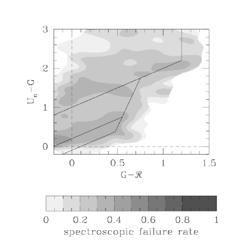
Figure 2.— The fraction of spectroscopically observed galaxies for which we were unable to measure a redshift as a function of $U_{n}G{\cal R}$ color.

4. COLOR SELECTION AT $1.0\lower 2.15277pt\hbox{$\;\buildrel<\over{\sim}\;$}Z\lower 2.15277pt\hbox{$\;\buildrel<\over{\sim}\;$}1.5$

4.1. Balmer-break selection at $z\simeq 1.0$

Most galaxies have a break in their spectra at $\lambda_{\rm rest}\sim 4000$Å that is produced by a combination of Hydrogen Balmer-continuum absorption in the spectra of B, A, and F stars and CaII H&K absorption in the spectra of F, G, and K stars. The relative strengths of the Balmer and 4000Å breaks depends upon the mixture of stellar types in a galaxy—younger galaxies have stronger Balmer breaks and older galaxies have stronger 4000Å breaks—but few galaxies have no break at all (Figure 3).

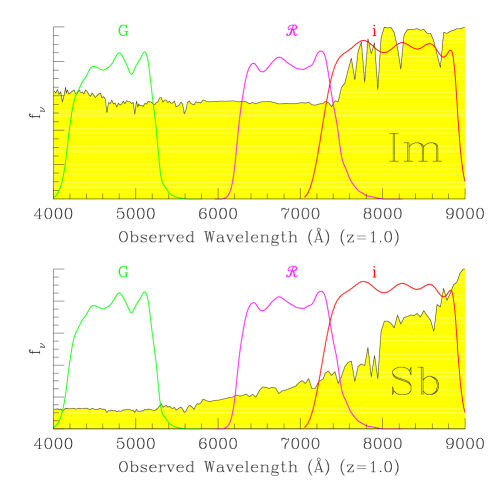
Figure 3.— The Balmer and 4000Å breaks. Younger galaxies, represented by the “Im” model spectrum (§ 2), have a Balmer break near 3700Å due to Hydrogen Balmer absorption in the spectra of B, A, and F stars. Older galaxies, represented by the “Sb” model spectrum (§ 2), have 4000Å CaII H&K breaks. These breaks give distinctive $G{\cal R}i$ colors to galaxies at $z\sim 1$.

Figure 1 suggests that this break should give distinctive broadband colors to galaxies at $z\sim 1$. At no other redshift will a strong break between ${\cal R}$ and $i$ be accompanied by a flatter spectrum at bluer wavelengths. Our first guess at photometric selection criteria targeting galaxies at $z\sim 1$ was inspired by figure 4, which shows the $G{\cal R}i$ colors of model galaxies at various redshifts (§2) and of stars in our own galaxy. Spectroscopic follow-up of objects with colors that are characteristic of $z\sim 1$ galaxies and distinct from the colors of other objects should produce a redshift survey consisting primarily of galaxies at $z\sim 1$. These objects lie to the right of the diagonal line in figure 4, suggesting

$${\cal R}-i\geq 0.4(G-{\cal R})+0.2,\quad\quad G-{\cal R}\leq 1.8\quad\quad\quad\mathbf{[FN]}$$ (1)

as reasonable criteria for identifying the $z\sim 1$ galaxies in deep $G{\cal R}i$ images. These criteria are called “FN” in our internal naming convention and may be referred to by that name in subsequent publications.

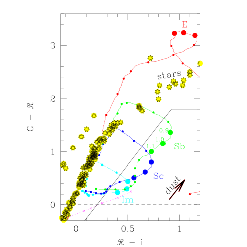
Figure 4.— Expected locations of stars and galaxies on a $G{\cal R}i$ two-color diagram. The stars are from Gunn & Stryker (1983). The curved tracks show the colors of model galaxies of different spectral types (see § 2) at various redshifts, starting at $z=0$ and increasing clockwise. Circles mark redshift intervals of $dz=0.1$; large circles mark $z=0.9,1.0,1.1$. Dust reddening (Calzetti 1997) to $E(B-V)=0.15$ was assumed. The arrow indicates the color change corresponding to $\Delta E(B-V)=0.2$ for an Sc galaxy at $z=1.0$. One would expect to find galaxies at $z\sim 1$ and little else to the right of the diagonal line. Since the line is nearly parallel to the reddening vector, this conclusion does not depend strongly on galaxies’ assumed dust content. Sb galaxies fall to the right of the line even for redshifts significantly larger than $z=1$, but higher-redshift Sbs are not a major component of our sample because Sb spectral types are significantly less common than Sc at $z\sim 1$ (cf. figure 5) and because higher redshift sources are fainter and less easily able to satisfy any apparent-magnitude limit. The dotted line shows the colors of a model galaxy at $z=1.0$ that has been forming stars at a constant rate. Crosses mark its colors after 3,10,30,100,300,1000 Myr of star-formation. The galaxy becomes redder as it ages and begins to satisfy our selection criteria for $t\lower 2.15277pt\hbox{$\;\buildrel>\over{\sim}\;$}30$Myr.

Even if galaxies at $z\sim 1$ had colors that matched the models perfectly, and even if we suffered no photometric errors, figure 4 makes it clear that some galaxies at $z\sim 1$ would not satisfy the selection criteria above. These are galaxies with extreme star-formation histories. At one extreme are galaxies whose present star-formation rates are much lower than their past average. A survey of star-forming galaxies at $z\sim 1$ (such as ours) will be only negligibly affected by their omission. Of more potential concern are galaxies at the opposite extreme, galaxies with present star-formation rates much higher than their past average. The spectra of these galaxies are dominated by light from massive O stars—by stars whose atmospheres are too hot to contain significant amounts of neutral Hydrogen—and consequently they do not have Balmer breaks. Since a Balmer break begins to be discernible when a star-formation episode has lasted longer than the typical $\sim 10^{7}$ yr lifetime of an O star, and since most star formation in the local universe (e.g., Heckman 1997) and at $z\sim 3$ (e.g., Papovich et al. 2001; Shapley et al. 2001) occurs in episodes that last substantially longer than $10^{7}$ yr, we suspected that our reliance on the Balmer-break in our selection criteria would not cause us to miss significant numbers of star-forming galaxies at $z\sim 1$.

In order to obtain empirical support for our proposed selection criteria (equation 1), we began in August 1995 to obtain $G{\cal R}i$ images in fields with completed or ongoing magnitude-limited redshift surveys. Four fields were chosen: the 00^h53 field of Cohen et al. (1999), the Hubble Deep Field (Williams et al. 1996; Cohen et al. 2000), the 14^h18 field of Lilly et al. (1995), and the 22^h18 field of Cowie et al. (1996) and Lilly et al. (1995). Spectroscopic redshifts have been published for 1312 objects in these fields combined. The published coordinates for these objects were sufficient for us to easily and unambiguously identify 1138 of them with objects in our images. 738 of the objects are in the HDF-N, where spectroscopic follow-up has been especially deep and complete; their colors and redshifts are shown in figure 5. One can see that the bulk of known galaxies at $z\sim 1$ have $G{\cal R}i$ colors that satisfy our selection criteria.

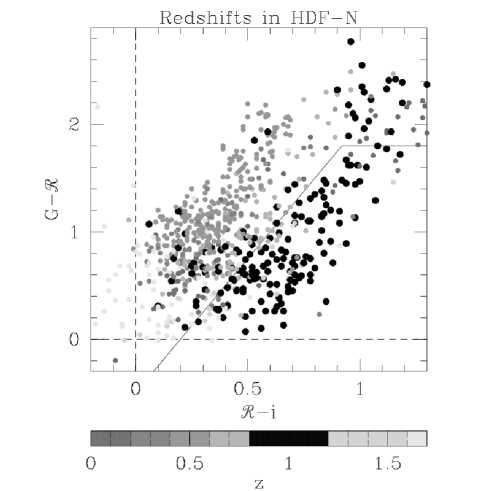
Figure 5.— Observed redshifts of objects with different $G{\cal R}i$ colors. The data are taken from various magnitude-limited surveys in the HDF-N; see text. Known galaxies at $z\sim 1$ have colors similar to our expectations from figure 4. The solid line shows the $z\sim 1$ selection criteria of equation 1.

The galaxies at $0.85<z<1.15$ that do not satisfy our $G{\cal R}i$ selection criteria can be crudely grouped into three classes. Please refer to figure 5. First, there are the handful of galaxies with ${\cal R}-i\simeq 0.9$, $G-{\cal R}\lower 2.15277pt\hbox{$\;\buildrel>\over{\sim}\;$}2.0$. These galaxies have rest-frame colors nearly identical to those of local ellipticals (see figure 4). They are objects that formed the bulk of their stars in the past and are no longer forming stars at a significant rate. Their absence from a color-selected survey of star-forming galaxies is expected and harmless. Second, there are objects with colors identical to those of low redshift galaxies but with reported spectroscopic redshifts $z\simeq 1.0$. Some of these objects may have unusual star-formation histories or large photometric errors or exceptionally strong emission lines, and some may have incorrectly measured spectroscopic redshifts. Third, there are objects with measured colors that lie just outside the Balmer-break color selection window. These galaxies may have been scattered out of our selection window by photometric errors, which are typically $\sim 0.2$ magnitudes in both $G-{\cal R}$ and ${\cal R}-i$. Their absence from a Balmer-break selected survey can be largely corrected with statistical techniques described in Adelberger (2002,2004).

Figure 6 presents the data of figure 5 in a way that may be easier to grasp. We produced one alternate realization of figure 5’s data by adding to each galaxy’s $G{\cal R}i$ colors a Gaussian deviate with standard deviation $\sigma=0.1$ that is similar to the color’s measurement uncertainty. After repeating this procedure numerous times, we concatenated the alternate realizations into a large list of $G-{\cal R}$, ${\cal R}-i$, $z$ triplets, and then calculated, for each point in the $G{\cal R}i$ plane, the fraction of galaxies with those colors in the large list that had redshift $0.85<z<1.15$. Figure 6 shows the result. As anticipated, the portion of the $G{\cal R}i$ plane that is dominated by star-forming galaxies at $z\sim 1$ is approximately described by equation 1. One exception is the region near $G-{\cal R}\sim 2.8$, ${\cal R}-i\sim 0.9$, which is populated primarily by galaxies at $z\sim 1$ but lies outside our selection window. It would be easy to modify the window to include this region, but, as mentioned above, galaxies at $z\sim 1$ with these colors do not account for much of the star-formation density. We chose to ignore them. Readers interested in stellar mass rather than star-formation rate might choose differently.

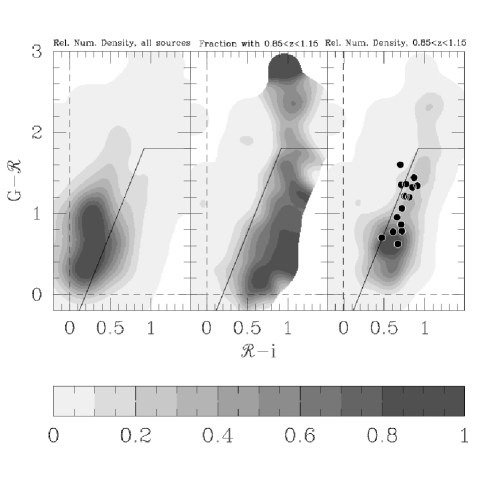
Figure 6.— Left panel: The distribution of colors for all objects in deep $G{\cal R}i$ images of the HDF-N. Middle panel: The probability that an object has $0.85<z<1.15$ as a function of $G{\cal R}i$ color. Right panel: The distribution of $G{\cal R}i$ colors for objects with $0.85<z<1.15$ in the HDF-N. Superimposed are the colors of the 16 ISO $15\mu$m sources with $0.84<z<1.15$ in this field (see Adelberger & Steidel 2000 and references therein; 41 of the 46 ISO sources in this field have measured spectroscopic redshifts, so it is unlikely that there is a large number of spectroscopically unidentified ISO sources at $z\sim 1$ with colors significantly different from these). These extremely dusty sources are among the most rapidly star-forming galaxies at $z\sim 1$, but their optical colors are sufficiently similar to those of more normal galaxies that they satisfy our selection criteria (equation 1, solid line in all panels). There is little evidence that our UV-based selection criteria bias our samples against the dustiest galaxies, a point that has been more laboriously made by Adelberger & Steidel (2000) and Adelberger (2001).

Ideal color-selection criteria would be perfectly complete and perfectly efficient; they would be satisfied by every galaxy in the targeted redshift interval and only by galaxies in the targeted redshift interval. Figure 6 shows that in practice the goals of completeness and efficiency are incompatible. Photometric errors and intrinsic variations in the spectra of galaxies cause galaxies inside the redshift interval $0.85<z<1.15$ to have a wide range of $G{\cal R}i$ colors. In some cases these colors are identical to those of galaxies at other redshifts. If we wanted our color-selected survey to be as complete as possible, we would want to make our selection box very large so that it would include even galaxies with large photometric errors or abnormal spectral shapes, but this improvement in completeness would come at the price of admitting more galaxies at the wrong redshifts and it would therefore decrease our efficiency. To quantify how closely our selection criteria satisfied the conflicting goals of completeness and efficiency, we used the magnitude-limited surveys discussed above to calculate two quantities. $\alpha$, the completeness coefficient, is equal to the fraction of galaxies at $0.85<z<1.15$ in the magnitude limited surveys whose colors satisfied equation 1. $\beta$, the efficiency coefficient, is equal to the fraction of magnitude-limited survey objects in the selection box of equation 1 whose measured redshift satisfied $0.85<z<1.15$.

Table 2 lists $\alpha$ and $\beta$, with and without weighting by the galaxies’ apparent luminosities through various filters. Our completeness depends on wavelength. Samples selected through equation 1 are especially complete for the bluest galaxies: the $U_{n}$-weighted column shows that approximately $85$% of the $U_{n}$ (rest-frame $1800$Å) luminosity density detected at $0.85<z<1.15$ in magnitude-limited surveys is produced by galaxies that satisfy the selection criteria. The completeness falls towards redder wavelengths, where the total $z\sim 1$ luminosity density receives larger contributions from older galaxies whose spectra are less dominated by star formation, but even at rest-frame $4500$Å (observed $z$-band) approximately $70$% of the luminosity density at $0.85<z<1.15$ is produced by galaxies whose colors satisfy equation 1. Because our color-selected catalogs extend to magnitudes significantly fainter than those of the magnitude-limited surveys, the detected luminosity density at $z\sim 1$ in our survey is far higher than in the magnitude-limited surveys. The completeness fractions above apply only to the magnitude range ${\cal R}\lower 2.15277pt\hbox{$\;\buildrel<\over{\sim}\;$}24$ where the surveys overlap.

Table 2Color-selection Efficiency, $1\lower 1.50694pt\hbox{$\;\buildrel<\over{\sim}\;$}z\lower 1.50694pt\hbox{$\;\buildrel<\over{\sim}\;$}1.5$

Name	$\alpha,\beta$	$\alpha_{U},\beta_{U}$	$\alpha_{i},\beta_{i}$	$\alpha_{z},\beta_{z}$	Reference	$N_{\rm cand}$	$N_{\rm z}$
$0.85<z<1.15$:
00h53	0.73,0.55	0.95,0.55	0.77,0.55		Cohen et al. 1999	34	168
HDF-N	0.67,0.55	0.81,0.57	0.67,0.49	0.65,0.51	Cohen et al. 2000	166	676
14h18	0.53,0.67	0.60,0.56	0.57,0.64		Lilly et al. 1995	15	123
22h18	0.65,0.46	0.87,0.67	0.67,0.50		Cowie et al. 1996	24	171
median	0.66,0.55	0.84,0.57	0.67,0.53	0.65,0.51
$1.0<z<1.5$:
HDF	0.80,0.53	0.84,0.60	0.78,0.53	0.77,0.54	Cohen et al. 2000	100	676

In the fall of 1997 we began to add occasional $z\sim 1$ galaxy candidates to our Lyman-break galaxy slitmasks. By the spring of 1999 we had settled on our selection criteria (equation 1) and were devoting entire slitmasks to Balmer-break galaxies. Figure 7 shows the overall redshift distribution of the objects observed to date. Excluding the handful of galaxies with $z<0.4$, whose unexpected colors usually resulted from abnormally strong nebular emission lines, the mean redshift is $\langle z\rangle=1.02$ and the r.m.s. is $\sigma_{z}=0.15$.

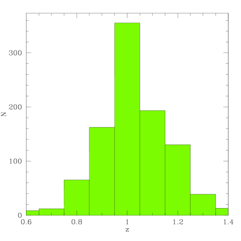
Figure 7.— The redshift histogram the spectroscopically observed sources in our fields whose colors satisfied the selection criteria of equation 1.

4.2. Balmer-break selection at higher redshifts

In principle it would be easy to use similar color-selection criteria to find galaxies at almost arbitrarily high redshifts. In practice there is little reason to pursue this selection strategy beyond the redshift $z\sim 1.5$ where the Balmer-break leaves the optical window; near this redshift bluer spectral features are beginning to enter the optical window and by exploiting these one can continue to take advantage of well-developed CCD detector technology.

Little thought is required to extend the Balmer-break selection to $z\sim 1.5$. Consider figure 8, for example, which shows the expected $G{\cal R}z$ colors of galaxies at different redshifts. The color cuts

$${\cal R}-z\geq 0.8(G-{\cal R})+0.3\quad\quad\quad G-{\cal R}<1.8$$ (2)

isolate galaxies at $1.0<z<1.5$ from the foreground and background populations. Figure 9, calculated in an analogous manner to figure 6, confirms that objects in the HDF with these colors tend to lie at redshifts $1.0<z<1.5$. Table 2 lists the completeness parameters $\alpha$ and $\beta$ for these selection criteria. Approximately $80$% of the known luminosity density at redshifts $1.0<z<1.5$ and observed wavelengths $3000\lower 2.15277pt\hbox{$\;\buildrel<\over{\sim}\;$}\lambda\lower 2.15277pt\hbox{$\;\buildrel<\over{\sim}\;$}9500$Å in the HDF is produced by galaxies whose colors satisfy equation 2. These numbers should be treated with some caution, since the incompleteness of the HDF magnitude-limited spectroscopy strongly skews the observed redshift distribution towards the lower end of the range $1.0<z<1.5$. Nevertheless we hope to have demonstrated that Balmer-break selection allows one to create reasonably complete catalogs of star-forming galaxies throughout the redshift range $1.0\lower 2.15277pt\hbox{$\;\buildrel<\over{\sim}\;$}z\lower 2.15277pt\hbox{$\;\buildrel<\over{\sim}\;$}1.5$.

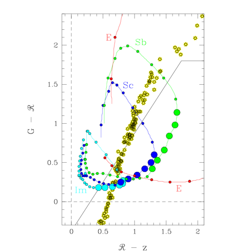
Figure 8.— The expected $G{\cal R}z$ colors of stars and galaxies. The symbols are as in figure 4, except here large dots mark the colors of model galaxies with $E(B-V)=0.15$ at $z=1.0$, 1.1, 1.2, 1.3, 1.4, 1.5 and the solid line shows the selection criteria of equation 2.

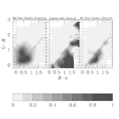
Figure 9.— Similar to figure 6, except results are shown for $G{\cal R}z$ selection of galaxies with $1.0<z<1.5$ rather than $G{\cal R}i$ selection of galaxies with $0.85<z<1.15$.

5. COLOR SELECTION AT $1.9\lower 2.15277pt\hbox{$\;\buildrel<\over{\sim}\;$}Z\lower 2.15277pt\hbox{$\;\buildrel<\over{\sim}\;$}2.7$

Figure 1 shows that the absence of a strong break in the optical window is a distinguishing characteristic of galaxies at $z\sim 2$. Ruling out the existence of a break requires photometry through at least the five filters shown in the figure, but we wanted to devise selection criteria that required imaging through only three. We chose to use the $U_{n}G{\cal R}$ filters for reasons of convenience; our ongoing Lyman-break galaxy survey was producing numerous deep $U_{n}G{\cal R}$ images that we wanted to use for other purposes.

Since the targeted redshift range $1.9<z<2.7$ is similar to the redshift range $2.6<z<3.4$ of the Lyman-break survey, we derived our initial estimates of the $UG{\cal R}$ colors of galaxies at $1.9<z<2.7$ from the observed colors of Lyman-break galaxies. For this we used a sample of 70 Lyman-break galaxies that had spectroscopic redshifts and measured photometry through the $U_{n}G{\cal R}JK_{s}$ bandpasses. 37 of the galaxies were taken from Shapley et al. (2001) and 33 from Papovich et al. (2001). Following the approach outlined in those papers, each galaxy’s photometry was fit with model spectral energy distributions (SEDs) that had a range of star-formation histories and dust reddenings. We found the best-fit SED for every galaxy in the sample, redshifted the best-fit SEDs to $z=1.5$, $z=2.0$, and $z=2.5$, and calculated their $U_{n}G{\cal R}$ colors as described in § 2. This produced an estimate of the $U_{n}G{\cal R}$ colors that each Lyman-break galaxy would have had if its redshift were $z\sim 2$ rather than $z\sim 3$ (figure 10). Star-forming galaxies at $z\sim 2$ should have $U_{n}G{\cal R}$ colors similar to these.

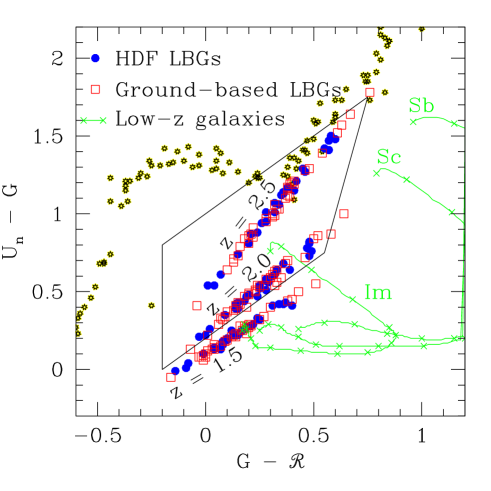
Figure 10.— The expected $U_{n}G{\cal R}$ colors of stars and of star-forming galaxies at various redshifts. Circles and squares mark the colors that would result from shifting the observed SEDs of Lyman-break galaxies at $z\sim 3$ to $z=1.5$, 2.0, 2.5. Data are from Papovich et al. (2001; HDF) and Shapley et al. (2001; ground-based). Curved tracks show the expected colors of model galaxies (§ 2) at lower redshifts, starting at $z=0$ and increasing clockwise to $z=1.5$. Crosses mark redshift intervals of $dz=0.1$. The Sb and Sc tracks move off the plot at $z\sim 0.2$–0.3 and re-enter at $z\sim 0.7$–1.0. Stars represent Galactic stars from Gunn & Stryker (1983). The trapezoid is our selection window (equation 3) for galaxies with $1.9\lower 2.15277pt\hbox{$\;\buildrel<\over{\sim}\;$}z\lower 2.15277pt\hbox{$\;\buildrel<\over{\sim}\;$}2.7$.

Useful color-selection criteria must not only find galaxies at the targeted redshifts but also avoid those at other redshifts. Galaxies at significantly higher redshifts will have extremely red $U_{n}-G$ colors due to the strong Lyman break. They are unlikely to be confused with galaxies at $z\sim 2$. The tracks on figure 10 show the colors of model galaxies at lower redshifts. We considered the templates Im, Sb, Sc from § 2 and reddened each to $E(B-V)=0.15$ with dust that followed a Calzetti (1997) extinction curve. At $0.3\lower 2.15277pt\hbox{$\;\buildrel<\over{\sim}\;$}z\lower 2.15277pt\hbox{$\;\buildrel<\over{\sim}\;$}1.0$ galaxies have red $G-{\cal R}$ colors due to the redshifted Balmer/4000Å breaks and are easily distinguished from galaxies at $z\sim 2$. At lower and higher redshifts the potential for confusion is greater. Young galaxies (type Im) at $z<0.3$ and $1.5<z<1.9$ have $U_{n}G{\cal R}$ colors sufficiently similar to those of galaxies at $1.9<z<2.7$ that a clean separation is impossible given $U_{n}G{\cal R}$ images alone. Our selection criteria were designed in large part to mitigate this contamination.

To learn how to design a selection window that would exclude as many interloping galaxies as possible, we began in the fall of 1996 to obtain spectra of objects with colors similar to those we expected for galaxies at redshift $z\sim 2$. Figure 11 shows how galaxies’ $U_{n}G{\cal R}$ colors depend on their redshifts. In addition to the galaxies whose redshifts we measured for this purpose, the figure includes all galaxies from the Lyman-break survey of Steidel et al. (2003) and all galaxies from the magnitude-limited surveys and our Balmer-break survey described in § 4. Figures 12 and 13 present these data in a way that may be easier to understand. Both are constructed in a similar manner to figure 6. Figure 12 shows the typical $U_{n}G{\cal R}$ colors of galaxies at $z<1$. These were the galaxies that we hoped to exclude from our sample. Figure 13 shows as a function of $U_{n}G{\cal R}$ color the relative number density of sources (left panel), the fraction of objects that lie in the redshift range of interest $1.9<z<2.7$ (middle panel), and the implied relative number density of sources in the same redshift range (right panel). Because no existing magnitude-limited surveys contain significant numbers of galaxies at these redshifts, the right panel was calculated by multiplying the left and center panels together.

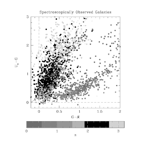
Figure 11.— Spectroscopic redshifts of objects with different $U_{n}G{\cal R}$ colors. The hooked shaped is produced by the transition from Balmer/4000Å absorption in the spectra of galaxies at $z\lower 2.15277pt\hbox{$\;\buildrel<\over{\sim}\;$}1$ to Lyman absorption in the spectra of galaxies at $z\lower 2.15277pt\hbox{$\;\buildrel>\over{\sim}\;$}2.5$. Galaxies at intermediate redshifts have neutral $U_{n}G{\cal R}$ colors; those with $2.0\lower 2.15277pt\hbox{$\;\buildrel<\over{\sim}\;$}z\lower 2.15277pt\hbox{$\;\buildrel<\over{\sim}\;$}2.5$ tend to lie within the region enclosed by the trapezoid (equation 3).

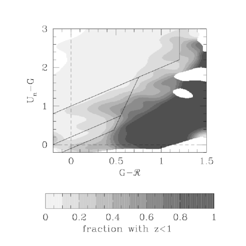
Figure 12.— The fraction of sources that have spectroscopic redshift $z<1$ as a function of $U_{n}G{\cal R}$ color. The solid lines enclose the Lyman-break selection window of Steidel et al. (2003) and the two $1.4<z<2.7$ selection windows discussed below (equations 3 and 6).

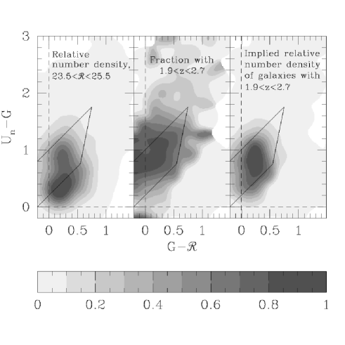
Figure 13.— Left panel: The distribution of colors for all objects with ${\cal R}>23.5$ in deep $U_{n}G{\cal R}$ images of the HDF-N. Middle panel: The observed probability that an object with ${\cal R}>23.5$ has redshift $1.90<z<2.70$ as a function of $U_{n}G{\cal R}$ color. Right panel: The product of the left and middle panels. This shows the implied colors of objects with $1.90<z<2.70$. The trapezoid in all panels shows the selection criteria of equation 3.

The following selection criteria were inspired by the shape of the contours on these plots, by our requirement that galaxies of all LBG-like spectral types have a finite probability of satisfying the criteria, and by our desire to leave no gap between these criteria and the Lyman-break selection criteria of Steidel et al. (2003):

$$G-{\cal R} \geq -0.2$$

$$U_{n}-G \geq G-{\cal R}+0.2\quad\quad\quad\quad\quad\quad\lower 8.61108pt\hbox{\bf[BX]}$$

$$G-{\cal R} \leq 0.2(U_{n}-G)+0.4$$

$$U_{n}-G < G-{\cal R}+1.0.$$ (3)

These criteria are called “BX” in our internal naming convention and may be referred to by that name in subsequent publications.

Figure 14 shows the redshift distribution of randomly selected objects whose colors satisfy these criteria. Excluding sources with $z<1$, the mean redshift is $\bar{z}=2.22$ and the standard deviation is $\sigma_{z}=0.34$.

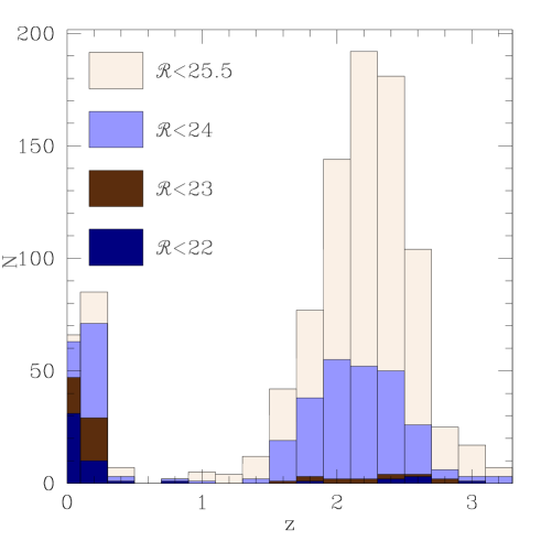
Figure 14.— The observed redshift distribution of objects whose colors satisfy equation 3. Stars are included in the bin containing $z=0$; they make up 4.6% of the sample but only 0.9% of the sample fainter than ${\cal R}=23.5$.

As could be anticipated from figure 10, the Balmer break in low redshift galaxies can sometimes be confused with the Lyman-$\alpha$ forest absorption in the spectra of galaxies at $z\sim 2$. The resulting contamination of our sample is severe at magnitudes ${\cal R}<23$ but negligible by ${\cal R}=25.5$. Restricting the sample to ${\cal R}>23.5$ provides a crude but effective way of eliminating low-redshift interlopers.

One can roughly estimate the completeness coefficients $\alpha$ and $\beta$ for the sample as follows. Let $P(x,y)$ be the probability that a randomly chosen galaxy with $23.5<{\cal R}<25.5$ and colors $G-{\cal R}=x$ and $U_{n}-G=y$ has a redshift that lies in the range $1.9<z<2.7$, let $n(x,y)$ be proportional to the observed number density of galaxies with $23.5<{\cal R}<25.5$ that have colors $G-{\cal R}=x$ and $U_{n}-G=y$, and let $I(x,y)$ be equal to 1 if the color $G-{\cal R}=x$, $U_{n}-G=y$ satisfies equation 3 and to 0 otherwise. Then the probability than an object with $23.5<{\cal R}<25.5$ at $1.9<z<2.7$ will satisfy our selection criteria is

$$\alpha=\int\!\!dx\,dy\,\,P(x,y)n(x,y)I(x,y)\,\,\,\Bigg{/}\,\,\,\int\!\!dx\,dy\,\,P(x,y)n(x,y)$$ (4)

and the probability that an object with $23.5<{\cal R}<25.5$ that satisfies our selection criteria will lie at $1.9<z<2.7$ is

$$\beta=\int\!\!dx\,dy\,\,P(x,y)n(x,y)I(x,y)\,\,\,\Bigg{/}\,\,\,\int\!\!dx\,dy\,\,n(x,y)I(x,y).$$ (5)

The functions $P(x,y)$ and $n(x,y)$ are shown in figure 13. Numerically integrating equations 4 and 5 yields the estimates $\alpha=0.64$, $\beta=0.70$. Roughly two-thirds of galaxies with $1.9<z<2.7$ satisfy our selection criteria, and roughly two-thirds of the galaxies that satisfy our selection criteria lie at $1.9<z<2.7$. The result could have been anticipated to a large extent from the redshift histogram shown in figure 14.

6. COLOR SELECTION AT $1.4\lower 2.15277pt\hbox{$\;\buildrel<\over{\sim}\;$}Z\lower 2.15277pt\hbox{$\;\buildrel<\over{\sim}\;$}2.1$

Our approach towards defining selection criteria at these redshifts differs little from our approach at higher redshift. As redshift decreases from $z=2$, galaxies become bluer in $U_{n}-G$ because a smaller fraction of their observed-frame $U_{n}$ emission is absorbed by the Lyman-$\alpha$ forest. Otherwise their optical colors are largely unchanged. One would expect galaxies with $1.4<z<2.1$ to lie just below our $1.9<z<2.7$ selection window (equation 3) in the $U_{n}G{\cal R}$ plane. We began exploratory spectroscopy of galaxies in this part of the $U_{n}G{\cal R}$ plane in the fall of 1997. Observations continued sporadically until the spring of 2003. Figure 15 shows that these observations largely conformed to our expectations. The following selection criteria were inspired by the shape of the contours on this plot, by our requirement that galaxies of all LBG-like spectral types have a finite probability of satisfying the criteria (see figure 10), and by our desire to leave no gap between these criteria and the selection criteria of equation 3:

$$G-{\cal R} \geq -0.2$$

$$U_{n}-G \geq G-{\cal R}-0.1\quad\quad\quad\quad\quad\quad\lower 8.61108pt\hbox{\bf[BM]}$$

$$G-{\cal R} \leq 0.2(U_{n}-G)+0.4$$

$$U_{n}-G < G-{\cal R}+0.2.$$ (6)

These criteria are called “BM” in our internal naming convention and may be referred to by that name in subsequent publications.

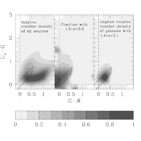
Figure 15.— Similar to figure 6, except the targeted redshift range is $1.4<z<2.1$, the ${\cal R}>23.5$ criteria has been removed, and the trapezoids show the selection criteria of equation 6.

The completeness coefficients $\alpha$ and $\beta$ for these selection criteria, estimated with the approach of equations 4 and 5, are listed in table 3. Roughly $42$% of galaxies with $1.4<z<2.1$ and ${\cal R}<25.5$ satisfy the selection criteria, and roughly $46$% of the objects with ${\cal R}<25.5$ that satisfy the criteria are galaxies with $1.4<z<2.1$. Figure 16 shows the observed redshift distribution of the sources whose colors satisfied equation 6. Excluding sources with $z<1$, the mean redshift is $\bar{z}=1.70$ and the standard deviation is $\sigma_{z}=0.34$. As figure 10 shows, galaxies’ $U_{n}G{\cal R}$ colors do not change by a large amount between $z=1.0$ and $z=1.5$, and as a result the redshift distribution has a significant tail extending to $z\sim 1$. This low-redshift tail can be eliminated to a large extent, if $z$ band photometry is available, by excluding from the sample any objects whose colors satisfy the $1.0<z<1.5$ selection criteria of equation 2. See figure 17. Subsequent papers may refer to this combination of color-selection criteria as “BMZ.”

Table 3Color-selection Efficiency, $1.4\lower 1.50694pt\hbox{$\;\buildrel<\over{\sim}\;$}z\lower 1.50694pt\hbox{$\;\buildrel<\over{\sim}\;$}2.7$

Redshift	$\alpha,\beta$
$1.4<z<2.1$:	0.42,0.46
$1.9<z<2.7$:	0.64,0.70

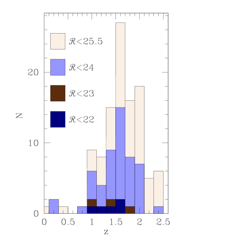
Figure 16.— The redshift distribution of randomly selected objects whose colors satisfy equation 6.

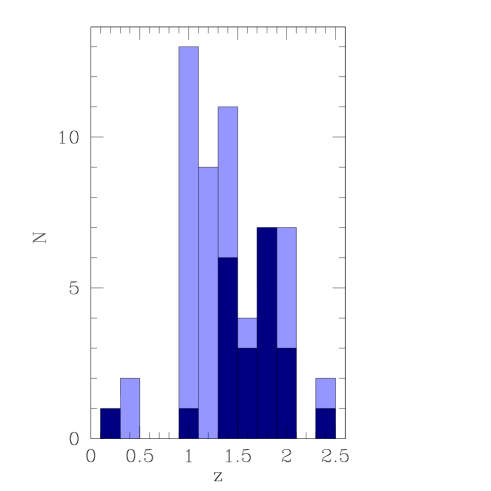
Figure 17.— Light histogram: the redshift distribution of spectroscopically observed objects in the HDF-N whose colors satisfy equation 6. The stellar contamination rate is about 1%. Dark histogram: the redshift distribution of HDF-N objects whose colors satisfy equation 6 but not equation 2.

7. $U_{n}G{\cal R}$ COLOR SELECTION AT ANY REDSHIFT $1<z<3$

The previous two sections presented color-selection criteria tuned to the two arbitrary redshift ranges $1.4<z<2.1$ and $1.9<z<2.7$. Some projects may require a sample of galaxies with a similar but slightly different range of redshifts, e.g., $1.7<z<2.3$. Minor adjustments to the selection criteria we have presented can tune them to this redshift range or others. To help readers estimate how to adjust our criteria to produce samples with a desired range of redshifts, we show in figure 18 the observed median redshift as a function of $U_{n}G{\cal R}$ color of galaxies with ${\cal R}>23.5$ in our spectroscopic sample. Roughly aligning the edges of a selection box with this plot’s contours will produce reasonably good selection criteria tuned to arbitrary redshifts within the interval $1\lower 2.15277pt\hbox{$\;\buildrel<\over{\sim}\;$}z\lower 2.15277pt\hbox{$\;\buildrel<\over{\sim}\;$}3$. Some spectroscopic follow-up will be required to verify the median redshift of the sources and to place limits on the sample’s contamination by stars and low-redshift galaxies.

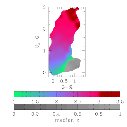
Figure 18.— Median redshift of spectroscopic sources as a function of $U_{n}G{\cal R}$ color. Galaxies from the $U_{n}G{\cal R}$-selected spectroscopic sample described in this paper, from the Lyman-break survey of Steidel et al. (2003), and from the magnitude-limited surveys listed in § 4 were placed into bins with $\Delta(U_{n}-G)=0.1$, $\Delta(G-{\cal R})=0.1$ and the median redshift was calculated for each bin. The resulting array of median redshift vs. $U_{n}G{\cal R}$ color was then smoothed by a Gaussian with $\sigma_{U_{n}-G}=\sigma_{G-{\cal R}}=0.1$ to produce this plot. The slow change of median redshift with color makes it easy to devise selection criteria that target arbitrary redshift ranges within the larger span $1<z<3$.

8. SUMMARY AND DISCUSSION

It is often asserted that studying galaxies at redshifts $1<z<3$ will be tremendously difficult. The optical spectra of galaxies near the middle of this redshift range contain neither the strong spectral breaks that are sometimes thought to be necessary for effective photometric selection nor the strong emission lines Ly-$\alpha$ or [OII]$\lambda 3727$ that are sometimes thought to be crucial for spectroscopic identification. The supposed difficulty of galaxy observations causes many to refer to this redshift range as the spectroscopic desert or high place of sacrifice (Bullock et al. 2001).

We are sceptical. The optical colors of galaxies at redshifts $1<z<3$ are distinctive. We showed in sections 4, 5, and 6 that these galaxies are easy to locate in deep images using simple color-selection criteria (equation 1 for $0.9<z<1.1$, equation 2 for $1.0<z<1.5$, equation 3 for $1.9<z<2.7$, and equation 6 for $1.4<z<2.1$). Once they have been found their redshifts are no harder to measure than those of comparably bright galaxies at slightly higher or lower redshift. This is due in large part to the strength of their interstellar absorption lines. With an appropriately chosen spectroscopic set-up, redshifts are as easy to measure from absorption lines as from the Lyman-$\alpha$ or [OII]$\lambda$3727 emission lines. The point is illustrated by figure 19; during our surveys we obtained as many redshifts per hour of observing time at $1.5<z<2.5$ as at the higher redshifts where Lyman-$\alpha$ is more easily observed. That was possible only because we knew the approximate redshifts of our sources in advance and could optimize our choice of spectrograph and its configuration accordingly. We could not have measured a redshift for many of the galaxies at $1.5<z<2.5$ with a spectrograph that lacked the good UV throughput of LRIS-B. See Steidel et al. (2004) for a more detailed discussion.

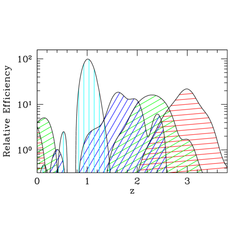
Figure 19.— Scaled redshift distributions of objects selected with equations 1, 6, and 3, and with the $z\sim 3$ Lyman-break selection criteria of Steidel et al. (2003). The actual redshift histogram of each sample was divided by the spectroscopic observing time devoted to the sample. All histograms were then multiplied by the same arbitrary constant and fit with a cubic spline. The area under each curve is proportional to the number of spectroscopic redshifts we measured per hour with the LRIS spectrograph. Galaxy spectroscopy is not much harder at $1<z<3$ than at higher or lower redshifts—as long as the spectrograph has good UV throughput.

Two to three nights spent imaging a single field with a UV-sensitive $40^{\prime}\times 40^{\prime}$ camera on a 4m telescope is sufficient to detect $\sim 2\times 10^{4}$ galaxies that satisfy one set of the $1<z<3$ color-selection criteria that we have presented. A major benefit of color-selected spectroscopy is that it lets one draw statistically significant conclusions from this large number of high-redshift galaxies without having to measure a redshift for every one. For example, the $\sim 1000$ spectroscopic redshifts we have measured for objects whose colors satisfy equation 1 tell us, with high precision, what the redshift distribution must be for the large ensemble of objects in the $40^{\prime}\times 40^{\prime}$ image whose colors satisfy equation 1. One can use this knowledge to derive the luminosity function or spatial clustering strength of galaxies at $z\sim 1$ from the list of photometric candidates alone. Because the redshift distribution of photometric candidates does not depend strongly on magnitude for faint galaxies (figure 20), it should be possible to use purely photometric observations to learn about the properties of the numerous high-redshift galaxies that are too faint for spectroscopy. This may be best use of our $z\sim 1$ color-selection criteria, since the brightest galaxies at this redshift are routinely detected in the large and ongoing spectroscopic surveys of Davis et al. (2003) and Le Fevre et al. (2003).

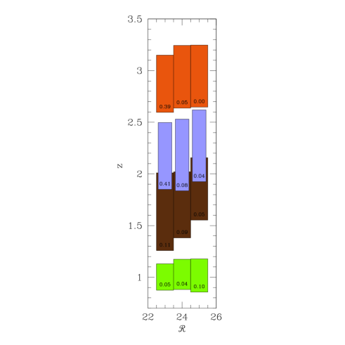
Figure 20.— Redshift distributions as a function of apparent magnitude. Shaded regions show the mean $\pm 1\sigma$ redshift range for objects of different apparent magnitudes whose colors satisfy (from bottom to top) equations 1, 6, 3 and the $z\sim 3$ Lyman-break selection criteria of Steidel et al. (2003). The $1\sigma$ interval was calculated after excluding interlopers with $z<0.4$ from the $z\simeq 1.0$ sample and interlopers with $z<1$ from the other samples. The number in each box indicates the fraction of sources that were excluded. This fraction depends strongly on magnitude for some samples, but otherwise the redshift distributions are insensitive apparent magnitude. It is therefore reasonable to assume, when the interloper fraction is small, that faint photometric candidates will have the same redshift distribution as brighter candidates with spectroscopic redshifts. The weak trend of higher redshifts for (apparently) fainter objects results from the change in luminosity distance.

The weakness of color-selected surveys is that not all galaxies at the targeted redshifts will satisfy the adopted selection criteria. A high level of completeness at the targeted redshifts can be obtained only at the price of admitting large numbers of galaxies at the wrong redshifts. With the simple selection criteria we presented, observers will find more than $\sim$ one-half of the galaxies brighter than the magnitude limit at the redshift of interest and will waste no more than $\sim$ one-half of their observing time observing objects at other redshifts. 50% completeness is not ideal, but the problem is less severe than one might imagine. First, a star-forming galaxy at $1<z<3$ that does not satisfy one of our color-selection criteria will likely satisfy another. Consider galaxies with redshift $1.8<z<2.2$ and magnitude ${\cal R}<25.5$, for example. Equation 4 implies that only 63% of them will satisfy the $1.9<z<2.7$ selection criteria of equation 3. But an additional 26% will satisfy the $1.5<z<2.0$ selection criteria of equation 6, and an additional 5% will satisfy the Lyman-break galaxy selection criteria of Steidel et al. (2003). A total of 94% of photometrically detected galaxies with $23.5<{\cal R}<25.5$ and $1.8<z<2.2$ will satisfy one of the $U_{n}G{\cal R}$ selection criteria we have presented. By conducting redshift surveys with each of these criteria, one can reduce the incompleteness to a reasonably low level. Second, even if a survey adopts only one of our selection criteria, much of the incompleteness can be corrected in a statistical sense. The incompleteness is largely due to the photometric errors in our color measurements, which are not small compared to the size of our color-selection window. Many galaxies whose true colors lie inside our selection window will have measured colors that lie outside the window; many galaxies whose measured colors lie inside will have true colors that lie outside. The result is a broad, bell-shaped redshift histogram rather than a boxcar extending from the minimum to the maximum targeted redshift. Because photometric uncertainties are easy to characterize with Monte-Carlo simulations, their contribution to our incompleteness is easy to understand and correct. Adelberger (2002,2004) explains in detail.

In any case, all observational strategies require some compromise between efficiency and completeness, and the compromises of color selection do not look bad compared to the alternatives. Suppose one were interested in studying galaxies at $0.85<z<1.15$. By obtaining a spectrum of every galaxy brighter than ${\cal R}=24.0$ in an image one would be certain to produce a statistically complete sample of galaxies at $z\sim 1$ to this magnitude limit, but over 80% of the observing time would have been spent on objects at the wrong redshifts (e.g., Cohen et al. 2000). If one were willing to tolerate 15% incompleteness in observed $U_{n}$ luminosity density, one could cull spectroscopic targets with the color criteria of equation 1 and reduce the required observing time by more than a factor of three (see table 2). As redshift increases the benefits of color-selection become more obvious. Only one object out of 50 in the magnitude limited survey of Cohen et al. (2000) had a redshift $1.9<z<2.7$. If one wished to study galaxies at these redshifts with a magnitude limited survey the required observing time would be 33 times longer than if one color-selected targets with equation 3 (see table 3). A project that could be completed in 1–2 years with color-selection would require a lifetime of observing with standard magnitude-limited techniques. The $\sim 30$% incompleteness of color-selected surveys does not seem a high price to pay.

Magnitude-limited optical surveys are not the only alternative to color-selected optical surveys. Many have advocated finding galaxies at $1<z<3$ with photometry outside of the optical window. We chose to develop criteria that relied solely on optical photometry because ground-based optical imagers offer an unrivaled combination of high sensitivity, high spatial resolution, and large fields-of-view. This is an advantage that is difficult to overcome. Surveys at other wavelengths have their strengths—near-IR observations should provide a more complete census of older stars (e.g., Franx et al. 2003, Rudnick et al. 2003) and far-IR/sub-mm observations should yield more reliable estimates of star-formation rates—but the fact remains that an investigator given two nights on an older 4m optical telescope can create a photometric sample of high-redshift galaxies larger than all existing samples at other wavelengths combined. It seems likely to us that much of what we will learn about galaxies at $1<z<5$ in the coming decade will come from large optical surveys selected with color criteria similar to ours.

Attentive readers may have recognized that the derivation of these criteria did not require much thought. That is exactly the point. The value of this paper, if any, lies not in our photometric selection criteria themselves but in the proof that large samples of galaxies at $1<z<3$ can be created with trivial techniques that rely solely on ground-based imaging and well-developed CCD technology. The spectroscopic desert is a myth.

KLA is deeply grateful for unconditional support from the Harvard Society of Fellows. It will be missed. CCS and AES were supported by grant AST0070773 from the U.S. National Science Foundation and by the David and Lucile Packard Foundation. NAR is supported by the National Science Foundation. This research made use of the NASA/IPAC Extragalactic Database (NED), which is operated by the Jet Propulsion Laboratory, California Institute of Technology, under contract with the National Aeronautics and Space Administration. The authors wish to extend special thanks to those of Hawaiian ancestry for allowing telescopes and astronomers upon their sacred mountaintop. Their hospitality made our observations possible.

References

- (1)
- (2) Adelberger, K. L. & Steidel, C. C. 2000, ApJ, 544, 218
- (3) Adelberger, K. L. 2002, PhD thesis, California Institute of Technology
- (4) Adelberger, K. L. 2004, in preparation
- (5) Adelberger, K.L. 2001, in Starburst Galaxies: Near and Far, eds. L. Tacconi & D. Lutz, Heidelberg: Springer-Verlag, 318 304, 15
- (6) Baum, W.A. 1962 in IAU Symp 15, Problems of Extra-galactic Research, ed. G. C. McVittie (New York: Macmillan), 390
- (7) Bruzual, G. & Charlot, S. 1993, ApJ, 405, 538
- (8) Budavári, T., Szalay, A., Connolly, A., Csabai, I., & Dickinson, M. 2000, AJ, 120, 1588
- (9) Bullock, J.S., Dekel, A., Kolatt, T.S., Primack, J.R., & Somerville, R.S. 2001, ApJ, 550, 21
- (10)
- (11) Calzetti, D. 1997, AJ, 113, 162
- (12)
- (13) Chapman, S.C., Blain, A.W., Ivison, R.J., & Smail, I. 2003, Nature, 422, 695
- (14) Cohen, J.G., Hogg, D.W., Pahre, M.A., Blandford, R., Shopbell, P., & Richberg, K. 1999, ApJS, 120, 171
- (15) Cohen, J.G., Hogg, D.W., Blandford, R., Cowie, L.L., Hu, E., Songaila, A., Shopbell, P. & Richberg, K. 2000, ApJ, 538, 29
- (16)
- (17) Cowie, L.L., Songaila, A., Hu, E.M., & Cohen, J.G. 1996, AJ, 112, 839
- (18) Davis, M. et al. 2003, SPIE, 4834, 161
- (19) Dickinson, M. & Giavalisco, M. 2002, in Bender R., Renzini A., eds., ESO Astrophysics Symposia Series, The Mass of Galaxies at Low and High Redshift, Springer-Verlag, Berlin, 324
- (20) Dickinson, M., Papovich, C., Ferguson, H.C., & Budavári, T., 2003, ApJ, 587, 25
- (21) Fernández-Soto, A., Lanzetta, K.M., Chen, H.-W., Pascarelle, S.M., & Yahata, N. 2001, ApJS, 135, 41
- (22) Franx, M. et al. 2003, ApJL, 587, 79
- (23)
- (24) Gunn, J.E. & Stryker, L.L. 1983, APJS, 52, 121
- (25)
- (26) Hogg, D.W. et al. 1998, AJ, 115, 1418
- (27) Koo, D.C. 1985, AJ, 90, 418
- (28)
- (29) LeFevre, O. et al. 2003, SPIE, 4834, 173
- (30) Lilly, S.J., Hammer, F., Le Fevre, O., & Crampton, D. 1995, ApJ, 455, 75
- (31) Loh, E. D., & Spillar, E. J. 1986, ApJ, 303, 154
- (32) Madau, P. 1995, ApJ, 441, 18
- (33)
- (34) Meier, D. L. 1976, ApJ, 207, 343
- (35)
- (36) Papovich, C., Dickinson, M., & Ferguson, H.C. 2001, ApJ, 559, 620
- (37)
- (38) Rowan-Robinson, M. 2003, MNRAS, in press
- (39) Rudnick, G. et al. 2003, ApJ, submitted (astro-ph/0307149)
- (40) Shapley, A.E., Steidel, C.C., Adelberger, K.L., Dickinson, M., Giavalisco, M., & Pettini, M. 2001, ApJ, 562, 95
- (41) Steidel, C. C., Giavalisco, M., Pettini, M., Dickinson, M., & Adelberger, K. L. 1996, ApJL, 462, 17
- (42) Steidel, C. C., Adelberger, K. L., Giavalisco, M., Dickinson, M., & Pettini, M. 1999, ApJ, 519, 1 & Kellogg, M. 1998, ApJ, 492, 428
- (43) Steidel, C.C., Adelberger, K.L., Shapley, A.E., Pettini, M., Dickinson, M., & Giavalisco, M. 2003, ApJ, 592, 728
- (44)
- (45) Williams, R.E. et al. 1996, AJ, 112, 1335
- (46)