Mass and Light in the Supercluster of Galaxies MS0302+17

We investigate the supercluster MS0302+17 ($z\approx 0.42$) using weak lensing analysis and deep wide field $BVR$ photometry with the CFH12K camera. Using $(B-V)$ vs. $(V-R)$ evolution tracks we identify early-type members of the supercluster, and foreground ellipticals. We derive a R band catalogue of background galaxies for weak lensing analysis. We compute the correlation functions of light and mass and their cross-correlation and test if light traces mass on supercluster, cluster and galaxy scales.
We show that the data are consistent with this assertion. The $\zeta$-statistic applied in regions close to cluster centers and global correlation analyses over the whole field converge toward the simple relation $M/L=300\pm 30\,h_{70}\,({\rm M/L})_{\odot}$ in the B band. This independently confirms the earlier results obtained by Kaiser et al. (1998).
If we model dark matter halos around each early-type galaxy by a truncated isothermal sphere, we find that a linear relation $M\propto L$ still holds. In this case, the average halo truncation radius is $s_{*}\lesssim 200\,h^{-1}_{70}\,{\rm kpc}$ close to clusters cores whereas it reaches a lower limit of $\sim 300\,h^{-1}_{70}\,{\rm kpc}$ at the periphery. This change of $s_{*}$ as a function of radial distance may be interpreted as a result of tidal stripping of early type galaxies. Nevertheless the lack of information on the spatial distribution of late-type galaxies affects such conclusions concerning variations of $s_{*}$.
Though all the data at hand are clearly consistent with the assumption that mass is faithfully traced by light from early-type galaxies, we are not able to describe in detail the contribution of late type galaxies. We however found it to be small. Forthcoming wide surveys in UV, visible, and near infrared wavelengths will provide large enough samples to extend this analysis to late-type galaxies using photometric redshifts.

1 Introduction

Detailed investigations of superclusters of galaxies help to understand the late evolution of large scale structures in the transition phase between the linear and non-linear regime. In contrast to wide field cosmological surveys that primarily draw the global structure formation scenario, supercluster studies focus on more detailed descriptions of the physical properties of baryonic and non-baryonic matter components on tens of kiloparsec to tens of megaparsec scales. Within the evolving cosmic web, numerical simulations predict that gas cooling or dark halos and galactic interaction processes start prevailing against large scale gravitational clustering and global expansion of the universe (Vogeley et al. 1994; Bond, Kofman & Pogosyan 1996; Kauffmann et al. 1999). Small scale dissipation processes transform early relations between the apparent properties of large scale structures and those of the underlying matter content. The comparison of mass-to-light ratios and of the mass and light distributions as a function of local environment between supercluster and cluster scales may therefore reveal useful imprints on the physical processes involved in the generation of linear and non-linear biasing (Kaiser 1984; Bardeen et al. 1986).

The properties of large scale structures (LSS) can be characterized by optical, X-ray, Sunyaev-Zeldovitch effect and weak lensing observations. These techniques are widely used on clusters and groups of galaxies (see e.g. Hoekstra et al. 2001; Carlberg et al. 1996; Bahcall, Lubin, & Dorman 1995), but their use is still marginal at larger scales. Superclusters of galaxies are therefore still poorly known systems. Besides early investigations (Davis et al. 1980; Postman, Geller, & Huchra 1988; Quintana et al. 1995; Small et al. 1998), all recent studies on Abell901/902 (Gray et al. 2002) (hereafter G02), Abell222/223 (Proust et al. 2000; Dietrich, Clowe, & Soucail 2002), MS0302+17 (Fabricant et al. 1994; Kaiser et al. 1998) (hereafter K98), Cl1604+4304/Cl1604+4321 (Lubin et al. 2000) or RXJ0848.9+4452 (Rosati et al. 1999) show that superclusters of galaxies are genuine physical systems where gravitational interactions between clusters of galaxies prevail. There is however no conclusive evidence that superclusters are gravitationally bound systems.

Numerical simulations show that supercluster properties may be best characterised by the shape and matter content of the filamentary structures connecting neighboring groups and clusters. Unfortunately, the physical properties of these filaments are still poorly known, though their existence at both low and very high redshift seems confirmed by a few optical and X-ray observations (Möller & Fynbo 2001; Durret et al. 2003).

An alternative approach has been proposed by K98, G02 and Clowe et al. (1998) who used weak lensing analyses. While gravitational lensing has been used on a large sample of clusters of galaxies (See e.g. Mellier 1999; Bartelmann & Schneider 2001, and references therein), its use at supercluster scales is still in its infancy. It has been pioneered by K98 and Kaiser et al. (1999) who used V and I band data obtained at CFHT to probe the matter distribution in the MS0302+17 supercluster. Similar analyses were done later by G02 for the A901/902 system using wide field images obtained with the WiFi instrument mounted at the MPG/ESO 2.2 telescope in La Silla Observatory. Wilson et al. (2001b) applied similar techniques to “empty” fields. In these papers, the projected mass density, as reconstructed from the distortion field of background galaxies, has been compared to the light distribution on several scales. All these studies conclude that there is a strong relation between the light of early type galaxies the and dark matter distributions as if all the mass was traced by early type galaxies.

Over scales of a few megaparsecs, K98 found that the dark matter does not extend further than the light emission derived from the early-type galaxies sample. According to their study, there is almost no mass associated with late type galaxies. In contrast, G02 argued that there is some, but its fraction varies from one cluster to another, leading to a lower and more scattered $M/L$ than K98 found. This discrepancy may be explained if either the two superclusters are at different dynamical stages, or their galaxy populations differ (fraction of early/late type galaxies).

The reliability of their results may however strongly depend on systematic residuals. It is worth noticing that the weak lensing signal produced by filaments is indeed expected to be difficult to detect because projection effects may seriously dilute the lensing signal (Jain, Seljak, & White 2000). Therefore, systematics produced by technical problems related to the way both groups analyzed their data may also be a strong limitation. It is therefore important to confirm early K98 conclusions from an independent analysis, and possibly go further in order to take into account the properties of dark halos. In particular, it is interesting to compare the halo properties (size, velocity dispersion) of cluster galaxies with those of field galaxies. MS0302+17 seems a generic and almost ideal $z\approx 0.42$ supercluster configuration for such an astrophysical study because it is composed of three very close rich clusters (mean projected distance $\sim 15\arcmin$).

In this paper, we describe the investigation of this system. Using new data sets obtained in B, V and R at the CFHT with the CFH12K CCD camera, we explore the mass and light distributions in the supercluster area. Since the CFH12K field of view is 1.7 times larger than the UH8k camera, the three clusters and most of their periphery are totally encompassed in the CFH12K field and we can even explore whether other clusters lie in the field at the same redshift. A quick visual inspection of the southern cluster (ClS) reveals that it is very dense. The giant arc discovered by Mathez et al. (1992) is visible. Similar arc(let) features are also visible in the northern (ClN) and eastern (ClE) systems, making the MS0302+17 supercluster a unique spectacular lensing configuration, where strong and weak lensing inversions can be done.

This paper is organized as follows. In Sect. 2 we describe the observations that were carried out and reduced. We include details on how both astrometric and photometric solutions were computed. We present a detailed quality assessment of the catalogues, where comparisons to existing deep catalogues are made. In Sect. 3 we explain how object catalogues were produced for supercluster members identification. Sect. 4 presents the weak lensing signal produced by the dark matter component. Sect. 5 shows how these two components cross-correlate. Results are discussed in Sect. 6 and our conclusions and summary are presented in Sect. 7. Throughout this paper we adopt the cosmology $\Omega_{m}=0.3,\quad\Omega_{\Lambda}=0.7,\quad H_{0}=70\,h_{70}\,{\rm km.s}^{-1}{\rm Mpc}^{-1}$, leading to the scaling relation $1\arcmin=333\,h^{-1}_{70}\,{\rm kpc}$ at $z=0.42$.

2 The Data

2.1 Observations and data reduction

The observations of the MS0302+17 supercluster area were obtained on October 12, 1999. They were carried out with the CFH12K camera mounted at the prime focus of the Canada-France-Hawaii Telescope. The CFH12K mosaic device is composed of $6\times 2$ thinned backside illuminated MIT Lincoln Laboratories CCID20 $2048\times 4096$ CCDs with a $15\,\mu\rm m$ pixel size. The wide field corrector installed at the prime focus provides an average pixel scale of $0\aas@@fstack{\prime\prime}205$ and the whole field of view of the CFH12K camera is $43\aas@@fstack{\prime}2\times 28\aas@@fstack{\prime}9$. Useful details on the camera can be found in Cuillandre et al. (2000) and in McCracken et al. (2003) (hereafter McC03).

The pointings were centered at the reference position RA(2000) = $03^{\rm h}\leavevmode\nobreak\ 05^{\rm m}\leavevmode\nobreak\ 26.00^{\rm s}$ and DEC(2000) = $+17^{\rm o}\leavevmode\nobreak\ 17{\rm{}^{\prime}}\leavevmode\nobreak\ 54{\rm{}^{\prime\prime}}$, so that the CFH12K field of view encompasses the three major clusters of galaxies. Sequences of dithered exposures were obtained in B, V and R filters using small shifts of about 30 arcsec to fill the gaps between the CCDs and to accurately flat field each individual image frame. Table 1 summarizes and assesses the useful observations used in this paper.

The B, V and R data were processed and calibrated at the TERAPIX data center located at IAP. The pre-calibration process was done using the flips package. Photometric and astrometric calibrations, as well as image stacking and catalogue production were done using the current software package available at TERAPIX. The overall pre-reduction (bias and dark subtraction, flat-field calibration), photometric and astrometric calibration as well as image resampling and co-addition follow exactly the same algorithms and steps as in McC03. We refer to this paper for further details.

Table 1: Summary of the observations with total exposure time (+ the number of dithered pointings), seeing and limiting magnitude. Following McCracken et al. (2003), the $AB$ limiting magnitude corresponds to a 50% completeness limit.

Filter	exp. time	Seeing	Limiting
	(seconds)	(arcsec)	Mag
$B_{AB}$	$6\times 600=3600$	0.9	25.75
$V_{AB}$	$6\times 600=3600$	0.9	25.50
$R_{AB}$	$10\times 720=7200$	0.7	26.50

2.2 Photometric calibration

The photometric calibration was done using Landolt star fields SA95 and SA113 (Landolt 1992). The IRAS maps (Schlegel, Finkbeiner & Davis 1998) show that the Galactic extinction is important in this field. The average $E(B-V)=0.125$, leading to extinction corrections in $B$, $V$ and $R$ of 0.508, 0.384 and 0.285 respectively. We adopted the $AB$ magnitude corrections provided by McC03: $B_{AB}=B-0.097$, $V_{AB}=V-0.007$ and $R_{AB}=R+0.218$.

The object photometry was derived using the Magauto parameter of SExtrator (Bertin & Arnouts 1996) for the magnitude and Magaper for the color index, with the V catalogue as reference position, inside a 2 arcsec aperture. The galaxy number counts derived from this photometry peak at $B_{AB}=24.9$, $V_{AB}=24.3$ and $R_{AB}=25.6$. As in McC03, we derived the limiting magnitude by adding simulated stellar sources in the field. The limiting depths at which 50% of these sources are recovered are $B_{AB}=24.9$, $V_{AB}=24.3$ and $R_{AB}=25.6$, in good agreement with the expectations from the McC03 F02 deep exposures, once rescaled to a similar exposure time (see Fig. 1).

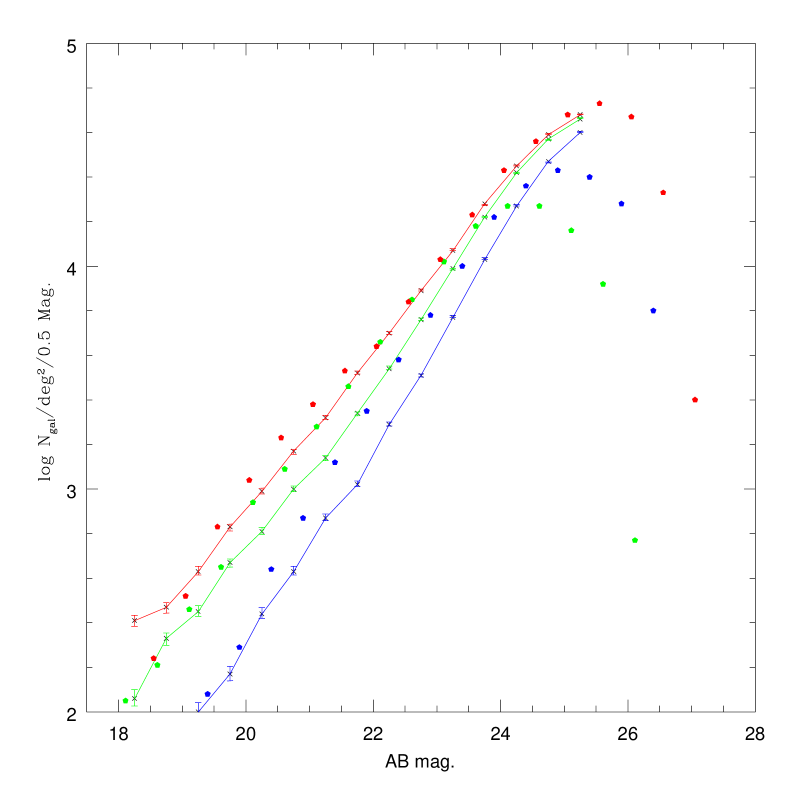
Figure 1: $BVR$ galaxy counts in the MS0302+17 supercluster field. The red, green and blue dots show the galaxy number density in $R$, $V$ and $B$, respectively. The solid red, green and blue lines show the same counts obtained with the same filters on the deep VIRMOS F02 field by McC03. For the bright and faint magnitudes the agreements are excellent. In between, the MS0302+17 counts show a systematic excess that reveals the supercluster populations at $z=0.42$.

The reliability of the photometric calibration was checked by comparing the $B$, $V$ and $R$ galaxy counts to those published for the VIRMOS F02 field by McC03. The supercluster galaxy population contaminates the galaxy number counts. However, as the $B-(B-V)$ and $R-(B-R)$ color-magnitude diagrams show, the bright-end and faint-end galaxy populations are dominated by field galaxies, so we expect the data of the MS0302+17 supercluster and the VIRMOS F02 data to be comparable for these populations. We checked that the counts agree within 0.05 magnitudes with McC03 for the three filters.

We also checked the $(B-V)$ versus $(V-R)$ color-color magnitude of stars, as selected from the SExtractor stellar index. To avoid mixing of galaxies in the sample, we only used bright objects that have a reliable stellar index. The colors are plotted in Fig. 2 (yellow dots) and compared to selected stars on the main sequence and giant-star $(B-V)/(V-R)$ tracks from Johnson (1966). Two populations are clearly visible: the blue stars ($B-V<1.0$) are halo stars, the red ones ($\langle B-V\rangle\simeq 1.3$) are disk M-dwarf stars. The blue population perfectly matches the Main Sequence, but for the red sample we found a systematic offset of $0.1$ in the $(B-V)$ term. A similar discrepancy has already been mentioned by Prandoni et al. (1999). It is likely due to the color correction, which is no longer linear for those stars. The dispersion is easily explained by the intrinsic dispersion of stellar colors and likely from statistical magnitude measurement errors. We therefore conclude that our $(B-V)$ and $(V-R)$ colors have an internal error of $\pm 0.05$ magnitude.

Figure 2: Color-color diagram of bright stellar objects in the MS0302+17 supercluster field. The horizontal and vertical axes are the Johnson $(B-V)$ and $(V-R)$ color indices, respectively. The red and blue dots show the stellar tracks for Main Sequence and Giant stars, as predicted by Johnson (1966). The yellow dots are the color positions of the bright star sample. The figure clearly shows two populations : the blue halo stars ($(B-V)<1.0$) and the red disk M-dwarf stars.

The CCD to CCD calibration errors are in principle minimized since all CCDs are rescaled with respect to the reference CCD$\#$4 that contains several Landolt stars. However, residuals from illumination correction may still bias the calibration. We checked the CCD to CCD stability by comparing the B, V and R galaxy counts. The contamination by cluster galaxies in the field makes this approach difficult. Their effects were minimized by removing the cluster regions from the count estimates. However, since the diffuse supercluster filaments also contaminate the signal, large CCD to CCD fluctuations of the counts still remain. We therefore focused on the faint end part of the magnitude distribution, where the supercluster populations should be negligible. Using these constraints, the average CCD to CCD galaxy count fluctuations in B, V and R are 2.5% in each filter, with peaks of 7.5%. When clusters fields are included and the magnitude range is broadened, the peaks reach 16%. This clearly reveals the presence of clusters populations. Possible residuals from calibration problems are therefore negligible compared to fluctuations expected from Poisson or cosmic variance.

Possible color variations of stars from one CCD to another were checked using a color analysis of 100 stars per chip. We found that they all show similar average $(B-V)$ and $(V-R)$ colors inside the 12 CCDs, within $\pm 0.1$ ($ie\>2\sigma$) and without any systematic color gradient. This confirms, independently of the galaxy counts, that the photometry and our $(B-V)$ and $(V-R)$ colors are stable enough across the field to meet our scientific goals.

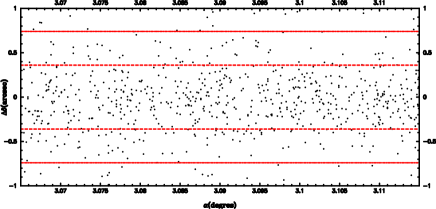
Figure 3: Astrometric calibration of the MS0302+17 field. The top panel shows the residual $\Delta\alpha$ and $\Delta\delta$ between the USNO reference star position and the astrometric solution. The two bottom panels show the $RA$ and $DEC$ residual star position difference as a function of the $RA$ and $DEC$ in the MS0302+17 supercluster field. No trend is visible, showing that astrometry is stable across the whole field of view.

2.3 Astrometric calibration

The astrometric calibration was done using the Astrometrix package developed jointly by the TERAPIX center and Osservatorio di Capodimonte in Naples for wide field images. The algorithms are extensively described in McC03 and Radovich et al. (2003), so we refer to these two papers for further details.

For the MS0302+17 data, the calibration was done using the USNO-A2.0 reference star catalogue (Monet 1998). The astrometric center and tangent point of the CFH12K is $\alpha_{\rm 2000}=03^{\rm h}\leavevmode\nobreak\ 05^{\rm m}\leavevmode\nobreak\ 25.8^{\rm s}$ and $\delta_{\rm 2000}=+17^{\rm o}\leavevmode\nobreak\ 17{\rm{}^{\prime}}\leavevmode\nobreak\ 54{\rm{}^{\prime\prime}}$. Since the $V$ image has much fewer saturated stars than the $R$ image, we preferred to use it as the reference astrometric data, although the $R$ is deeper and has a better seeing. We then cross-correlated the $V$ input catalogue generated by SExtractor to the USNO-A2.0. After rejection of saturated objects, we found 731 stars common to both catalogues. The star sample is homogeneously spread over the CCDs, so that we used 50 to 70 stars per CCD. Fig. 3 shows the residuals between the reference USNO-A2.0 star positions and positions derived from the astrometric solution. The $rms$ coordinate error is $0\aas@@fstack{\prime\prime}45$ (68%) and is similar in both $RA$ and $DEC$ directions ($\Delta\alpha=0\aas@@fstack{\prime\prime}36$, $\Delta\delta=0\aas@@fstack{\prime\prime}30$, respectively). No systematic shift or position gradient is visible. Each $V$ frame was resampled according to the astrometric calibration and then stacked to produce the final $V$ image.

The $B$ and $R$ images are calibrated with respect to the $V$ image. The matching uses detection catalogues generated by SExtractor so the cross-correlation can be done using several thousands of stars and galaxies. Since the $B$, $V$ and $R$ data were obtained during the same night, systematic offsets only correspond to small shifts imposed by the observer, and rotation between each image is negligible. Across such a small field, the atmospheric differential refraction for an airmass ranging between 1.0 to 1.5 produces shifts smaller than $0\aas@@fstack{\prime\prime}4$ between the $B$, $V$ and $R$ image and a chromatic residual that is less than $0\aas@@fstack{\prime\prime}04$ between the $B$ and $R$ image. The $rms$ coordinate errors between the $B$ and $R$ catalogue and the $V$ reference are $0\aas@@fstack{\prime\prime}05$ (68% CL).

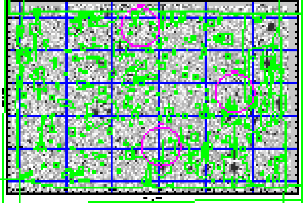
Figure 4: $R$ band image of the MS0302+17 supercluster field used for the light and mass analysis. Coordinates are in J2000. The center point is $RA=03^{\rm h}\leavevmode\nobreak\ 05^{\rm m}\leavevmode\nobreak\ 25.79^{\rm s}$ and $DEC=+17^{\rm o}\leavevmode\nobreak\ 17{\rm{}^{\prime}}\leavevmode\nobreak\ 54.02{\rm{}^{\prime\prime}}$. The field size is $42.9\arcmin\times 29.0\arcmin$ (i.e. $14.2\,h^{-1}_{70}\,{\rm Mpc}\times 9.6\,h^{-1}_{70}\,{\rm Mpc}$ @ $z=0.42$). The 3 arcmin radius circles show the cluster positions of the X-ray emission peaks: ClN, North $03^{\rm h}\leavevmode\nobreak\ 05^{\rm m}\leavevmode\nobreak\ 17.81^{\rm s},\,+17^{\rm o}\leavevmode\nobreak\ 28{\rm{}^{\prime}}\leavevmode\nobreak\ 37.6{\rm{}^{\prime\prime}},\,z=0.425$, ClE, East $03^{\rm h}\leavevmode\nobreak\ 06^{\rm m}\leavevmode\nobreak\ 18.89^{\rm s},\,+17^{\rm o}\leavevmode\nobreak\ 18{\rm{}^{\prime}}\leavevmode\nobreak\ 33.9{\rm{}^{\prime\prime}},\,z=0.418$ and ClS, South $03^{\rm h}\leavevmode\nobreak\ 05^{\rm m}\leavevmode\nobreak\ 31.49^{\rm s},\,+17^{\rm o}\leavevmode\nobreak\ 10{\rm{}^{\prime}}\leavevmode\nobreak\ 16.3{\rm{}^{\prime\prime}},\,z=0.426$. Green polygons define the masked areas that have been removed from the image analysis.

2.4 Final catalogues

Using the calibrated $B$, $V$, and $R$ images, we then produced the final $BVR$ objects catalogue. It contains 28600 galaxies and 1100 stars, as defined according to the SExtractor stellarity index. The common area is composed of 12500 $\times$ 8500 pixels and is 0.343 deg² wide. It corresponds to an angular size of $42\aas@@fstack{\prime}7\times 28\aas@@fstack{\prime}9$ (i.e. $14.2\,h^{-1}_{70}\,{\rm Mpc}\times 9.6\,h^{-1}_{70}\,{\rm Mpc}$ at $z=$0.42) .

For weak lensing analysis we produced another catalogue that only uses the $R$ band image without regard of the $B$ and $V$ data. This image is the deepest one and has the best seeing. The weak lensing catalogue contains more objects than the joined $B$, $V$ and $R$ one. Its properties are detailed in Sect. 4.

CCD defects, gaps or overlap areas between CCDs, bright stellar halos, saturated stars and asteroid track residuals generate spurious features. They are removed from the catalogue using the manual masking process described in van Waerbeke et al. (2000, 2001) as shown in Fig. 4. Field boundaries are also masked, and we finally end up with an effective area of 0.228 deg². The catalogues discussed in the following will only concern this common unmasked part of the field.

3 Supercluster galaxies and light distribution

As shown above, the color information is stable across the field within 0.05 mag accuracy which is sufficient to make a reliable selection of cluster and non-cluster galaxies using colors. The supercluster member selection and the redshift distribution of foreground and background lensed sources were done using color-color diagrams together with the measurement of photometric redshifts.

3.1 Photometric Redshifts vs. Color-Color relation

We first attempted to use $B$, $V$ and $R$ photometry to derive photometric redshifts using the hyperz package (Bolzonella et al. 2000). Details of the method applied to clusters or deep multi-color wide field surveys can be found in Athreya et al. (2002); van Waerbeke et al. (2002); Gavazzi et al. (2003). However, compared to these previous analyses, we only have three bands, which severely reduces the reliability of photometric redshift information. When compared to an “empty” region located westward on the field, the photometric redshifts show an excess of galaxies in the redshift range $\left[0.25-0.65\right]$. The photometric redshift uncertainty ($\sim\pm 0.2$) hampers any detailed redshift investigation of the supercluster galaxies. This noisy redshift information can partially be used for the distinction between foreground and supercluster objects and background lensed galaxies (See Sect. 4).

Fortunately, at redshift $z\approx 0.4$ the typical 4000Å  break spectral feature lies between the $B$ and $R$ filters and can easily reveal early type galaxies. The cluster selection was therefore primarily focused on the red cluster sequence in the color-magnitude diagrams. By using a $B$, $V$ and $R$ color-color diagram of well-defined magnitude limited sample of galaxies for the selection the supercluster members, one can easily isolate co-eval early-type cluster galaxies. We first flagged objects within a 1.5 arcmin radius from the center of each cluster. Fig. 5 shows the $(B-V)$ versus $(V-R)$ color-color diagram. Early-type galaxies concentrate around $1.1\leq(B-V)\leq 1.42$, the supercluster elliptical galaxies at $z=0.42$ having also $0.47\leq(V-R)-0.5(B-V)\leq 0.77$. Objects with a $(V-R)$ color bluer than that band are elliptical galaxies with a lower redshift. Most are in the redshift range $0.1<z<0.4$. Passive evolution tracks for elliptical galaxies kindly provided by D. Leborgne (see Fioc & Rocca-Volmerange 1997) are in excellent agreement with our observations.

The following set of equations summarizes our selection criteria for early-type galaxies. Equations (1a)-(1c) are criteria for supercluster members, whereas (1a)-(1b) and (1d) stand for the selection of foreground early-type galaxies.

$$19\,\leq\,R\,\leq\,23,$$ (1a)

$$1.1\,\leq\,(B-V)\,\leq\,1.42$$ (1b)

$$0.47\,\leq\,(V-R)-0.5(B-V)\,\leq\,0.77$$ (1c)

$$0.2\,\leq\,(V-R)-0.5(B-V)\,\leq\,0.47$$ (1d)

The foreground sample has a mean redshift $z\simeq 0.3$ and contains 770 galaxies, and the supercluster sample contains 750 galaxies. Their luminosity distribution is well centered around $L_{*}$. We did not select ellipticals with $z<0.2$ since they are very few and provide a negligible lensing signal. Elliptical galaxies at $z\geq 0.6$ also have a poor lensing efficiency compared to those at the supercluster redshift.

Our color-color selection method fails to localize bluer late-type galaxies. Thus, we have to keep in mind that the light due to cluster spirals is not taken into account. K98 and Fabricant et al. (1994) argued that $\approx 30\%$ of the total $B$ band rest-frame luminosity is due to late-types, so their contribution, though sizeable, is not expected to be dominant.

We estimated the contamination by field galaxies inside the color-color region of supercluster members. We selected similar galaxies satisfying (1a)-(1c) far from the regions around the three clusters and plotted them in the color-color diagram. The fraction of field galaxies inside the cluster color-color region turns out to be negligible. This efficient selection process expresses the fact that for this redshift $(z\approx 0.4$), the $(B-V)$ and $(V-R)$ colors are reliable filters. In contrast, the lower $(V-R)$ limit used for the foreground subsample selection is more questionable, so we may miss some of the nearest ellipticals. However, since their lensing contribution is small, it has no impact on the interpretation of the weak lensing signal.

Figure 5: Upper left panel: Color-color diagram. The red + signs code for the supercluster objects that lie within 1.5 arcmin of individual clusters. The early-types are concentrated around $(B-V)_{AB}\approx 1.2$. The additional knowledge of $(V-R)$ color provides an efficient selection of supercluster objects at $z\sim 0.4$.    Upper right panel: Color-color diagram that explicitly makes the distinction between supercluster and foreground ellipticals along the $(V-R)$ axis. The variation of $(V-R)$ with redshift along the $(B-V)_{AB}\approx 1.2$ line is well reproduced by predicted passive evolution tracks for ellipticals whatever their formation redshift. We define a foreground subsample centered around $z\approx 0.3$ i.e. inside the lower green lozenge whereas the upper red one encompasses the supercluster ellipticals.    The lower panel shows the corresponding spatial distribution. Supercluster members (red + symbols) are clearly clustered around the three known clusters. Foreground objects (green $\times$ symbols) are clearly less clustered although some clumps are also visible.

3.2 Spatial distribution of light & associated convergence

In this section, we investigate the spatial distribution of supercluster galaxies. We also estimate the foreground contribution to light. The apparent $B_{AB}$ magnitudes are converted into rest-frame luminosities using K-corrections also provided by D. Leborgne. For $z=0.42$ supercluster members, we used $K_{B}=1.88$, and for $z\simeq 0.3$ foreground early-types $K_{B}=1.14$. As detailed in Sect. 4.2, the redshift distribution of lensed sources implies the following critical surface densities: $\Sigma_{\rm crit}(z_{d}=0.42)=2.72\times 10^{14}\,h^{-1}_{70}\,{\rm M}_{\odot}/{\rm arcmin}^{2}$ and $\Sigma_{\rm crit}(z_{d}=0.3)=1.95\times 10^{14}\,h^{-1}_{70}\,{\rm M}_{\odot}/{\rm arcmin}^{2}$.

Instead of computing a filtered luminosity map with Gaussian smoothing, we follow the method of K98, G02 and Wilson et al. (2001b). It consists of weighting the luminosity map by its lensing efficiency (different for foreground and supercluster components). Assuming a constant mass-to-light ratio for supercluster galaxies, the luminosity field at a given position $\@vec{\theta}$ is converted into a mass density field, $\Sigma_{\mathcal{L}}(\@vec{\theta})$. Then it is translated into a convergence $\kappa_{\mathcal{L}}(\@vec{\theta})=\Sigma_{\mathcal{L}}(\@vec{\theta})/\Sigma_{\rm crit}$ field. We finally convert it into a shear field $\gamma(\@vec{\theta})$ and derive a supercluster shear pattern that samples the field according to the source catalogue positions (see Sect. 4.2). From this shear field a new convergence field can be drawn. It has the same field size and shape, the same masking and the same sampling properties as the $\kappa$-map we construct in Sect. 4.3.

The inferred shear field reads :

$$\gamma(\@vec{\theta})=\left[\sum_{i=1}^{N_{\rm lens}}\gamma_{0}(\@vec{\theta}-\@vec{\theta_{i}})\right]*W(\@vec{\theta}),$$ (2)

where $W$ is a 40 arcsec Gaussian smoothing filter, and $\gamma_{0}$ is the shear profile of an individual galaxy. Since we are primarily interested in the collective behavior of galaxies and we are looking at scales $\geq 1$ arcmin, we do not make a further hypothesis about the radial density profiles of galaxy halos. This means that galaxies are equivalent to point masses, so $\gamma_{0}$ simply reads:

$$\gamma_{0}(\theta)=\frac{M}{L}\times\frac{L}{\pi\Sigma_{\rm crit}\theta^{2}}$$ (3)

where $M/L$ is the mass-to-light ratio which is assumed to be the same for all galaxies. The $\gamma\rightarrow\kappa$ inversion is detailed in Sect. 4.3. It turns out that luminosity-weighted $\kappa_{\mathcal{L}}$ and number-density-weighted $\kappa_{N}$ convergence maps are almost proportional. A small deviation from equality appears for the highest contrast values. In this case, $\Delta\kappa_{N}/\kappa_{N}\lesssim\Delta\mathcal{\kappa_{L}}/\mathcal{\kappa_{L}}$ as we expect if the brightest galaxies lie in the densest regions.

Figure 6: Effective convergence maps derived from the luminosities of early type galaxies. The convergence is expressed as $\kappa(\@vec{\theta})=\Sigma(\@vec{\theta})/\Sigma_{\rm crit}$ but the supercluster contribution may be contaminated by foreground galaxies. Panel a) (top) shows the luminosity weighted convergence map of supercluster objects, as inferred from the positions of galaxies in the color-color diagram. Panel b) (bottom) shows the same map with the contribution of the foreground galaxies. The origin coordinate is $RA=03^{\rm h}\leavevmode\nobreak\ 05^{\rm m}\leavevmode\nobreak\ 25.79^{\rm s}$ and $DEC=+17^{\rm o}\leavevmode\nobreak\ 17{\rm{}^{\prime}}\leavevmode\nobreak\ 54.02{\rm{}^{\prime\prime}}$. We applied a $40\arcsec$ wide Gaussian smoothing scale. The two maps are almost similar, confirming that foreground structures along the line of sight do not dominate uncertainties in the error budget. Green levels start at $\kappa=0.0$ and increase linearly with step $0.02$. We assumed a fiducial mass-to-light ratio $M/L=300\,h_{70}\,({\rm M/L})_{\odot}$.

The resulting $\kappa$ from light maps are shown in Fig. 6. The upper panel shows the $\kappa_{\mathcal{L}}$ convergence map for the supercluster objects only, whereas the lower panel shows the modifications produced by addition of foreground structures. The three known clusters are clearly detected and seem to encircle a large underdense region. A diffuse extension, less dense than the clusters, appears westward from the northern cluster (ClN). This extension encompasses two clumps at $\Delta\alpha\sim-8\arcmin$ and $\Delta\alpha\sim-15\arcmin$. Another extension toward the North-West of ClS is partly due to foreground structures. Using the spectroscopic redshift of two member galaxies, K98 argued that this clump probably lies at $z=0.3$ .

4 Weakly Lensed objects sample - Shear analysis

The coherent stretching produced by the weak lensing effect due to the MS0203+17 supercluster is measured using the deep catalogue extracted from the $R$ band image. Its depth and high image quality allow us to lower the detection threshold and to increase the galaxy number density ($\approx$ 25 arcmin^-2), compared to the $B$ and $V$ images. This reduces the Poisson noise of the weak lensing statistics and increases the spatial sampling of the supercluster mass reconstructions. Close galaxy pairs with angular separations less than 5 arcsec are discarded to avoid blended systems that bias ellipticity measurements. The reliability of shape measurements is expected to be as good as the current cosmic shear survey data (van Waerbeke et al. 2001).

4.1 PSF correction

Blurring and distortion of stars and galaxies produced by instrument defects, optical aberrations, telescope guiding, atmospheric seeing and differential refraction are corrected using the PSF of stars over the whole field. Several correction techniques and control of systematic errors have been proposed over the past 10 years (see e.g. Mellier 1999; Bartelmann & Schneider 2001; van Waerbeke & Mellier 2003; Réfrégier 2003). In the following we use the most popular KSB95 method initially proposed by Kaiser, Squires, & Broadhurst (1995). Several teams have already demonstrated that the KSB95 method can correct systematics residuals down to the lower limit shear amplitude expected on supercluster scales (van Waerbeke & Mellier 2003; Réfrégier 2003).

Following KSB95 method, the observed ellipticity components $e^{\rm obs}_{\alpha=1,2}$ are composed of its intrinsic ellipticity components $e^{\rm src}_{\alpha}$, and linear distortion terms that express the instrument and atmospheric contaminations and the contribution of gravitational shear to the galaxy ellipticity. Each ellipticity component is transformed as:

$$e^{\rm obs}_{\alpha}=e^{\rm src}_{\alpha}+P^{\rm g}_{\alpha\beta}g_{\beta}-P^{\rm sm}_{\alpha\beta}q^{*}_{\beta},$$ (4a)

$${\rm with\ \ }P^{\rm g}_{\alpha\beta}=P^{\rm sh}_{\alpha\beta}-P^{\rm sm}_{\alpha\gamma}\left(\frac{P^{\rm sh}}{P^{\rm sm}}\right)_{\gamma\beta}^{*},$$ (4b)

where $g$ is the reduced gravitational shear, $P^{\rm sm}$ is the smear polarizability, $P^{\rm sh}$ the shear polarizability and $P^{\rm g}$ the isotropic circularization contribution to the final smearing. In the following, all these tensors are simplified to half their trace and have been calculated with Imcat tools. $\left(\frac{P^{\rm sh}}{P^{\rm sm}}\right)^{*}$ and $q^{*}$ are quantities that are measured from field stars. Their shape is fitted by a second order polynomial, applied individually to each CCD of the CFH12K camera. Stars are selected in the magnitude-$r_{h}$ plane, as usual. $q^{*}$ is the anisotropic part of the PSF, which is subtracted from galaxy ellipticities. The residual is shown in Fig. 7 . It does not show any peculiar spatial pattern and is consistent with a one percent $rms$ noise.

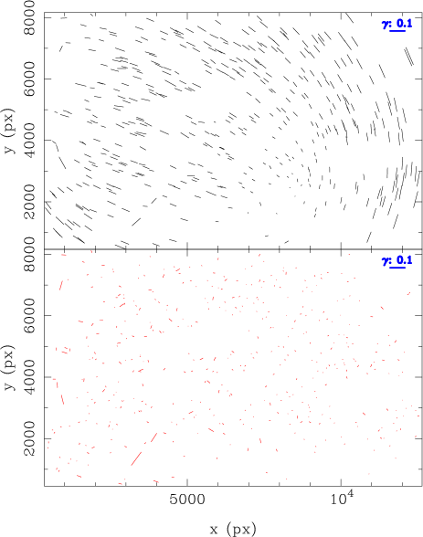
Figure 7: Upper panel : Spatial distribution of stellar ellipticities before (black) and after (red) PSF correction.     Lower panel : The same stellar ellipticities in the $(e_{1},e2)$ plane, uncorrected (black crosses) and corrected (red dots) from PSF anisotropy. The residual $rms$ dispersion around the center is less than one percent.

The smearing part of the PSF contained in the $P^{\rm g}$ term depends on the magnitude of the object and on its size as compared to the seeing disk. To optimally extract $P^{\rm g}$, we derived it from an averaged value over its 70 nearest neighbors in the magnitude$-r_{h}$ plane. Its variance is then used as a weighting scheme for the shear analysis. The weight assigned to each galaxy is finally the inverse variance $\sigma_{e_{i}}^{2}$ of the observed ellipticities :

$$w_{i}=\frac{1}{\sigma_{e_{i}}^{2}}=\frac{P^{g2}}{P^{g2}\sigma_{0}^{2}+\sigma_{i}^{2}},$$ (5)

where $\sigma_{0}=0.3$ is the intrinsic dispersion in galaxy ellipticities and $\sigma_{i}\approx 0.13$ is the observed dispersion of ellipticities over the 70 closest neighbors. A weighted magnitude histogram of the source sample shows that we can select galaxies down to the limiting magnitude $R_{AB}=25.6$. In this subsample, galaxies with a $r_{h}$ smaller than that of stars are discarded.

4.2 Redshift distribution & shear calibration

Because the source sample is deeper than the photometric catalogue, the redshift distribution of background objects cannot be derived from the photometric redshifts calculated with the $B$, $V$ and $R$ data. Nevertheless, for the distinction between foreground and background-lensed objects, we can use a rough limiting redshift estimate.

We chose to reject objects with a $z_{\rm phot}<0.5$. We also discarded the early-type galaxies selected in the color-color diagram of Sect. 3. Finally, we selected background galaxies within the magnitude range : $22.4<R_{AB}<25.6$. The source catalogue contains 22125 galaxies. This corresponds to a number density $n_{\rm bg}\approx 27\,{\rm arcmin}^{-2}$.

The properties of the resulting sample are roughly comparable with those of the sample of van Waerbeke et al. (2001, 2002), though their magnitude cut $I_{AB}<24.5$ instead of $R_{AB}\lesssim 25.6$ as in this work. They inferred the redshift distribution:

$$n(z)=\frac{1}{z_{s}\Gamma(a)}\left(\frac{z}{z_{s}}\right)^{a-1}\,{\rm e}^{-z/z_{s}},$$ (6)

where $a=5/2$, $z_{s}=0.44$ leading to $\bar{z}=az_{s}=1.1$ and $\sigma_{z}=\sqrt{a}z_{s}=0.7$. The median redshift is well approximated by ${\rm Med}(z)\simeq(a-0.33)z_{s}\simeq 0.95$. At the same time, G02 proposed a median redshift $z=1$ for their magnitude cut $R<26$. Using the same analytic form as (6), we found that $a\simeq 1.9$ and $z_{s}\simeq 0.55$ provide a good description of our redshift distribution implying a median redshift ${\rm Med}(z)=1$ and a broader distribution $\sigma_{z}\simeq 0.8$ .
For the supercluster redshift $z_{d}=0.42$ we calculated the mean of the ratio $\beta=\left<D_{ds}/D_{s}\right>$ and the corresponding critical surface density $\Sigma_{\rm crit}=\frac{c^{2}}{4\pi G}\frac{\beta^{-1}}{D_{d}}$, where $D_{d}$, $D_{s}$ and $D_{ds}$ are angular distances between the observer and deflector, observer and sources and deflector and sources, respectively. We found :

$$\begin{split}\beta&=0.49,\\ \Sigma_{\rm crit}&=2.72\times 10^{15}\,h_{70}\,{\rm M}_{\odot}\,{\rm Mpc}^{-2}\\ &=3.02\times 10^{14}\,\,h^{-1}_{70}\,{\rm M}_{\odot}\,{\rm arcmin}^{-2}.\end{split}$$ (7)

For foreground galaxies at $z\sim 0.3$, we found $\beta=0.63$, $\Sigma_{\rm crit}=1.95\times 10^{14}\,\,h^{-1}_{70}\,{\rm M}_{\odot}\,{\rm arcmin}^{-2}$. The redshift distribution of sources is indeed equivalent to a single source plane configuration with redshift $z_{\rm sheet}\approx 0.95$. The depth and the source plane redshift we use are in good agreement with previous ground based analyses like those of Clowe & Schneider (2001, 2002). The uncertainty in the gravitational convergence produced by the redshift distribution of the sources is about 5%, which is much smaller than the error bars we expect from statistical noise due to intrinsic galaxy ellipticities.

4.3 Mass Map

Our mass reconstruction is based on the Kaiser & Squires (1993) (KS93) algorithm. The convergence $\kappa(\@vec{\theta})=\Sigma(\@vec{\theta})/\Sigma_{\rm crit}$ is related to the observed shear field $\gamma(\@vec{\theta})$ through:

$$\kappa(\@vec{\theta})=\int_{\mathbb{R}^{2}}D(\@vec{\theta}-\@vec{\vartheta})^{*}\gamma(\@vec{\vartheta})\,{\rm d}^{2}\@vec{\vartheta},$$ (8)

where $\gamma$ and $D(\@vec{\theta})=\frac{1}{\pi}\frac{-1}{(\theta_{1}-i\theta_{2})^{2}}$ are complex quantities. On the physical scales we are exploring the lensing signal is weak enough so that $\langle e\rangle=\frac{\gamma}{1-\kappa}\simeq\gamma$. The ellipticity catalogue is smoothed with a $\theta_{s}=40\arcsec$ Gaussian filter :

$$\hat{\gamma}(\@vec{\theta})=\frac{1}{N}\sum_{i}w_{i}\,e_{i}\>\exp\left(-\frac{\left(\@vec{\theta}-\@vec{\theta}_{i}\right)^{2}}{2\theta_{s}^{2}}\right),$$ (9)

where $w_{i}$ are the weights defined in Eq. (5) and $N\simeq 2\pi n_{\rm bg}\theta_{s}^{2}\approx 170$ can be viewed as the mean number of sources inside the filter. The resulting convergence map presents correlated noise properties :

$$\langle\kappa_{n}(\@vec{\vartheta})\kappa_{n}(\@vec{\vartheta}+\@vec{\theta})\rangle=\frac{\sigma_{i}^{2}}{8\pi n_{\rm bg}\theta_{s}^{2}}\exp\left(-\frac{(\@vec{\theta}-\@vec{\vartheta})^{2}}{4\theta_{s}^{2}}\right).$$ (10)

$\sigma_{i}\approx 0.42$ is the dispersion in ellipticities of our galaxy sample. $\frac{\sigma_{i}}{\sqrt{8\pi n_{\rm bg}\theta_{s}^{2}}}\simeq 0.016$ characterizes the noise level. The $\kappa$-map reconstruction result is shown in the middle panel of Fig. 8. The bottom panel shows the reconstruction applied to the same galaxy sample, but with the orientation rotated by $45\degr$. It represents the imaginary part of Eq. (8), which should be a pure noise realization if the coherent distortion field is only produced by gravitational lensing.

Figure 8: Upper panel: Mass reconstruction derived from the light distribution emitted by clusters+foreground elliptical galaxies $\kappa_{L}$. This map is almost a reproduction of the b) panel of Fig. 6 with one arcminute filtering scale. Middle panel: Reconstructed dark matter surface density $\kappa(\@vec{\theta})$ using the KS93 inversion technique. Lower panel: Same reconstruction after $45\degr$ rotation of source galaxies. No noticeable patterns due to systematics are visible. In all maps, the shear has been sampled at the observed position of background source galaxies, and the maps suffer the same (edge+mask)-effects. The Gaussian smoothing scale is $1\arcmin$. Levels are the same as in Fig. 6. The overall agreement between panels a) and b) is good.

The three main clusters ClN, ClS & ClE are detected with a high significance. A few substructures with a lower detection significance are also visible. We detail in Sect. 4.4 the various quantities measured for the clusters. A comparison with the X-ray emissivity map displayed on Fig. 1 of K98 shows an excellent agreement. See also Fig. 1 of Fabricant et al. (1994). The clusters are also detected in the $\kappa$-from-light map shown in the top panel of Fig. 8. The clumpy extension detected westward from ClN can be seen in the light map. Another clump located at $03^{\rm h}\leavevmode\nobreak\ 04^{\rm m}\leavevmode\nobreak\ 30^{\rm s}$, $+17^{\rm o}\leavevmode\nobreak\ 15{\rm{}^{\prime}}\leavevmode\nobreak\ 00{\rm{}^{\prime\prime}}$ may be either a foreground structure or an extension toward the west from ClS. This luminous component is visible in the lower panel of Fig. 6 but not in the $\kappa$-map of the top panel. From spectroscopic data, K98 argued that this structure may lie at $z\approx 0.3$. A large void region between the clusters is also apparent in the mass map. When decreasing the smoothing scale, the core of ClE splits into two maxima that are also visible in the higher resolution light map of Fig. 6.

4.4 Properties of clusters

The global properties of the three clusters are explored using integrated physical quantities enclosed within the radius $r_{0}=1\,h^{-1}_{70}\,{\rm Mpc}(=3\arcmin$). For each cluster the center is set to the X-ray emissivity center. Table 2 summarizes the main quantities : the total mass from weak lensing estimates (row 3), the total rest-frame B luminosity emitted by the supercluster early-type galaxy sample (row 4), the inferred mass-to-light ratio (row 5), the “spectroscopic” velocity dispersion compiled from Dressler & Gunn (1992); Fabricant et al. (1994); Carlberg et al. (1996) (row 6), and the velocity dispersion derived from a fit of the weak lensing data to a Singular Isothermal Sphere (SIS) model (row 7): $\kappa(\theta)=\theta_{E}/2\theta$ , where $\theta_{E}=4\pi\left(\frac{\sigma}{c}\right)^{2}\beta$ is the Einstein radius. Rows (8) and (9) are X-ray ROSAT HRI/IPC and ASCA data (Gioia & Luppino 1994; Fabricant et al. 1994; Henry 2000). Row (3) is computed using the densitometric $\zeta-$statistic :

$$\begin{split}\zeta(\theta,\theta_{0})=&\left\langle\kappa(\theta^{\prime}<\theta)\right\rangle-\left\langle\kappa(\theta<\theta^{\prime}<\theta_{0})\right\rangle.\\ =&\frac{2}{1-\left(\theta_{0}/\theta\right)^{2}}\int_{\theta}^{\theta_{0}}\left\langle\gamma_{t}(\theta^{\prime})\right\rangle\,{\rm d}\ln\theta^{\prime}.\end{split}$$ (11)

$\tilde{M}(\theta)=\Sigma_{\rm crit}\pi(D_{d}\theta)^{2}\zeta(\theta,\theta_{0})$ gives a lower bound on the mass contained in the cylinder of radius $\theta$. $\left\langle\gamma_{t}(\theta)\right\rangle$ is the average tangential shear. $\theta_{0}$ is set to 7 arcmin. In practice we used the estimator

$$\hat{\zeta}(\theta,\theta_{0})=\frac{\sum_{i\in I}w_{i}\,e_{t,i}\left(\frac{\theta_{0}}{\theta_{i}}\right)^{2}}{\sum_{i\in I}w_{i}}$$ (12a)

$${\rm Var}(\hat{\zeta})=\frac{\sum_{i\in I}w_{i}^{2}\,\sigma_{i}^{2}\left(\frac{\theta_{0}}{\theta_{i}}\right)^{4}}{\left(\sum_{i\in I}w_{i}\right)^{2}}\ ,$$ (12b)

with $I=\left\{i\mid\theta<\theta_{i}<\theta_{0}\right\}$. The SIS $\theta_{E}$ value is obtained by a $\chi^{2}$ minimisation :

$$\chi^{2}\approx\sum_{i}w_{i}\left(e_{t,i}-\frac{\theta_{E}}{2\theta_{i}}\right)^{2},$$ (13)

where $e_{t}$ is the tangential ellipticity relative to the cluster center. A trivial estimator for $\theta_{E}$ is :

$$\hat{\theta}_{E}=2\frac{\sum_{i}w_{i}e_{t,i}/\theta_{i}}{\sum_{i}w_{i}/\theta_{i}^{2}}.$$ (14)

Note however that this estimator is no longer valid when $\kappa\sim 1$. This means that we have to select galaxies far enough from centers of clusters. Typically, we set $1\arcmin<\theta<7\arcmin$.

Table 2: Summary of cluster properties. $\tilde{M}$ is a lower bound on the cluster mass. $L_{B}$ is the rest-frame blue band luminosity. $M/L$ is the mass-to-light ratio. These three quantities are calculated inside $r_{0}=1\,h^{-1}_{70}\,{\rm Mpc}$. $\sigma_{\rm vel}$ is the kinematic velocity dispersion compiled from spectroscopic data (Dressler & Gunn 1992; Fabricant et al. 1994; Carlberg et al. 1996) whereas $\sigma_{\rm SIS}$ is the velocity dispersion deduced from weak lensing when fitting an isothermal profile for the cluster dark matter halo. Note the two distinct values of $\sigma_{\rm vel}$ for ClS. The lower value from Carlberg et al. (1996) is based on a larger galaxy sample. It is also in better agreement with our estimate. $L_{\rm X,bol}$ is the bolometric X rays luminosity and $T_{\rm X}$ the gas temperature (Gioia & Luppino 1994; Fabricant et al. 1994; Henry 2000).

		ClN	ClS	ClE
(1)	$\alpha_{\rm 2000}$	$03^{\rm h}\leavevmode\nobreak\ 05^{\rm m}\leavevmode\nobreak\ 18^{\rm s}$	$03^{\rm h}\leavevmode\nobreak\ 05^{\rm m}\leavevmode\nobreak\ 31^{\rm s}$	$03^{\rm h}\leavevmode\nobreak\ 06^{\rm m}\leavevmode\nobreak\ 19^{\rm s}$
(2)	$\delta_{\rm 2000}$	$+17^{\rm o}\leavevmode\nobreak\ 28{\rm{}^{\prime}}\leavevmode\nobreak\ 38{\rm{}^{\prime\prime}}$	$+17^{\rm o}\leavevmode\nobreak\ 10{\rm{}^{\prime}}\leavevmode\nobreak\ 16{\rm{}^{\prime\prime}}$	$+17^{\rm o}\leavevmode\nobreak\ 18{\rm{}^{\prime}}\leavevmode\nobreak\ 34{\rm{}^{\prime\prime}}$
(3)	$\tilde{M}(<r_{0})$   $[10^{13}\,\,h^{-1}_{70}\,{\rm M}_{\odot}]$	$33.1\pm 6.7$	$17.9\pm 5.0$	$15.0\pm 5.4$
(4)	$L_{B}(<r_{0})$   $[10^{11}\,h_{70}^{-2}\,{\rm L}_{\odot}]$	$8.3\pm 1.7$	$6.7\pm 1.5$	$11.5\pm 2.0$
(5)	$M/L_{B}$   $[\,h_{70}\,({\rm M/L})_{\odot}]$	$398^{+136}_{-101}$	$266^{+113}_{-85}$	$130^{+57}_{-49}$
(6)	$\sigma_{\rm vel}$   [km s-1]	$821^{+137}_{-94}$	$646\pm{93}$ ($921^{+192}_{-123}$)	$912\pm{200}$
(7)	$\sigma_{\rm SIS}$   [km s-1]	$817^{+83}_{-107}$	$635^{+109}_{-131}$	$595^{+110}_{-133}$
(8)	$L_{\rm X,bol}$   $[10^{44}\,h_{70}^{-2}\,{\rm erg\leavevmode\nobreak\ s}^{-1}]$	$2.75\pm 0.31$	$3.47\pm 0.26$	$1.84\pm 0.36$
(9)	$T_{\rm X}$   [keV]	–	$4.6\pm 0.8$	–

Finally, the rest-frame B-band luminosity is obtained by adding up the luminosities of cluster galaxies with increasing radius. Systematics due to the selection of supercluster members or to contamination dominate the error budget but are small (of order 5% when changing the limits of Eqs. (1) by 10%). To account for cosmic variance, we increased the Poisson noise error by a factor of 1.3, as suggested by Longair & Seldner (1979).

The three clusters differ from one another in terms of mass and luminosity. ClN is the most massive and has the highest mass-to-light ratio. ClS shows apparent properties of a well relaxed cluster. It is highly concentrated with strong lensing features between the two brightest cluster galaxies (Mathez et al. 1992) and a rather high X-ray luminosity. ClE seems more complex: it is the most luminous in the $R$-band although it is the least massive and the least X-ray luminous. Table 2 shows that its kinematical velocity dispersion is much higher than what we infer from weak lensing. The latter estimate is more typical of a cluster mass than the value derived from kinematic data. Hence, ClE is likely not relaxed. We attempted to describe its bimodal structure (see Fig. 6) by fitting two individual isothermal spheres at the location of the luminosity peaks ClE1 ($03^{\rm h}\leavevmode\nobreak\ 06^{\rm m}\leavevmode\nobreak\ 16.5^{\rm s},+17^{\rm o}\leavevmode\nobreak\ 21{\rm{}^{\prime}}\leavevmode\nobreak\ 18{\rm{}^{\prime\prime}}$) and ClE2 ($03^{\rm h}\leavevmode\nobreak\ 06^{\rm m}\leavevmode\nobreak\ 19.9^{\rm s},+17^{\rm o}\leavevmode\nobreak\ 18{\rm{}^{\prime}}\leavevmode\nobreak\ 21{\rm{}^{\prime\prime}}$). We found $\sigma_{\rm ClE1}=312^{+100}_{-215}\,{\rm kms}^{-1}$ and $\sigma_{\rm ClE2}=473^{+84}_{-100}\,{\rm kms}^{-1}$. The fit quality is slightly improved, though the quadratic sum of these individual velocity dispersions is comparable to the single isothermal sphere fit in table 2. Note that ClE is at $z=0.418$ which is a rather high radial distance to the other clusters. The previous studies of Fabricant et al. (1994) and K98 demonstrated that ClE might not be gravitationally bound to the supercluster system.
The X-ray luminosity presents a better correlation with mass than with B-band luminosity. The mass-to-light ratios are rather different but the mean value within 1 megaparsec is $M/L=249^{+41}_{-32}\,h_{70}\,({\rm M/L})_{\odot}$. Within $500\,h^{-1}_{70}\,{\rm kpc}$ we found $M/L=231^{+60}_{-47}\,h_{70}\,({\rm M/L})_{\odot}$ showing that no significant variation with radius is observed. It is worth noticing that values of $M/L$ for individual clusters have a larger scatter.
We found larger errors than K98 for $\tilde{M}$, but our estimates are not based on smoothed mass maps from randomly shuffled catalogs. We directly used galaxy ellipticities in Eq. (12). Hence, our error estimates are more conservative and do not suffer edge + smoothing effects (+ uncontrolled residual correlations).

5 Correlation Analysis

5.1 Linear biasing hypothesis

The high signal to noise ratios and the good resolutions of the light and mass maps are sufficient to explore how light and mass correlate and how these quantities evolve as a function of angular scale. The statistical properties of the relation between dark and luminous matter components can then be analyzed from the cross-correlation of the $\kappa$ mass map with the $\kappa$-from-light map shown in panels b) and a) of Fig. 8.

Let us first assume a simple linear relation between the luminosity from early-type galaxies (cluster+foreground) and the dark matter component. The construction of the $\kappa_{E}$ map for the luminosity of early-type galaxies is detailed in Sect. 3.2. We compute “light” maps again by adopting the same scaling relation as in Eq. (3) with a starting mass-to-light ratio $M/L=300\,h_{70}\,({\rm M/L})_{\odot}$. The linear biasing hypothesis between the dark matter convergence fields $\kappa_{M}$ and $\kappa_{E}$ simply reads :

$$\kappa_{M}=\,\lambda\,\kappa_{E}.$$ (15)

Hence, $300\lambda$ is the mean mass-to-light ratio. If we assume that it is constant with scale and redshift, $\lambda$ is easily constrained by the cross-correlation analysis.

We compute the two-dimensional and azimuthally averaged cross-correlations:

$$C_{AB}(\@vec{\theta})=\langle\kappa_{A}(\@vec{\vartheta})\kappa_{B}(\@vec{\vartheta}+\@vec{\theta})\rangle\equiv\langle\kappa_{A}\kappa_{B}\rangle.$$ (16)

We have to subtract the noise contributions to the correlation functions. Since noise properties of mass and light are not correlated, we only have to calculate the noise autocorrelations :

$$\langle\kappa_{A}\kappa_{A}\rangle\longrightarrow\langle\kappa_{A}\kappa_{A}\rangle-\langle\kappa_{A}\kappa_{A}\rangle_{\rm noise}.$$ (17)

Noise autocorrelation as well as error bars are calculated by a bootstrap technique. We performed 32 randomizations of background galaxy catalogues that mimic the noise properties in $\kappa_{M}$ as predicted by Eq. (10). We also randomly shuffled the shear catalogue calculated with Eq. (2) before smoothing and performing the $\gamma$-to-$\kappa$ inversion. Note also that we discarded the pixels of the convergence maps that lie inside masked areas (see Fig. 4). In these regions, the lack of background galaxies severely increases the noise level. Field boundaries are masked in the same way.
In the following, $\langle\kappa_{M}^{2}\rangle$, $\langle\kappa_{E}^{2}\rangle$, and $\langle\kappa_{M}\kappa_{E}\rangle$ refer to the mass-mass, light-light and mass-light correlation functions respectively. $\langle\kappa_{M}\kappa_{E}\rangle$ shows a maximum at zero lag, which is significant at the 10-$\sigma$ confidence level. The cross-correlation peak is fairly isotropic and well centered on the origin. At zero lag, the normalization parameter of Eq. (15) yields $M/L=277\pm 27\,h_{70}\,({\rm M/L})_{\odot}$.
We thus increased the number of constraints by considering the whole correlation function profile over the 7 inner arcminutes. The $\lambda$ value is derived by performing a global $\chi^{2}$ minimization over the correlation functions, using sufficiently sparse sampling points to reduce the correlations between bins. $\lambda$ satisfies the system:

$$\begin{split}\langle\kappa_{M}^{2}\rangle=&\lambda^{2}\langle\kappa_{E}^{2}\rangle\\ \langle\kappa_{M}\kappa_{E}\rangle=&\lambda\langle\kappa_{E}^{2}\rangle.\end{split}$$ (18)

We found $M/L=286^{+34}_{-39}\,h_{70}\,({\rm M/L})_{\odot}$ with $\chi^{2}/{\rm dof}\simeq 0.88$. The left panel of Fig. 9 shows the $\langle\kappa_{M}\kappa_{E}\rangle$ and $\langle\kappa_{E}^{2}\rangle$ correlation profiles with this mass-to-light ratio normalization. We also observe an excess of light autocorrelation at $\theta\geq 15\arcmin$ which is the characteristic distance between clusters. Note that this bump is enhanced if we only consider supercluster early-types and discard the less clustered foreground contribution.

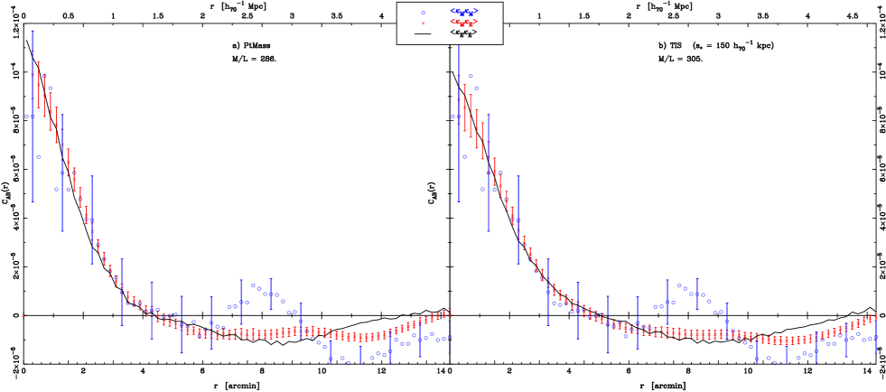
Figure 9: Left panel a) :   $\langle\kappa_{M}^{2}\rangle$, $\langle\kappa_{M}\kappa_{E}\rangle$ and $\langle\kappa_{E}^{2}\rangle$ correlation functions for a mass-to-light ratio $M/L=286\pm 36\,h_{70}\,({\rm M/L})_{\odot}$ that fits the correlation functions at scales $\theta\lesssim 8\arcmin$.   Right panel b) :   Same plot with a TIS halo model (with truncation radius $s_{*}=150\,h^{-1}_{70}\,{\rm kpc}$). With the same assumption $M\propto L$ and a slightly lower $\chi^{2}$, this model also confirms the general conclusion “light traces mass”, provided the truncation radius $s_{*}\lesssim 200\,h^{-1}_{70}\,{\rm kpc}$. Note that the bins are correlated. For clarity, in both cases one fifth of the error bars is displayed for $\langle\kappa_{M}^{2}\rangle$. This coarser sampling roughly shows the required spacing for independent bins.

So far, we find an excellent matching between the $\langle\kappa_{M}^{2}\rangle$, $\langle\kappa_{M}\kappa_{E}\rangle$ and $\langle\kappa_{E}^{2}\rangle$ correlation functions profiles up to $\sim 10$ arcmin. The linear relation (15) turns out to be a good model. As already pointed out by K98, the main conclusion is that early-types galaxies trace the mass. Oscillating patterns around the light autocorrelation appear for $r\geq 8\arcmin$. G02 as well as Wilson et al. (2001b) found similar patterns. They are likely noise artifacts.

As compared to the results of Sect. 4.4, the correlation analysis gives a value for the mass-to-light ratio $\simeq$ 15% higher than that deduced from integrated quantities inside one megaparsec around clusters. The $M/L$ deduced from $\kappa$ maps is insensitive to a constant mass sheet (the so-called mass-sheet degeneracy). Therefore, it is necessary to subtract the mean luminosity contribution in the circular aperture of individual clusters analysis and to only consider the excess of luminosity. We find that within 3 arcmin from the center $M/L=273\pm 47\,h_{70}\,({\rm M/L})_{\odot}$. Therefore, the agreement with the overall correlation analysis is excellent.

The agreement with the K98 results, after rescaling to a flat $\Lambda$ cosmology, is also excellent. Their conclusion that early-type galaxies trace the mass faithfully is therefore confirmed by our analysis. Nevertheless, the authors argued that they saw little evidence for any variation of $M/L$ or ’bias’ with scale. K98 addressed this issue by performing the correlation analysis in the Fourier space by splitting the data into a low and a high frequency bin. They found an increase of $M/L$ ratio with increasing wavelength, ranging from $\sim 180$ at scales $\lesssim 2.5\,h^{-1}_{70}\,{\rm Mpc}$ to $\sim 280$ beyond. The physical meaning of this trend is not clear. Variations of $M/L$ ratio with scale likely indicate underlying physical changes in the relations between mass and light that cannot be interpreted from our simple linear scale-free biasing parameter $\lambda$. In the following, we investigate some models that may explain the $M/L$ variations observed by K98.

5.2 Changing the dark matter halo profile

In Eq. (3), we assumed that dark matter halos of individual galaxies have a little extension compared to the weak lensing filtering scale, so that they can be modeled as point masses with mass proportional to the galaxy luminosity. In this section we study how a more complex dark matter halo profile may change the conclusions of the previous section.
Let us consider a truncated isothermal sphere (TIS) (Brainerd, Blandford, & Smail 1996; Schneider & Rix 1997). The convergence reads

$$\kappa_{\rm TIS}(r)=\frac{b}{2r}\left[1-\frac{r}{\sqrt{r^{2}+s^{2}}}\right].$$ (19)

where $s$ is the truncation radius. When $s\rightarrow\infty$, $b$ reduces to the Einstein radius $\theta_{E}$ of the singular isothermal sphere (SIS). Assuming a $L\propto\sigma^{4}$ scaling relation (Faber & Jackson 1976; Fukugita & Turner 1991) and $M_{\rm tot}=\pi\Sigma_{\rm crit}bs\propto L$, we set

$$\frac{b}{b_{*}}=\left(\frac{\sigma}{\sigma_{*}}\right)^{2}=\left(\frac{L}{L_{*}}\right)^{1/2}\;,\quad\frac{s}{s_{*}}=\left(\frac{L}{L_{*}}\right)^{1/2}\;.$$ (20)

This empirical parameterization is consistent with Wilson et al. (2001a) who assumed $b\propto L^{1/2}$, as well as with Hoekstra, Yee, & Gladders (2003) who found $b\propto L^{0.60\pm 0.11}$ and $s\propto L^{0.24^{+0.26}_{-0.22}}$ leading to $M\propto L^{0.84^{+0.28}_{-0.25}}$.

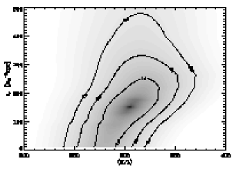
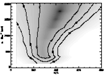
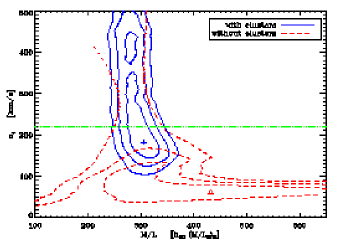
Figure 10: TIS halo modeling. Left : Contour plot showing constraints of mass-to-light ratio and truncation radius of a $L_{*}$ early-type galaxy. The data are consistent with dark matter halos with truncation radius $s_{*}\lesssim 200\,h^{-1}_{70}\,{\rm kpc}$. Middle : same plot when considering the periphery of clusters only, the tendency is reversed and large halos ($s_{*}\gtrsim 400\,h^{-1}_{70}\,{\rm kpc}$) are favored. Right : same constraints interpreted in the $\sigma_{*},M/L$ plane. The two cases with/without cluster masking are overlaied (solid blue / dashed red contours respectively). The horizontal straight line $\sigma_{*}=220\,{\rm km\,s^{-1}}$ is a fiducial value for local elliptical galaxies.

Given that $b_{*}=(M/L)\frac{L_{*}}{\pi s_{*}\Sigma_{\rm crit}}$, we have to constrain the pair $(M/L,s_{*})$, or equivalently $(\lambda=(M/L)/300,s_{*})$. $\lambda$ no longer contributes linearly to the $\kappa_{E}$ expression because of the dependence of $s$ on $L$.
The correlation functions are calculated in the same way as in Sect. 5.1. However, since $s$ is different from one galaxy to another, the resulting correlation function $\langle\kappa_{M}\kappa_{E}\rangle_{\rm TIS}$ (resp. $\langle\kappa_{E}^{2}\rangle_{\rm TIS}$) is no longer the convolution of $\langle\kappa_{M}\kappa_{E}\rangle$ (resp. $\langle\kappa_{E}^{2}\rangle$) by the normalized halo profile (resp. normalized halo profile autocorrelation), making the CPU cost much more important.

Contour plots for $(M/L,s_{*})$ are displayed in the left panel of Fig. 10 yielding $(M/L)_{\rm TIS}=305^{+30}_{-35}\,h_{70}\,({\rm M/L})_{\odot}$ and $s_{*}=150^{+90}_{-150}\,h^{-1}_{70}\,{\rm kpc}$. This value is smaller but still statistically consistent with $s_{*}=264\pm{42}\,h^{-1}_{70}\,{\rm kpc}$ derived by Hoekstra, Yee, & Gladders (2003). However, Hoekstra, Yee, & Gladders (2003) used both early and late type field galaxies and also relaxed the constraint $M\propto L$, making a comparison with our sample difficult. However, because we are using a smoothing scale $\theta_{s}=40\arcsec=220\,h^{-1}_{70}\,{\rm kpc}$, it is only possible to put an upper limit $s_{*}\lesssim 200\,h^{-1}_{70}\,{\rm kpc}$. We therefore cannot rule out that tidal stripping effects in dense environments may decrease the galaxy cut-off radius, as reported by Natarajan, Kneib, & Smail (2002). This point will be discussed in more detail in the next sub-section.

It is also interesting to interpret our results in terms of halo velocity dispersion $\sigma_{*}=c\sqrt{\frac{b_{*}}{4\pi D_{d}}}$ as shown in the right panel of Fig. 10. The Results are consistent with general values for $\sigma_{*}$ (see e.g. Seljak 2002, and references therein).

5.3 Large scales / Periphery of clusters

The results derived in Sect. 5.1 and Sect. 5.2 are in good agreement with those of Sect. 4.4. They confirm that the average mass-to-light ratio of halos is $M/L\approx 300\,h_{70}\,({\rm M/L})_{\odot}$ and that early type galaxies are the primary tracers of dark matter on supercluster scales. Their contribution may however depend also on the local density, and the average value we derived could only reflect a biased signature of the mass-to-light ratio dominated by the three clusters. One could conclude equally well either that early-types trace the mass at all scales with a constant $M/L=300\,h_{70}\,({\rm M/L})_{\odot}$ or that the signal coming from clusters is too strong, and hides more subtle details. This would explain why K98 reported an increasing variation of $M/L$ ratio with increasing scale using two bins of low and high spatial frequencies.

To clarify this, we calculate the correlation functions as above, but we discard the central regions of clusters. More precisely, we set to zero the inner 3 arcmin around each cluster (circles of Fig. 4) to compute the residual correlation produced by the larger scale structures, like filaments and voids. When considering the periphery of clusters only, the amplitude of correlation functions drops by a factor $\sim 3$ showing that most of the signal comes from the clusters.

The constant $M/L$ ratio model with point-mass-like dark matter halo provides a rather bad fit: $\chi^{2}/{\rm dof}\simeq 2.1$. This is significantly worse than for the whole field analysis. The best fit yields $M/L=276\pm 30\,h_{70}\,({\rm M/L})_{\odot}$ and is plotted in the left panel of Fig. 11. For a TIS halo model the goodness-of-fit is significantly improved $(\chi^{2}/{\rm dof}\simeq 0.65)$ when constraining $(M/L,s_{*})$. However, it requires $s_{*}\gtrsim 300\,h^{-1}_{70}\,{\rm kpc}$ and $M/L=280\pm 40$. Note that large values of $s_{*}\sim 1.5\,h^{-1}_{70}\,{\rm Mpc}$ with larger $M/L\sim 400$ are also consistent with the data (see middle panel of Fig. 10). The right panel of Fig. 11 shows such an extended halo profile. It is worth noting that these solutions appear unphysical and may rather indicate that the input model is not well suited.

The fact that halos are more extended outside the cores of clusters is also consistent with the tidal stripping hypothesis. However, as discussed in the following section, this conclusion depends on the input model $M\propto L$ and on the fact that we assumed that all the mass is associated with early-type galaxies. In particular, the contribution of late-type galaxies has been neglected again. The small amount of mass located in low frequency modes in the the outer parts of the supercluster may give an indication that these modes are not well traced by early-type galaxies.

Figure 11: Same as Fig. 9 but with the clusters centers. A large truncation radius TIS model (right panel) provides a better fit than the point-mass halo model (left panel) which does not fit the data well ($\chi^{2}/{\rm dof}\simeq 2.1$). Notice how compared to Fig. 9, the correlation amplitudes drop when the clusters centers are discarded.

6 Discussion

The MS0302+17 supercluster mass distribution, derived from weak lensing analysis of background galaxies, matches the supercluster light distribution of its early type galaxies. The correlation between them is very strong. More precisely the shape of the light-mass cross-correlation profile is in excellent agreement with a simple model where dark matter is directly related to light, assuming a constant mass-to-light ratio.
We confirm the results of K98, with different data sets and a larger field, with different hypotheses to derive lenses samples and as well as background sources catalogues, and by using an independent PSF correction method. Therefore, the strong correlation they found is confirmed and strengthened by this work. In particular we confirm that $M/L\simeq 300\pm 40\,h_{70}\,({\rm M/L})_{\odot}$ with most matter attached to the early-type galaxies. A generalization of our findings to all supercluster systems is premature but it is worth mentioning that Wilson et al. (2001b) and G02 found similar trends in blank fields and the A901/A902 supercluster, respectively.

When we introduce dark matter halos in the form of truncated isothermal spheres (TIS) we show that the linear relation $M\propto L$ is still verified and that dark matter halos of early-type galaxies must be rather compact ($s_{*}\lesssim 200\,h^{-1}_{70}\,{\rm kpc}$) near the cluster centers that dominate the signal. We attempted to mask the clusters centers to analyse the remaining signal. Removing these regions before doing the correlation analysis gives indications that galaxy halos are more extended at the periphery of clusters than in the inner regions. Such a behavior is also consistent with the previous result of K98 who measured a different $M/L$ ratio when considering low and high spatial frequency modes of $\kappa$ and $\kappa$-from-light maps. This result, which does not have a straightforward physical explanation, together with our halo analysis, can be interpreted in two different ways provided $M/L$ is constant and dark matter halos follow a nearly TIS density profile:

1. either most of the mass is attached to early-type galaxies with $M/L=300\,h_{70}\,({\rm M/L})_{\odot}$ and is distributed into halos that are more compact when located closer to clusters cores (consistent with the tidal stripping hypothesis);

2. or, at the periphery of clusters $M/L={\rm constant}$ is not completely verified. Late type galaxies (which are more abundant at the periphery of clusters) or a more diffuse dark matter component that does not follow the light from early-types in a simple manner may likely be an increasingly important mass component beyond the cluster scale.

Do late type galaxies contribute to the supercluster mass?

The relation between dark matter and light distribution of late type galaxies is difficult to derive from our data only. Late type supercluster galaxies cannot be easily extracted from our galaxy color-color diagrams, because the B and V data are not as deep as the R image. Furthermore, the color-color tracks of late type galaxies are broader than those of early type galaxies and are therefore much more difficult to separate from field galaxies. Nevertheless, we find that the relation between dark matter and late type galaxies is weaker than and possibly different from that of the sample of early-type galaxies. The cross-correlation profile can be interpreted as if only a small amount of matter is associated to these galaxies. A contribution of low frequency modes to the correlation functions is not surprising since there is compelling evidence that late-types are much less clustered and less massive than early-types (Budavári et al. 2003).
From a lensing analysis point of view, it is therefore expected that the convergence $\kappa_{\rm late-types}$ is localized in low frequency modes, on scales that could be similar to the CFH12K angular size. A weak lensing analysis on a single field may not be relevant for probing the mass-light cross correlation of late type galaxies on the supercluster scale. A much larger field of view is likely needed. Gray et al. (2003) used COMBO-17 data in the Abell901/902 system and found that late-types are basically located in underdense regions, a result compatible with the well known segregation effect.

On cluster scales the three systems ClN, ClS and ClE show clear lensing features (arcs or arclets). Their properties show a scatter of mass-to-light ratios with various morphological aspects (with indications that ClS and ClN seem dynamically relaxed and ClE has ongoing merging-like events). Overall, the supercluster dynamical state may indicate that ClE could not be gravitationally bound to the whole system. A large number of redshifts in the field would be useful to confirm the global dynamical stage of this system.
K98 possibly detected a filament of dark matter connecting ClS and ClN. We do not confirm this. We just observe an elongated structure in the $\kappa$-maps which is located westward of ClS and is likely due to a casual projection effect creating a bridge between ClS and a clump probably belonging to the supercluster. Another filamentary structure extends toward the West of ClN along the field boundary. We indeed also observe a visible counterpart in the $\kappa_{E}$ maps. Finally, there is no conclusive evidence for any detection of filamentary structure in the field of MS0302+17. The detection of K98 may be due to residual systematics in the PSF anisotropy correction process. Note also that G02 observed a filament connecting A901b and A901a but it was not confirmed by an optical counterpart. Indeed, a detection of dark matter dominated filaments similar to what is seen in numerical simulations remains challenging for such lensing studies.

Finally, we also observe a large under-dense region located between the three clusters. Its angular size is about $\sim 12\arcmin$. The depression amplitude is $\Delta\Sigma\approx-3\times 10^{12}\,h^{-1}_{70}\,{\rm M}_{\odot}/{\rm arcmin}^{2}$.

There is an observational issue that needs clarifications. In A901/A902, G02 derived $M/L\sim 88\,h_{70}\,({\rm M/L})_{\odot}$ with correlation analysis whereas they found $M/L\sim 140\,h_{70}\,({\rm M/L})_{\odot}$ in apertures around clusters. Wilson et al. (2001b) derived a constant $M/L=210\pm 53\,h_{70}\,({\rm M/L})_{\odot}$ for their blank fields sample. These values are significantly different from K98 and this work. The reason for this discrepancy is not clear. The large scatter in $M/L$ found by G02 from one cluster to another may be intrinsic if one assumes that each cluster is in a different dynamical stage. G02 investigated whether the large scatter could be interpreted as a natural scatter in the mass/light relation. Using the Dekel & Lahav (1999) formalism, they claimed they measured a marginal nonzero stochastic component in the Abell901/902 system. In the case of MS0302+17, we are unable to measure such a positive stochastic term in the correlation function profiles. The subcomponents of the A901/902 supercluster are physically closer than those found in MS0302+17. The average projected physical separation of the former is of order $2\,h^{-1}_{70}\,{\rm Mpc}$ whereas the MS0302+17 clusters are separated by $\sim 5\,h^{-1}_{70}\,{\rm Mpc}$ showing that possible interactions and dynamical stages are different from one supercluster to another.

7 Conclusions

We have analyzed the weak lensing signal caused by the supercluster of galaxies MS0302+17 and connected it to its optical properties. Using a BVR photometric dataset from CFH12K images, we identified the early type members of the supercluster. The R band image was also used to measure the coherent gravitational shear produced by massive structures of the supercluster and by foreground contaminating field objects.
When considered individually, each cluster has an average rest frame B band mass-to-light ratio $M/L=249^{+41}_{-32}\,h_{70}\,({\rm M/L})_{\odot}$. The Eastern cluster does not show a well relaxed structure. It can be viewed more likely as a two component cluster system with ongoing gravitational interaction. This may explain the rather poor agreement between lensing and kinematic estimates of the velocity dispersion. It also supports the previous conclusions of Fabricant et al. (1994) and K98 that ClE may not be gravitationally bound to the system made of the other two ClN and ClS clusters.
The mass (or convergence) map shows an excellent agreement with that derived from the distribution of early-type galaxies. Besides the well detected main clusters, one can observe a large underdense region between them. We were unable to confirm the existence of a filament joining ClS and ClN as claimed by K98.
We performed a correlation analysis between “light” and mass aiming at probing whether the linear relation $M\propto L$ (or more precisely $\kappa\propto\kappa_{\rm from\ light}$) is consistent with the data at hand. The results based on mass-mass, mass-light and light-light correlation functions are robust enough to make conclusive statements on the average mass-to-light ratio. We found that $M/L\simeq 300\,h_{70}\,({\rm M/L})_{\odot}$. In other words, all the mass detected from weak lensing analysis is faithfully traced by the luminosity distribution of early-type galaxies.

Our conclusions are in excellent agreement with those of K98. They only depend slightly on the unknown distribution of late-type galaxies, since their contribution is found to be small. However, when focusing on early types, we were able to put constraints on the density profile of galaxy halos. Despite the rather large spatial smoothing, we conclude that halo truncation radii $s_{*}\lesssim 200\,h^{-1}_{70}\,{\rm kpc}$ for an $L_{*}$ galaxy. We also found evidence for a relaxation of this constraint at the periphery of clusters: $s_{*}\gtrsim 300\,h^{-1}_{70}\,{\rm kpc}$. However, this latter result relies on the fact that late-type galaxies are neglected. Such an hypothesis may not be so evident at large distance from the centers of clusters.

Further investigations of the MS0302+17 supercluster of galaxies may require more photometry (in different optical/NIR bands) in order to identify late-type galaxies in the supercluster and compare their distribution and physical properties with the early-type sample.