Practical planet prospecting

Abstract

A number of space missions dedicated to the search for exo-planets via the transit method, such as COROT, Eddington and Kepler, are planned for launch over the next few years. They will need to address problems associated with the automated and efficient detection of planetary transits in light curves affected by a variety of noise sources, including stellar variability. To maximise the scientific return of these missions, it is important to develop and test appropriate algorithms in advance of their launch dates.

Starting from a general purpose maximum likelihood approach we discuss the links between a variety of period and transit finding methods. The natural endpoint of this hierarchy of methods is shown to be a fast, robust and statistically efficient least-squares algorithm based on box-shaped transits.

This approach is predicated on the assumption of periodic transits hidden in random noise, usually assumed to be superposed on a flat continuum with regular continuous sampling. We next show how to generalise the transit finding method to the more realistic scenario where complex stellar (micro) variability, irregular sampling and long gaps in the data are all present.

Tests of this methodology on simulated Eddington light curves, including realistic stellar micro-variability, irregular sampling and gaps in the data record, are used to quantify the performance. Visually, these systematic effects can completely overwhelm the underlying signal of interest. However, in the case where transit durations are short compared to the dominant timescales for stellar variability and data record segments, it is possible to decouple the transit signal from the remainder.

We conclude that even with realistic contamination from stellar variability, irregular sampling, and gaps in the data record, it is still possible to detect transiting planets with an efficiency close to the idealised theoretical bound. In particular, space missions have the potential to approach the regime of detecting earth-like planets around G2V-type stars.

1 Introduction

The discovery of the first exo-planet orbiting a Sun-like star was announced almost a decade ago by Mayor & Queloz (1995). Since then extraordinary progress has been made, and the number of planets discovered to date is well beyond the hundred mark. As well as probing age-old questions such as the existence of life beyond the Earth, these discoveries are fundamental to understanding how planets and planetary systems form, and whether ours is a typical one. The gaseous giant planets discovered so far have prompted a re-thinking of planet formation theories due to their close-in and/or eccentric orbits.

Among the various methods available to search for exo-planets, the transit method presents a number of advantages. The most immediate are that it allows direct determination of the planet’s radius relative to that of its parent star, the orbital inclination and, provided more than one transit is observed, the orbital period. Combined with radial velocity observations, a measurement of the planet mass free of the $\sin i$ degeneracy can be obtained. The transit method also allows the simultaneous monitoring of many thousands of target stars. This multiplexing capability is a necessity, due to the stringent requirement on the alignment of the orbit with the line of sight for transits to occur. The first planet candidates tentatively detected via the transit method have been announced over the last year or so (Udalski et al., 002a, 002b; Mallén-Ornelas et al., 2003; Street et al., 2003; Dreizler et al., 2003), and one has received tentative radial velocity confirmation (Konacki et al., 2003). The plethora of ground-based searches currently underway (see Horne 2002 for a review) is expected to yield hundreds of candidate transiting giant exo-planets in the next few years.

However, terrestrial planets, capable of harbouring liquid water on their surface, are beyond the reach of the methods used so far. Detecting them is the goal of a number of planned space-missions, such as the Franco-European satellite COROT (Baglin & the COROT Team, 2003), NASA’s Kepler (Borucki et al., 2003) and ESA’s Eddington (Favata, 2003). These should push the numbers of known exo-planets into the thousands.

The detection of a weak, short, periodic transit signal in noisy light curves is a challenging task. The large number of light curves collected make the automation and optimisation of the process a necessity. This requirement is even stronger in the context of space missions, which will collect even larger amounts of data and where telemetry limitations will require as much of the processing to be done on board as possible. A number of transit detection algorithms have been implemented in the literature (Doyle et al., 2000; Defaÿ et al., 2001; Jenkins et al., 2002; Udalski et al., 002a; Kovács et al., 2002; Aigrain & Favata, 2002; Street et al., 2003) and there has been some effort to compare their respective performances in a controlled fashion (Tingley, 003a), but there is currently no widespread agreement on the optimal method to use.

In a previous paper (Aigrain & Favata 2002, hereafter Paper I), a dedicated Bayesian transit search algorithm was derived, based on the more general period finding method of Gregory & Loredo (Gregory & Loredo 1992; Gregory 1999, hereafter GL92 and G99 respectively). Here we develop this algorithm further and attempt to reconcile the apparent diversity of the extant transit algorithms. Starting from the original Gregory & Loredo prescription, which is based on a maximum likelihood (ML) estimation for a periodic step-function model of unspecified shape, appropriate sequential simplifications can be made. We demonstrate that the levels of the step-function bins – which define the shape of the detected event – are not free parameters, their optimal values being fully defined by the data. The use of Bayesian priors can be dropped, given the lack of information currently available on the appropriate form for these priors. Finally, for detection purposes, the model can be simplified to an unequal mark-space ratio square wave with only one out-of-transit and one in-transit value. The algorithm itself and its implementation are presented in Sect. 2. The performance has proved better than that of the previous version, and the computational requirements have been significantly reduced. Pursuing this simplification has also highlighted the similarities between the previously published transit detection methods.

However, ML-based algorithms are only optimised for data containing simple transits embedded in random noise (usually well approximated by a Gaussian distribution). Real transit search light curves will contain instrinsic stellar variability of various amplitudes and shapes. They will also suffer from irregular sampling, with frequent large gaps in the coverage. Combined, these effects can pose a major threat to our ability to detect planets. This problem is illustrated, for the case of ground-based data, by recent data from the UNSW planet search project using the Automated Patrol telescope at Siding Springs observatory: in 5 nights of observations of the open cluster NGC6633, nearly all of the 1000 brightest stars were found to be variable at the millimag level (Hidas et al., 2003). With the even higher precision possible with upcoming space missions ($\sim 0.1$ mmag), this problem will become even more acute due to the sensitivity to additional stellar activity-induced variability. Worries that this could seriously impair the detection of terrestrial planets have led to the development of variability filters (Jenkins, 2002; Carpano et al., 2003), but these are applicable only to data with regular sampling and no gaps. In Sect. 3, we introduce more generic filters applicable to irregularly sampled data, or data with gaps (as expected for space missions, due for example to telemetry drop-outs). Performance estimation results are discussed in Sect. 4, and their implications in Sect. 5. Finally, Appendix A contains details of how the simulated Eddington light curves used throughout the paper were generated.

2 Maximum Likelihood-based algorithms

2.1 Maximum likelihood approach in the Gaussian noise case

Transit searches are generally performed by comparing light curves to a family of models with a common set of parameters, differing from each other according to the different values used for these parameters. The best set of parameters is identified by finding the model most likely to have given rise to the observed data, i.e. the model with the highest likelihood $L$.

If the noise in each data point $d_{i}$ is assumed to be Gaussian (an assumption also valid for Poisson noise in the limit of large numbers of photons), the likelihood can be written as the product of independent Gaussian probability distribution functions:

$$L=\displaystyle\prod_{i=1}^{N}\left\{\frac{1}{\sqrt{2\pi\sigma^{2}_{i}}}\ \exp\left[-\frac{(d_{i}-r_{i})^{2}}{2\sigma^{2}_{i}}\right]\right\}$$ (1)

where $d_{i}$ is the data value at time $t_{i}$ and $r_{i}$ is the corresponding model value, $N$ is the total number of data points and $\sigma_{i}$ the error associated with $d_{i}$. Eq. (1) can be rewritten as:

$$L=\left(\frac{1}{2\pi}\right)^{(N/2)}\times\ \displaystyle\prod_{i=1}^{N}\left(\frac{1}{\sigma_{i}}\right)\times\exp\left(-\frac{\chi^{2}}{2}\right)$$ (2)

where:

$$\chi^{2}=\displaystyle\sum_{i=1}^{N}\ \left[\frac{(d_{i}-r_{i})^{2}}{\sigma^{2}_{i}}\right]$$ (3)

so that likelihood maximisation, in the case of Gaussian noise is equivalent to $\chi^{2}$ minimisation, since the noise properties $\sigma_{i}$ are assumed to be known, i.e. fixed.

2.2 The Gregory-Loredo method

Figure 1: Schematic representation of the family of step-function models used in the Gregory-Loredo method.

The generic method developed by Gregory & Loredo (GL92, G99) to detect periodic modulations in X-ray data, was used as the starting point of the present work. This method is based on a Bayesian maximum likelihood approach where the model consists of a periodic step function with period $p$, and $m$ bins (labelled $1$ to $j$) of equal duration $p/m$ (which can readily be generalised to unequal duration bins if necessary). Each model is characterised by $p$, $m$, the epoch $e$ (which is equal to the time $t$ at the start of the first bin) and the individual bin levels $r_{j}$. Such a model is illustrated in Fig. 1. The repartition of the data points into the $m$ bins is defined by:

$$j_{i}=\mathrm{int}\left\{1+m\left[\ (t_{i}+p-e)~{}\mathrm{mod}~{}p\ \right]/p\right\}$$ (4)

where $j_{i}$ is the number of the bin into which the $i^{\mathrm{th}}$ data point falls and $\mathrm{int}(x)$ is the largest integer less than or equal to $x$.

For a given $m$, $p$ and $e$, the contributions from all possible values for the individual bin levels $r_{j}$ are analytically integrated over. Individual likelihoods are then computed at each point in the $(m,p,e)$ parameter space. By marginalising over each parameter in turn, one obtains a global posterior probability for the entire family of periodic models. Marginalising over a parameter $\theta$ consists of multiplying the (multi-dimensional) likelihood function by the (assumed) prior probability distribution (Bayesian prior) for $\theta$, then integrating over all values of $\theta$. This global posterior probability can then be divided by the equivalent probabilities for a constant and/or aperiodic model to give an odds ratio, which is greater than $1$ if there is significant evidence for periodicity. If this is the case, a posterior probability distribution for each parameter $\theta$ can be computed by marginalising the likelihood function over all the other parameters. The best value of $\theta$ is that which gives rise to the maximum in the 1-D posterior probability distribution for $\theta$. The interested reader is referred to GL92 & G99 for more details.

We discuss in the next section how this approach can be modified, without loss of generality, to obviate the need for marginalising out the $m$ variables $r_{j}$, corresponding to the values of each model bin. This in turn leads to a very simple transit detection algorithm for the special case of two discrete levels, of unequal duration, applicable to most generic transit searches.

2.3 Optimum $\chi^{2}$ calculation

By directly maximising the likelihood, or in this case minimising $\chi^{2}$, for any generalised step-function model, it is straightforward to show that whatever the number and relative duration of the bins, the optimal value for the bin levels $r_{j}$ can be determined directly from the data given the other model parameters $p$, $m$ and $e$. If we refer to the contribution from bin $j$ to the overall $\chi^{2}$ as $\chi^{2}_{j}$, and define $J$ as the ensemble of indices falling into bin $j$, we have:

$$\chi^{2}_{j}=\displaystyle\sum_{i\in J}\left[\frac{(d_{i}-r_{j})^{2}}{\sigma^{2}_{i}}\right]$$ (5)

The value $\widetilde{r_{j}}$ of the model level $r_{j}$ that minimises $\chi^{2}_{j}$ is then simply given by the standard inverse variance-weighted mean of the data inside bin $j$, since by setting $\partial\chi^{2}_{j}/\partial r_{j}$ to zero we have:

$$\frac{\partial\chi^{2}_{j}}{\partial r_{j}}=2\displaystyle\sum_{i\in J}\left(\frac{r_{j}-d_{i}}{\sigma^{2}_{i}}\right)=0$$ (6)

hence:

$$\widetilde{r_{j}}=\overline{d_{j}}=\left[\displaystyle\sum_{i\in J}\ \sigma^{-2}_{i}\right]^{-1}\displaystyle\sum_{i\in J}\ d_{i}\sigma^{-2}_{i}$$ (7)

Substituting into Eq. (5), $\chi^{2}_{j}$ now becomes:

$$\widetilde{\chi^{2}_{j}}=\displaystyle\sum_{i\in J}\left[\frac{\left(d_{i}-\overline{d_{j}}\right)^{2}}{\sigma^{2}_{i}}\right]$$ (8)

where $\widetilde{\chi^{2}_{j}}$ denotes the minimised value of $\chi^{2}_{j}$. The contribution from each of the $m$ bins can be simplified by expanding Eq. (8):

$$\widetilde{\chi^{2}_{j}}=\displaystyle\sum_{i\in J}\left[\frac{d_{i}^{2}-2d_{i}\overline{d_{j}}+{\overline{d_{j}}}^{~{}2}}{\sigma^{2}_{i}}\right]$$ (9)

$$\widetilde{\chi^{2}_{j}}=\displaystyle\sum_{i\in J}\ \frac{d_{i}^{2}}{\sigma_{i}^{2}}-2\overline{d_{j}}\displaystyle\sum_{i\in J}\ \frac{d_{i}}{\sigma_{i}^{2}}+{\overline{d_{j}}}^{~{}2}\displaystyle\sum_{i\in J}\ \frac{1}{\sigma_{i}^{2}}$$ (10)

From Eq. (7) we have:

$$\sum_{i\in J}\ \frac{d_{i}}{\sigma_{i}^{2}}=\overline{d_{j}}\ \displaystyle\sum_{i\in J}\ \frac{1}{\sigma_{i}^{2}}$$ (11)

so that:

$$\widetilde{\chi^{2}_{j}}=\displaystyle\sum_{i\in J}\ \frac{d_{i}^{2}}{\sigma_{i}^{2}}-{\overline{d_{j}}}^{~{}2}\displaystyle\sum_{i\in J}\ \frac{1}{\sigma_{i}^{2}}$$ (12)

The overall minimised $\chi^{2}$ over all bins is thus:

$$\widetilde{\chi^{2}}=\displaystyle\sum_{i=1}^{N}\ \frac{d_{i}^{2}}{\sigma^{2}_{i}}-\displaystyle\sum_{j=1}^{m}\left[{\overline{d_{j}}}^{~{}2}\sum_{i\in J}\ \frac{1}{\sigma^{2}_{i}}\right]$$ (13)

The first term in Eq. (13) is entirely independent of the model, and hence stays constant, so that only the second term needs to be calculated for each set of trial parameters.

2.4 Making use of the known characteristics of planetary transits

Figure 2: Schematic representation of the family of models used in Paper I (top), and in the present paper (bottom).

The Gregory-Loredo method makes no assumptions about the shape of the variations, and is fairly computationally intensive. However, when trying to detect planetary transits, most of the information is concentrated in a very small portion of the light curve. In a previous paper (Aigrain & Favata, 2002, hereafter Paper I), we adapted the Gregory-Loredo method to the planetary transit case by having one long out-of-transit bin (bin $0$) and $n$ short in-transit bins (see Fig. 2, top panel). The value of $n$ used was typically $4$. For a given $n$, the parameters defining each candidate model are then $p$, $e$, and the transit duration $d$. The likelihood computation was carried out as described in G99.

This algorithm performed well when tested on simulated data, but the likelihood calculation was still computationally intensive. The odds ratio method was not used to identify light curves showing significant evidence of transits, due to considerations detailed in Paper I. Instead, bootstrap simulations containing hundreds of light curves with different realisations of the same noise distribution, with and without transits, were used to define optimised detection thresholds in terms of posterior probability maxima.

A number of improvements have been made since the publication of Paper I:

1. Given the current state of exo-planet research, the use of Bayesian priors is not expected to contribute significantly to the performance of the algorithm. The information available on period and duration distributions is relatively scarce for giant planets, and non-existent for terrestrial planets. The priors used in Paper I were generic and mostly identical to those used by G99 for X-ray pulsars, rather than specifically optimised for transit searches.

2. Using the $\chi^{2}$ rather than the likelihood as a detection statistic, and implementing the calculation as outlined in Sect. 2.3, significantly reduces the computational requirements of the detection process.

3. The shape of most planetary transits is sufficiently simple that, for detection purposes (as opposed to detailed parameter estimation), a single in-transit bin, as illustrated in Fig. 2 (bottom panel) provides enough information. A significant advantage of this simplification is that it makes the method far more robust and capable of coping with real data, and all its concomitant problems, with negligible loss in detection efficiency.

4. Once a detection is made, a shape-estimation phase with either a large value of $n$, or by detailed model fitting of the phase folded light curve, can be implemented. As the dependency of transit shapes as a function of the stellar and planetary parameters is relatively well-known, Bayesian priors may have a part to play in this phase. This is, however, outside the scope of the present paper.

2.5 $\chi^{2}$-minimisation with a box shaped transit.

The algorithm used in the present paper evolved from that of Paper I, taking into consideration the points listed in Sect. 2.4. The model therefore consists of one out-of-transit bin and a single level in-transit bin. (Although this simplification may seem disingenuous, by suitably pre-processing, or adaptively filtering, the signal to remove intrinsic stellar variability, this is a valid approximation to transit detection in practice.) All the data points falling into the out-of-transit bin form the ensemble $O$, while those falling into the in-transit bin form the ensemble $I$. No Bayesian priors are used. Adapting Eq. (13) to this model gives:

$$\widetilde{\chi^{2}}=\displaystyle\sum_{i=1}^{N}\ \frac{d_{i}^{2}}{\sigma^{2}_{i}}-{\overline{d_{O}}}^{~{}2}\displaystyle\sum_{i\in O}\ \frac{1}{\sigma^{2}_{i}}-{\overline{d_{I}}}^{~{}2}\displaystyle\sum_{i\in I}\ \frac{1}{\sigma^{2}_{i}}$$ (14)

Provided the transits are shallow and of short duration (i.e. the most common case), the ensemble $O$ contains the vast majority of the data points, so that $\overline{d_{O}}\approx\overline{d}$ (where $\overline{d}$ is the weighted mean of the entire light curve). Substituting this approximation into Eq. (14):

$$\widetilde{\chi^{2}}\approx\displaystyle\sum_{i=1}^{N}\left\{\frac{d_{i}^{2}}{\sigma^{2}_{i}}-\frac{\overline{d}^{2}}{\sigma^{2}_{i}}\right\}-{\overline{d_{I}}}^{~{}2}\displaystyle\sum_{i\in I}\ \frac{1}{\sigma^{2}_{i}}$$ (15)

The first two terms in Eq. (15) are constant. The minimisation of $\chi^{2}$ is therefore achieved by maximising the detection statistic $Q$, given by:

$$Q={\overline{d_{I}}}^{~{}2}\displaystyle\sum_{i\in I}\ \frac{1}{\sigma^{2}_{i}}$$ (16)

which can also be expanded as:

$$Q=\left(\displaystyle\sum_{i\in I}\ \frac{d_{i}}{\sigma^{2}_{i}}\right)^{2}\left(\displaystyle\sum_{i\in I}\ \frac{1}{\sigma^{2}_{i}}\right)^{-1}$$ (17)

If the light curve is robustly “mean-corrected” prior to running the algorithm, such that $d_{i}$ is replaced by $\Delta d_{i}$, $\overline{d_{I}}$ becomes $\overline{\Delta d_{I}}$, the depth of the model transit. This results in a further simplification where the only free parameters are now the phase, period, and duration of the transit, since the depth is determined given the other three. It is also apparent that $Q$ is simply equal to the square of the in-transit signal-to-noise ratio. This is easier to see in the case where $\sigma_{i}=\sigma$ for all $i$ (a good approximation to the case for space data). Eq. (17) then becomes:

$$Q=\left(\displaystyle\sum_{i\in I}\Delta d_{i}\right)^{2}\left(n_{I}\sigma^{2}\right)^{-1}=\left(\displaystyle\sum_{i\in I}\frac{\Delta d_{i}}{n_{I}}\right)^{2}\frac{n_{I}}{\sigma^{2}}$$ (18)

where $n_{I}$ is the number of points in $I$, and $\sum_{i\in I}\Delta d_{i}/n_{I}$ is the mean of the in-transit points, i.e. the model transit depth (the weighting being unnecessary in that case).

Eq. (18) is used when the errors are constant, or when no individual error estimates are available for each data point. In the latter case, the Median Absolute Deviation (MAD) of the dataset is used to estimate $\sigma$, as this is more robust to outliers than a simple standard error estimate (Hoaglin et al., 1983). For a Gaussian distribution $\sigma_{rms}=1.48\times\mathrm{MAD}$ and this factor is used throughout to scale the MAD sigmas. If individual error estimates are available, Eq. (17) provides a more precise estimate of $Q$ at the cost of a slight increase in computation time.

If the noise is Gaussian, a theoretical signal-to-noise threshold (i.e. $Q$ threshold) can in principle be computed a priori to keep the false alarm rate below a certain value (Jenkins et al., 2002).

2.6 Comparison with other transit search techniques

In following through the steps of the previous sections our prime motives were to modify a general purpose Bayesian periodicity estimation algorithm to make it simpler, faster and more robust. In so doing we have arrived at a very similar formulation to that developed by other authors, though the details of the implementation differ. For example, Kovács et al. (2002) derived and tested a box-fitting method (BLS) similar to the present algorithm on simulated ground based data with white noise, and showed that significant detections followed for in-transit signal-to-noise ratios greater than $6$.

Street et al. (2003) used a transit finding algorithm based on a matched filter technique. After identifying and removing large amplitude variable stars they generated model light curves consisting of a constant out-of-transit level and a single in-transit section. The models were generated for a series of transit durations and phases, and a $\chi^{2}$-like measure was then used to select the best model (indeed their Eq. 3 is essentially a special case of the method derived in Sect. 2.3 for single transits).

Udalski et al. (002b), who have claimed the first direct detections of transiting planetary candidates, also implemented a version of the BLS algorithm and noted that it was much more efficient than their own algorithm based on “a simple cross-correlation with an error-less transit light curve” (Udalski et al., 002a).

In a comparison of several transit finding algorithms, Tingley (003a) found that matched filters and cross-correlation gave the best results compared with progressively more general methods ranging from BLS, through Deeg’s method (Doyle et al., 2000) to Defaÿ’s (Defaÿ et al., 2001) Bayesian approach.The fact that matched filters and cross-correlation methods give good results is hardly surprising, and can easily be deduced from the $\chi^{2}$ minimisation developed in Sect. 2.3. Examination of Eq (5) shows that the dominant term is the cross-term $\sum d_{i}r_{j}/\sigma_{i}^{2}$, which needs to be maximised. The first term is a constant for a given dataset, while the final model term should have much smaller influence. The cross-term is exactly a generalised cross-correlation function and also identical to a matched filter. The more general methods suffer from the added complexity of the underlying model, which through the Bayesian view of Occam’s Razor, reduces the tightness of the posterior probability distribution of the parameter estimation. What is however surprising, is that the BLS method did not give at least as good a result as the matched filter and cross-correlation methods. We would expect the BLS method to have similar performance to the matched filter as it is mathematically almost identical.

2.7 Optimised parameter space coverage

The formulation of the detection statistic presented in Sect. 2.5 is fully defined given only the dataset and the start and end times of each model transit. The model parameters are thus the duration $d$, period $p$ and epoch/phase $e$ (defined for our purposes as the time at the start of the first transit in the dataset).

The range of expected transit durations is relatively small – from a few hours for close-in, rapidly orbiting planets, to almost a day for the most distant planets transiting more than once within the timescale of the planned observations. A simple discrete sampling prescription can therefore be adopted for the duration without leading to large numbers of trial values. One option is to choose the step $\delta d$ between successive trial durations to be approximately equal to the average time step $\delta t$ between consecutive data points. This ensures that models with the same period and epoch and neighbouring trial durations differ on average by $\sim 1$ data point per transit. However, if the observation sampling rate is high – a sampling rate of 10 min is envisaged for most targets for Eddington in planet-finding mode (Favata, 2003) – a larger step in duration can be used, provided it is smaller than the shortest significant feature in the transit, namely the ingress and egress, which have typical durations of $\sim 30$ min.

The period sampling prescription is designed to ensure that the error in the phase (or equivalently epoch) of the last model transit in the light curve is smaller than a prescribed value. Capping the error on the period (by using a constant trial period step) is not sufficient, as the error on the epoch of the $n^{\mathrm{th}}$ transit will be $n$ times the error on the epoch of the first. This would lead to a larger overall error for shorter periods, where the number of transits in the light curve is large, thus introducing a bias in the distribution of detection statistic with period. This bias is not present if one uses a constant step in trial frequency. Defining the relative frequency $\nu=T/p$, $T$ being the total light curve duration, the phase of an event occurring at time $t$ is given by $\theta=2\pi t/p=2\pi t\nu/T$, so that for the last transit in the light curve $\theta\approx\theta_{\mathrm{max}}=2\pi\nu$. A fixed step in $\nu$ thus leads to a fixed error in $\theta_{\mathrm{max}}$. By trial and error, a value of 0.05 was found to be suitable for $\delta\nu$.

One caveat in the case of space missions with high sampling rates lasting several years, is that the above prescription can lead to very large numbers of trial periods. This implies that the overall algorithm must be extremely efficient. Some steps taken to optimise the efficiency are described below.

The phase, or epoch step interval, is set to the average sampling rate of the data since by so doing one can generate the phase information at no extra computational cost using an efficient search algorithm, detailed below.

2.8 A weighting scheme to account for non-continuous sampling

A further complication stemming from irregular sampling and from the finite duration of each sample, is that data points nominally corresponding to a time outside a transit may correspond partly to the out-of transit bin and partly to the in-transit bin. To account for this, the indices of points falling either side of the transit boundaries are also stored and included is the calculation of $Q$, but with a weight which is $<1$ and is inversely proportional to the interval between the time corresponding to the data point and the start/end time of the transit. This weighting scheme is particularly important for data with irregular sampling where transits might fall, for example, at the end of a night of ground-based observations, or even with spaced-based observations during a gap in the temporal coverage.

2.9 Speeding up the algorithm

By far the most time consuming operation in computing $Q$ and finding the set of parameters which maximises it, is the identification of the in-transit points, which must be identified for each model $d$, $p$ and $e$. If one is dealing with a large number of light curves sharing the same observation times, it is more efficient to process many light curves simultaneously and compute $Q(d,p,e)$ for the entire block of light curves for each set of parameters, as follows. For each trial period, the time array is phase-folded. At a given trial duration, the in-transit points are identified for the first trial epoch, by stepping through the folded time array one element at a time until the start time of the transit is reached, and then continuing, storing the corresponding indices, until the end time of the transit is reached. $Q(d,p,e)$ is then computed and stored for each light curve. When moving to the next trial epoch, one steps backward through the folded time array from the end time of the old transit (which is stored between successive trial epochs) until the start time of the new transit is found. One then steps forward through the time array, storing the indices, until the end time of the new transit is reached. $Q(d,p,e)$ is then computed and stored, and the epoch incremented, and so forth.

This minimises the overall number of calculations needed. As the number of in-transit points is the same for all light curves and $\sigma$ only needs to be computed once per light curve (in the constant error case), this leaves only the sum of the in-transit points to be computed once per set of parameters and per light curve. The optimum number of light curves to process simultaneously depends on the amount of memory available.

A further speed increase is obtained by noting the redundancy within the computation of $Q$ for a range of phase/epoch and period trial values. Breaking down the search to a two-stage process consisting of a single transient event detector (essentially a matched filter stage) followed by a multiplexed period/phase search, removes the inner loop summation of data from the main search and gives a factor of $\sim 10$ improvement in execution time.

Example run-times computed using a laptop equipped with a 1.2 GHz Pentium IV processor with 512 MB of RAM are as follows. The light curves consisted of 157 680 floating point numbers, i.e. each was $\sim 630$ KB in size. The trial period and duration ranges were 180 to 400 d and 0.5 to 0.7 d respectively. These ranges are roughly appropriate to search for transits of planets in the habitable zone of a Sun-like star, and correspond to a total number of tested $(p,d,e)$ combinations of $\sim 5\times 10^{7}$. After finding the optimal number of light curves to search simultaneously, the runtime per light curve was $\sim 4$ s.

Note that close-in planets with periods below the range included in this simulation are, of course, of interest, so that lower trial periods (and hence lower trial durations) would also be included when searching for transits in real data, thereby increasing the runtime. As the trial period range is increased, the number of trial periods becomes prohibitively large due to the use of even sampling in frequency space (see Sect. 2.7): this leads to very small trial period steps at the low period end of the range if the steps are to be kept reasonable at the high period end of the range. This can be remedied by splitting the required range of trial periods and running the algorithm separately for each period interval. The runtime increases linearly with the number of trial durations.

3 Pre-processing irregularly sampled data

Figure 3: Simulated Eddington light curve for a $V=13$ solar-age G2V star orbited by a $2~{}R_{\oplus}$ planet with a period of 1 yr (see Appendix A for details). Top panel: Entire light curve. Bottom panel: First 30 days, with a transit 1.5 d after the start. The flux values shown have been normalised to have a mean of 1.

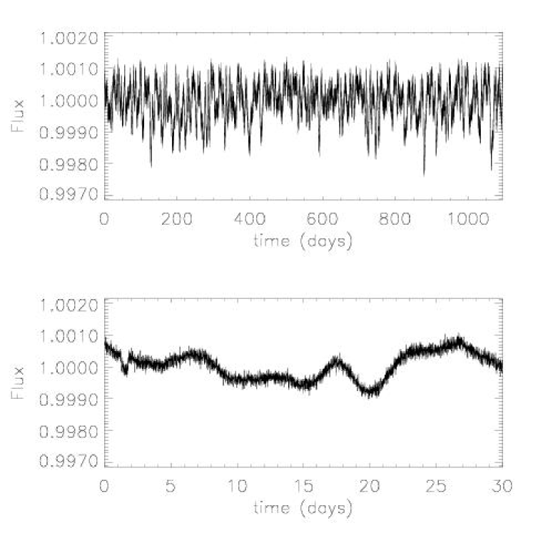
Intrinsic variability from the planet host star is expected to be the dominant noise source for space-based planetary transit searches, and for ground-based searches in the case of active stars. As an example, we use throughout the present section a light curve simulated according to the planned characteristics of the Eddington mission, containing stellar variability, planetary transits and photon noise. The procedure used to generate this light curve is described in more detail in Appendix A. The light curve, shown in Fig. 3, corresponds to a solar-age G2V star with apparent magnitude $V=13$, containing transits of a $2~{}R_{\oplus}$ planet which last $\sim 13$ hr and have a period of 1 yr. It has a sampling of 10 min and a duration of 3 yr.

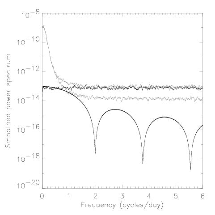
Intrinsic stellar variability can seriously impede the detection of terrestrial planets by missions such as Eddington and Kepler. However, it is possible to disentangle the planetary transit signal from other types of temporal variability if the two have sufficiently different temporal characteristics. To illustrate this we show the power spectra of the different components contributing to the light curve mentioned above in Fig. 4. Although the power contained in the transit signal is small compared to both stellar and photon noise components (and would be even smaller for the case of an Earth-size planet), it retains significant power for frequencies higher than $\sim 1~{}\mu$Hz, where the stellar signal starts to drop off steeply. As long as this condition is fulfilled (i.e. if the stellar variability occurs on sufficiently long timescales), one should be able to separate and detect the transits. Furthermore, in the case of multiple transits, the regular period of the transits also helps constrain the Fourier space occupancy of the transit signal with respect to the stellar signal.

3.1 Wiener or matched filtering approach

Carpano et al. (2003) demonstrated how use of an optimal filter can simultaneously pre-whiten and enhance the visibility of transits in data dominated by stellar variability. The Fourier-based method presented there is also closely related to a minimum mean square error (MMSE) Weiner filter. However, even for space-based missions uneven sampling of the data will occur. In these real-life cases, irregularly sampled data implies that standard Fourier methods are no longer directly applicable and a more general technique is required.

Figure 4: Power spectrum of the light curve shown in Fig. 3 (upper grey line). Lower grey line: stellar variability only. Lower black line: transits only (3 transits). Upper black line: photon noise. The power spectrum is dominated by stellar variability at low frequencies and by photon noise at high frequencies.

To gain some insight to the problem consider the general case of intrinsic stellar variability, with the received signal $x(t)$ is composed of the three components:

$$x(t)=s(t)+r(t)+n(t)$$ (19)

where $s(t)$ is the intrinsic time variable stellar light curve, $r(t)$ is the transiting planet signal, and $n(t)$ denotes the measurement plus photon noise, which we can take to be random (and Gaussian in the cases of interest here). Each component is statistically independent, hence the expected power spectrum $\Phi(\omega)$ of the received signal is simply given by:

$$\Phi(\omega)=\left<|S(\omega)|^{2}\right>+\left<|R(\omega)|^{2}\right>+\left<|N(\omega)|^{2}\right>$$ (20)

and in the case of random, or white, noise $\left<|N(\omega)|^{2}\right>$ is a constant, hence guaranteeing positivity of the right hand term. This also highlights in a natural way a justification for the somewhat arbitrary constant in Eq. (6) in Carpano et al. (2003) and how its value is related to the expected noise properties (although it would be more natural to implement it as a lower bound). However, as outlined below there is a simpler way to implement their technique without the need for the additional constant.

Figure 5: Top panel: Wiener filter constructed using the light curve shown in Fig. 3 and a reference box-shaped transit of duration 0.65 d . Middle panel: Filtered light curve. Bottom panel: Idem, $1^{\rm st}$ 30 days, with a transit 1.5 d after the start.

A standard MMSE Wiener filter attempts to maximise the signal-to-noise in the component of interest, in this case $r(t)$, by convolving the data with a filter, $h(t)$, constructed from the ratio of the cross-spectral energy densities between observation and target, such that:

$$x^{\prime}(t)=h(t)\otimes x(t)\hskip 42.67912ptX^{\prime}(\omega)=H(\omega)\ X(\omega)$$ (21)

and (using ^∗ to denote complex conjugate):

$$H(\omega)=\frac{\left<R(\omega)X(\omega)^{*}\right>}{\left<X(\omega)X(\omega)^{*}\right>}=\frac{\left<|R(\omega)|^{2}\right>}{\left<|X(\omega)|^{2}\right>}$$ (22)

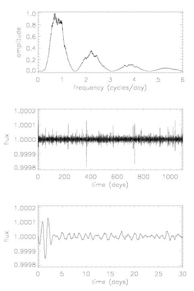
for a long enough run (a fair sample) of observations. In practice the only example we have of $x(t)$ is often singular, implying that the best estimate of the denominator is simply the observed power spectrum $\Phi(\omega)$, subject to the constraint of positivity imposed by the implicit $\left<|N(\omega)|^{2}\right>$ term. Such a filter is illustrated in Fig. 5: the top panel shows the filter, constructed using the Fourier transform of the light curve shown in Fig. 3 and a box-shaped reference transit of duration $0.65$ d, and the bottom two panels show the filtered light curve.

Figure 6: Top panel: Matched filter constructed using the light curve shown in Fig. 3 and a reference box-shaped transit of duration 0.65 d. Middle panel: Filtered light curve. Bottom panel: Idem, $1^{\rm st}$ 30 days, with a transit 1.5 d after the start.

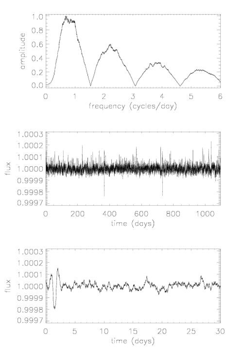
This should be contrasted with the pre-whitened matched detection filter employed by Carpano et al. (2003), illustrated in Fig. 6 (using the same layout as Fig. 5), and which can be written in the form:

$$X^{\prime}(\omega)=H(\omega)\ X(\omega)=\frac{X(\omega)}{\left<|X(\omega)|\right>}\ \left<|R(\omega)|\right>$$ (23)

and hence is equivalent to reconstructing the data using just the phase of the input signal Fourier transform modulated by the amplitude spectrum from the expected transit shape (see Fig. 7). Viewing the problem in this way removes the need for the additional constant in their Eq. (6) and emphasises the two stage nature of the filtering. The pre-whitening suppresses the stellar variability component, while the matched filter is directly equivalent to the $n=1$ ML case presented in Sect. 2.

Figure 7: As Fig. 6, but the filtered light curve was obtained by modulating the phase of the Fourier transform of the data by the amplitude spectrum of the reference transit signal. The filter was omitted as it is effectively identical to that shown in Fig. 6. Comparing, visually, the amplitude, shape and timescale of the variations in the filtered data with the bottom two panels of Fig. 6 confirms that this gives very similar results to the matched filter approach.

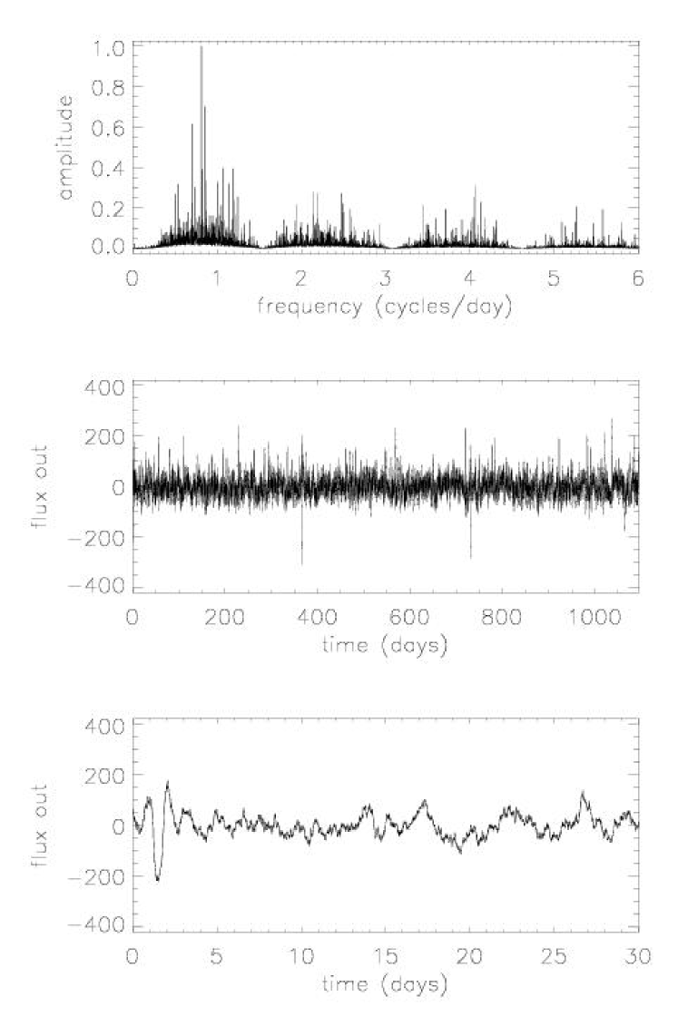
In practice, transit searching can be based directly on the output of the filtering, or preprocessing can be used to decouple the stellar variation estimation from the transit search phase, which then proceeds using the methods outlined in Sect. 2, since the problem has been reduced to the simpler one of transit detection in random noise. (In either case, detailed investigation of the transit depth and shape involves phase folding, unfiltered data, and local modelling.)

Either of these preprocessing filters works well in the case of regularly sampled data with no gaps and with a reasonable separation between the signatures of the Fourier components of the transits and the stellar variability. In Figs. 5, 6 & 7, the transits are distinctly visible in the filtered light curve. The results in terms of transit detection performance using either method are very similar. For simplicity, the matched filter approach, rather than the Wiener filter, is used in the remainder of this paper.

Figure 8: Simulated light curve with data gaps. Four arbitrarily chosen sections were removed from the light curve shown in Fig. 3. Note that for this test the gaps were chosen to avoid the transit regions for comparison purposes.

Figure 9: Results of applying the matched filter independently to the 5 unbroken intervals of the light curve shown in Fig. 8. Top panel: entire filtered light curve. Middle panel: $1^{\rm st}$ 30 days. Bottom panel: another 30 d section centred on the second transit (at 366.5 d). See text for an explanation.

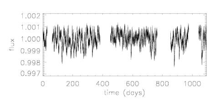
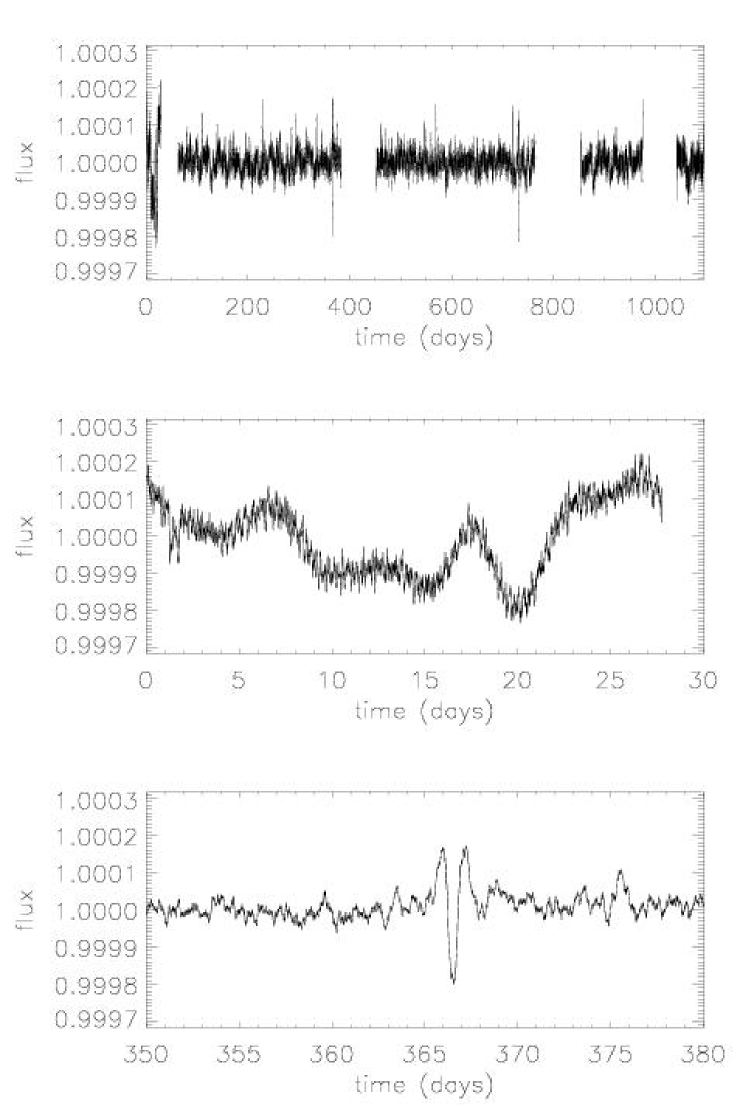
However, real data, even space-based, suffers from irregular sampling and the presence of significant gaps. Fourier domain methods cannot be directly applied to irregularly sampled data, but it is possible to treat regularly sampled data with gaps as a series of $n$ independent time series, and to filter them separately. To test this, four arbitrarily chosen sections were removed from the light curve shown in Fig. 3 (see Fig. 8). The matched filter was then applied to the five unbroken intervals separately, and the results are shown in Fig. 9. Though the filtering is effective on relatively long sections of data (bottom panel) it is not successful for short intervals (middle panel), even if they are significantly longer than the transit duration. This is because the power spectrum of the stellar noise is estimated from the data in order to construct the filter. For this to be successful, the data segment needs to be at least twice as long as the longest significant timescale in the star’s variability, which is either the rotation period or the long end of the starspot lifetime distribution (Aigrain et al., 2004). In the case of the G2V star used in the simulations, the minimum data segment length for which the filtering was successful was $\sim 60$ days (last data segment in Fig. 9), consistent with a rotation period of $\sim 30$ days for such a star.

It is therefore necessary to find other means of coping with this additional complexity. We have investigated two alternative approaches: one based on a least-squares generalisation of the Fourier filtering approach; the other based on a general purpose iterative clipped non-linear filter. In both cases we use the preprocessing to attempt to remove the stellar signature, as much as possible, prior to invoking the transit detection methods developed in Sect. 2.

3.2 Least-squares filtering

For a long run of regularly sampled data, a discrete Fourier transform asymptotically approaches a least-squares fit of individual sine and cosine components (see e.g. Bretthorst 1988). This naturally suggests an extension of the approach described in Sect. 3.1 to the case of irregularly sampled data. An analogous situation occurs in the generalisation of the periodogram method to Fourier estimation of periodicity; using generic least-squares sine curve fitting is a more flexible alternative (Brault & White, 1971). This allows the case of gaps in the data, or more generally irregular sampling, to be dealt with in a consistent and simple manner.

Figure 10: Top panel: “Power spectrum” (i.e. coefficients $a_{k}$ versus frequency) obtained by the least-squares fitting method for the light curve shown in Fig. 3. Middle panel: Reconstructed light curve, obtained by summing over the fitted sine-curves up to a frequency of $\sim 1.8$ cycles/day. Bottom panel: $1^{\rm st}$ 30 days of the reconstructed light curve.

The procedure is basically identical to that employed for the Wiener filter described in the previous section, but the calculation of the Fourier transform, or power spectrum, of the received signal is replaced by an orthogonal decomposition of this signal into sine components whose amplitude, phase and zero-point are fitted by least-squares. Each of the components has the form:

$$\psi_{k}(t)=a_{k}\sin\left(2\pi kt/T+\phi_{k}\right)$$ (24)

where $T$ is the time range spanned by the data. The number of components to fit can be chosen such than the maximum frequency fitted is equal to some fraction of the Nyquist frequency, but for this one must define an equivalent sampling time $\delta t$. In the case of regular sampling with gaps, $\delta t$ is simply the time sampling outside the gaps. In the case of irregularly sampled data the definition of $\delta t$ is more open ended. However, provided that the sampling is close to regular, a good approximation will be the average time step between consecutive data points – keeping in mind that any significant gaps should be excluded from the calculation of this average. The potentially highest frequency component should then have frequency $\approx 1/\left(2\delta t\right)$, although in practice a much lower frequency cutoff for the components is all that is required.

Note that the first (zero-frequency) component is effectively the mean data value $\left<x(t)\right>$ (which can be pre-estimated and removed in a robust way e.g. by taking a clipped median). The presence of gaps in the data provides us with a natural way of obtaining several independent estimates of $\left<X_{\rm ls}(w)\right>$ by measuring it separately in each interval between gaps, or alternatively provides a natural boundary for doing independent light curve decompositions.

Figure 11: Top panel: Equivalent matched filter constructed using the light curve shown in Fig. 3 and a reference box-shaped transit of duration 0.65 d. Middle panel: Filtered light curve. Bottom panel: Filtered light curve, $1^{\rm st}$ 30 days, with a transit 1.5 d after the start.

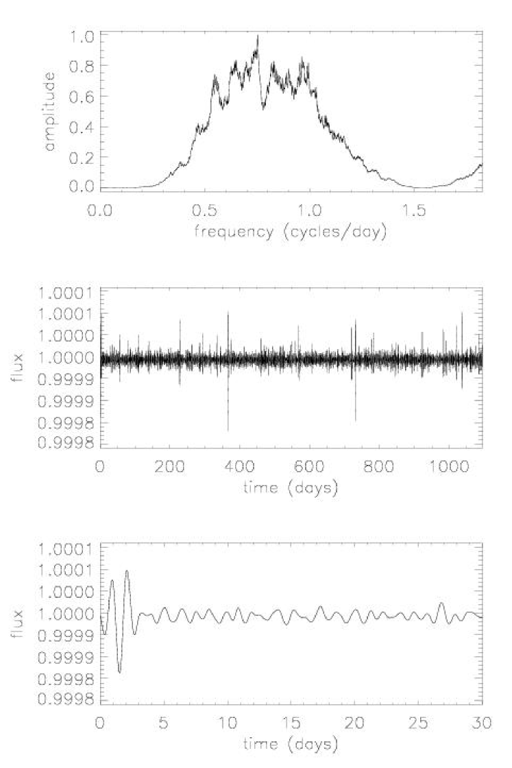
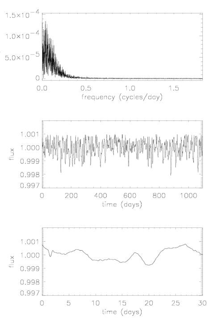
Fig. 10 illustrates this least-squares fitting method, as applied to the light curve shown in Fig. 3. The top panel shows “power spectrum”, i.e. the coefficients $a_{k}$ versus frequency, while the bottom two panels show the light curve reconstructed by summing the fitted sine-curves. Note that high frequency variations are not reconstructed as only the first 2000 sine components were fitted (well below the Nyquist limit, but amply sufficient for the purposes of following the long timescale stellar variability).

The decomposition of the reference (transit) signal can usually be well approximated analytically. For example if a simple box-shaped transit of duration $d$ is adopted as reference signal, the $k^{\rm th}$ coefficient is given by:

$$r_{k}=\frac{\sin\left(\pi kd/\delta t\right)}{\pi kd/\delta t}$$ (25)

However, this decomposition can also be performed in the same way as for the received data, for a reference signal of any given shape. The sets of coefficients $a_{k}$ and $r_{k}$ then define the filter $h_{k}$, which is equivalent to the Wiener, or matched filter of the previous section:

$$h_{k}=\frac{\left<|r_{k}|^{2}\right>}{\left<|a_{k}|^{2}\right>}\hskip 42.67912pth_{k}=\frac{\left<|r_{k}|\right>}{\left<|a_{k}|\right>}$$ (26)

where the first expression corresponds to the standard Wiener filter, and the second to the filter used in Carpano et al. (2003).

Fig.11 illustrates this filtering method. Using the second expression in Eq. (26), a “matched filter” $h_{k}$ (top panel) is constructed from the coefficients $a_{k}$ and $r_{k}$ (the latter computed according to Eq. 25). The filtered light curve, obtained by multiplying the $a_{k}$ by $h_{k}$ and reversing the “transform”, is shown in the middle panel, with a zoom on the first 30 days in the bottom panel.

Figure 12: As Fig. 11, but the input light curve is that shown in Fig. 8, with 4 significant data gaps.

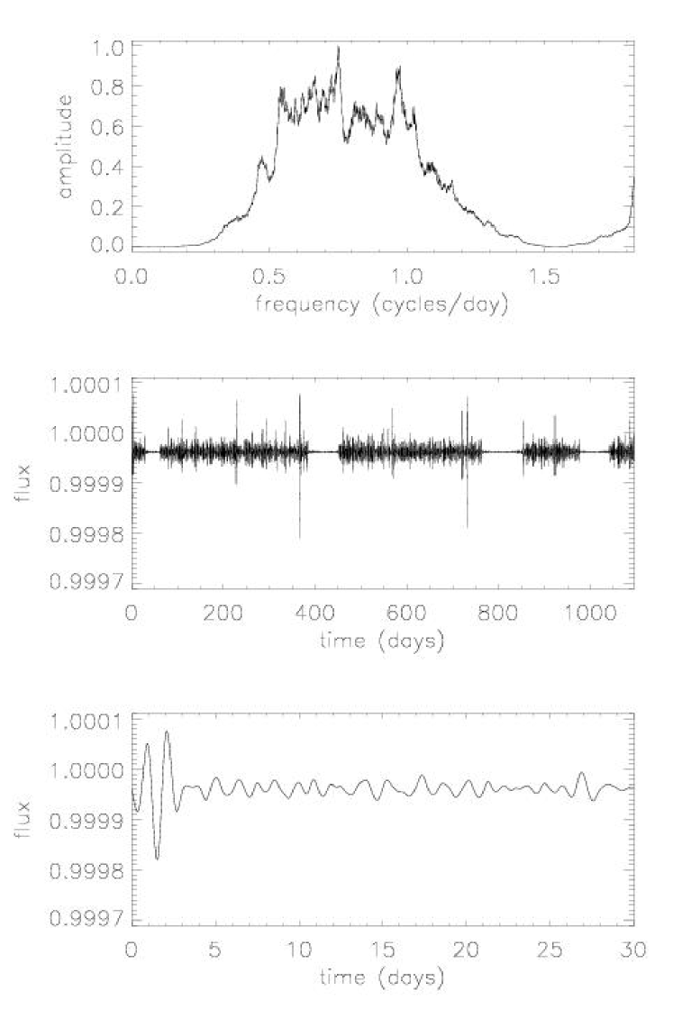
Fig. 12 shows the results of the matched filter constructed using the least-squares fitting method when the light curve contains gaps (as in Fig. 8). The performance of the filter is generally not affected by the gaps, though artifacts near gap boundaries can sometimes be introduced.

The case of irregular sampling is not illustrated here, for practical reasons: if the sampling was allowed to vary, say, by $\pm 10$ % of the normal sampling time in a random fashion, the effect is not visible in plots of such long light curves. In any case, we have found it to have negligible effect on the the least-squares filtering.

3.3 Non-linear filtering

If the timescale of the transits is shorter than the timescale for the majority of the dominant stellar variations, iterative non-linear time domain filters provide a powerful way of separating out short timescale events. A good example of this type of approach can be based around a standard median filter.

Figure 13: Light curve with data gaps filtered using the non-linear technique (black curve). The input data was the light curve shown in Fig. 8. The window of the iterative median filter used was $3\times 0.65$ d. The grey curve shows the same data with the residual noise level after filtering measured and artificial data with Gaussian distributed noise of the same standard deviation generated to fill the gaps. This illustrates the fact that, after non-linear filtering, the light curve (outside the transits) is well approximated by a constant level plus white noise.

The data is first, if necessary, split into segments, using any significant gaps in temporal coverage to define the split points. These gaps, defined as missing or bad data points, or instances where two observations are separated in time by more than a certain duration, can be automatically detected.

Each segment of data is then iteratively filtered using a median filter of window $\sim 2$ to $3$ times the transit duration, followed by a (small window) box-car filter to suppress level quantisation. The difference between the filtered signal and the original is used to compute the (robust) MAD-estimated scatter (sigma) of the residuals. The original data segments are then $k$-sigma clipped (with $k=3$) and the filtering repeated, with small gaps and subsequent clipped values flagged and ignored during the median filtering operation. The procedure converges after only a few iterations.

Break points and/or edges are dealt with using the standard technique of edge reflection to artificially construct temporary data extensions. This enables filtering to proceed out to the edges of all the data windows.

The main advantage of using a non-linear filter is that the exact shape of the transit is irrelevant and the only free parameter is the typical scale size of the duration of the transit events. The main drawback is that the temporal information in the segments is essentially ignored. However, providing the sampling within segments is not grossly irregular this has little impact in practice. This filter is also relatively fast due to its simplicity: with the same computer as before, the running time for a transit duration of $\sim 0.5$ day is 4 s per light curve, about the same as the time required for the Wiener filter. The least-squares fitting method was significantly slower (requiring approximately 30 s when 1500 frequencies were fitted).

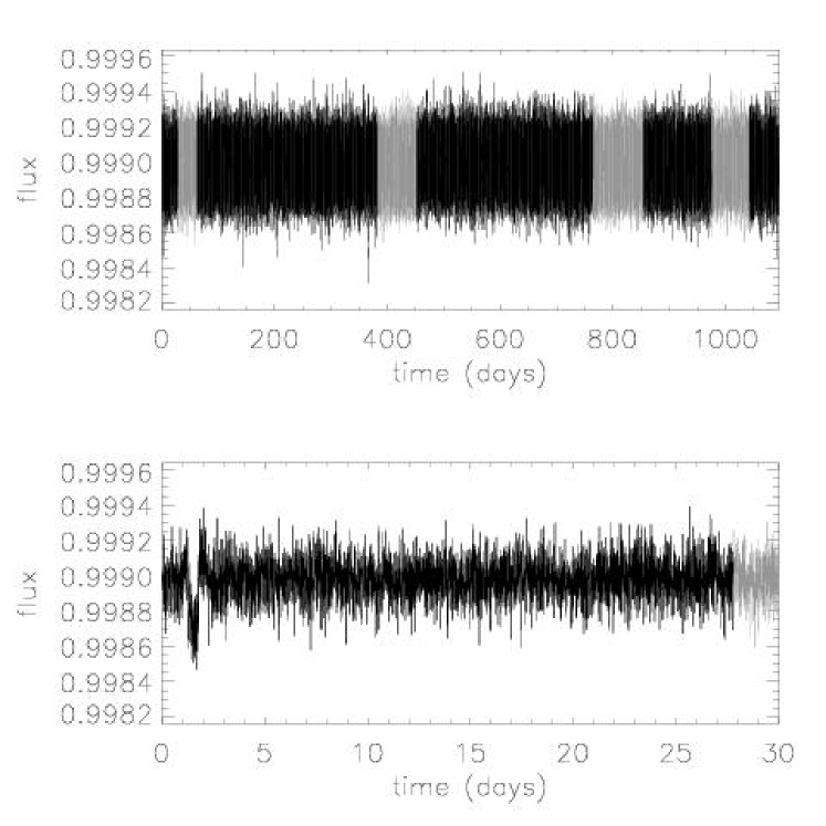
Figure 13 illustrates this method as applied to the light curve with gaps shown in Fig. 8. As with the indirect least-squares filtering, the high frequency noise remains, but this does not impede transit detection. Given the simplicity of this method and its good performance in the presence of data gaps, it appears to be the most promising, as long as the sampling remains relatively regular (if the sampling is significantly irregular, the least-squares fitting method, which takes the time of each observation into account directly, is likely to perform better).

The results of applying the transit search algorithm to the filtered light curve are shown in Fig. 14. The detection is unambiguous (and remains so for a 1.5 $R_{\oplus}$ planet with otherwise identical parameters, though the detection is not successful for a 1 $R_{\odot}$ planet with only 3 transits.

Figure 14: Results of transit search after non-linear filtering. The input of the transit search program was the black curve shown in Fig. 13. Top panel: detection statistic as a function of trial epoch for the preliminary single transit search (see Sect. 2.9). The signature of all three transits ($e=1.5$, $366.5$ & $731.5$ d) is clearly visible. Middle panel: multiple transit detection statistic as a function of trial period. Bottom panel: multiple transit detection statistic as a function of epoch at the optimal period of $365.0$ d. The detected epoch ($1.5$ d) is correct. The x-axis for the top and bottom panels were shifted by $100$ d for clarity.

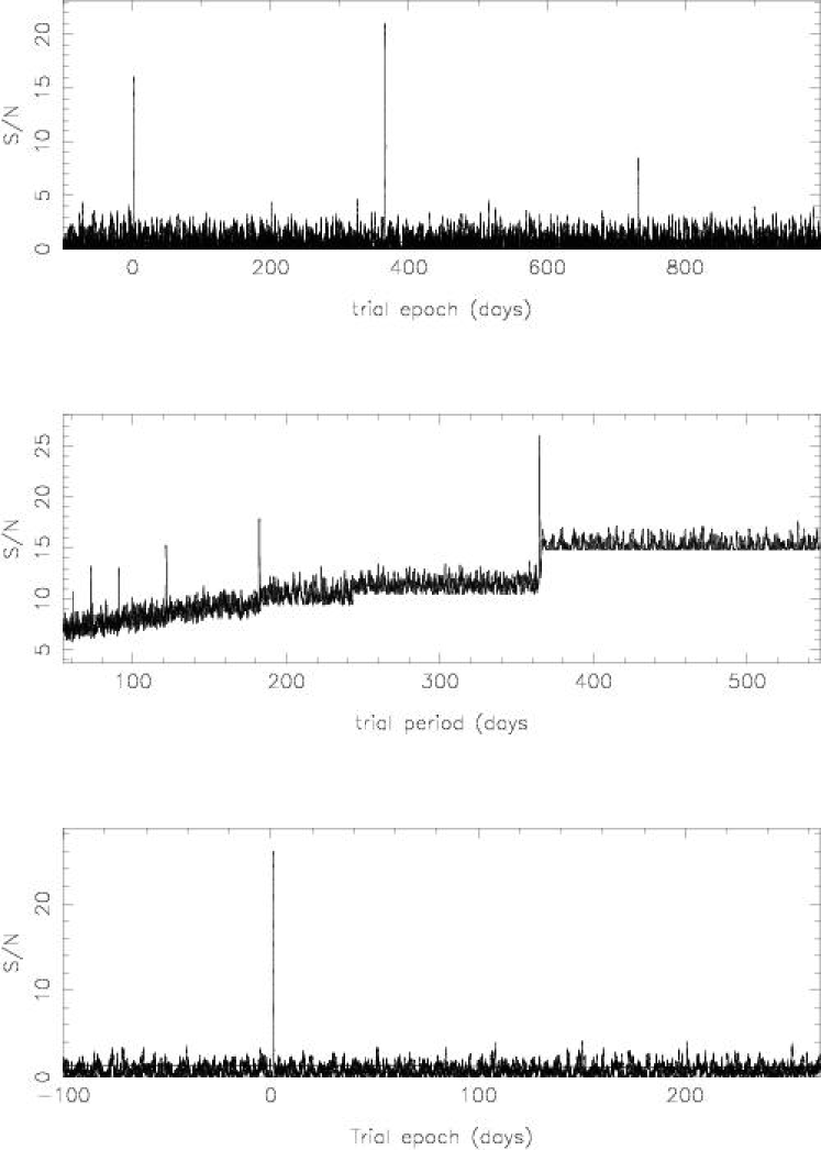
The step-like appearance and systematic slope of the middle panel (period determination) is due to a combination of the discrete (and small) number of potential transits of the phase estimation stage which precedes it and the search for a minimum (over phase) at each trial period. For each trial period the number of independent attempts to find a maximum in phase/epoch increases as the trial period increases. Furthermore, the single transit phase has negative-going excursions clipped out to enhance the detectability of real transits. This leads to a systematic bias toward higher maxima as a function of trial period. The steps are at harmonics and sub-harmonics of the fundamental period and are due to quantisation of the number of possible transits within each local trial period search.

The overall signal-to-noise ratio of the three combined transits in the filtered light curves were approximately 26, 12 and 6 for planets of radius 2.0, 1.5 and 1.0 $R_{\oplus}$ respectively. The fact that the 1.0 $R_{\oplus}$ case was not detected is therefore roughly consistent with the SNR limit of 6 stated by Kovács et al. (2002).

4 Performance evaluation

In this section, we describe Monte Carlo simulations carried out to evaluate the performance of the transit detection algorithm described in Sect. 2.5, combined with the iterative non-linear filter introduced in Sect. 3.3.

4.1 Method

The method employed was identical to that described in Section 5.1 of Aigrain & Favata (2002), which was first used in the context of transit searches by Doyle et al. (2000). The detection statistic (in this case the signal-to-noise ratio of the best candidate transit) is computed for $N$ light curves with transits. All light curves have the same parameters, but different realisations of the noise and different epochs randomly drawn from a uniform distribution (the epoch should not affect the detection process). The process is repeated for $N$ transit-less light curves, which have noise characteristics identical to those of the light curves with transits. The chosen value of 100 for $N$ is a compromise between accuracy and time constraints, and suffices to give a reasonable estimate of the performance of the method.

As the aim was to test the combined filtering and detection process, the light curves were subjected to the iterative nonlinear filter, before being forwarded to the transit detection algorithm. To avoid prohibitively time-consuming simulations, and thus to allow several star/planet configurations to be tested, a single transit duration value was used (corresponding roughly to the FWHM of the input transits).

Once the algorithm has been run on all the light curves, the next step consists in choosing a detection threshold: any light curve for which the maximum detection statistic exceeds this threshold will be considered to contain a candidate transit. If a transit-less light curve gives rise to a statistic above the threshold, a false positive: a candidate transit appears to have been detected when there is in fact none. Conversely, if the maximum detection statistic for a light curve with transits lies below the threshold, the transit(s) will go undetected: a false negative.

The optimal threshold, given a set of light curves which are known to share the same noise characteristics, can be chosen from the results of the transit search itself to minimise the false alarms and missed transits. This is illustrated in a schematic way in Figure 3 of Aigrain & Favata (2002). Detection statistic histograms ideally should show a clear separation between real transits and false alarms, allowing a simple choice of boundary between the respective distributions. The location of the boundary is chosen as a compromise between maximising the detection rate and minimising the number of false alarms.

In certain circumstances, it might be more important to minimise missed detections (for example if the sought-after events are very rare, particularly if false alarms can easily be weeded out at a later stage). In other circumstances (for example if it is very difficult to test the reliability of any candidate events through further observations) it may be more desirable to minimise false alarms. However, as our present aim is simply to carry out a simple performance evaluation, we did not give priority to either kind of error over the other and just minimised the sum of the two types of error.

4.2 Results

Figure 15: Results of the performance evaluation for 5 star/planet configurations, as detailed in Table 1. Solid histograms: distributions of the maxima of S/N statistics computed by the transit detection algorithm after non-linear filtering for 100 light curves containing transits. Dashed histograms: idem for 100 light curves containing stellar variability and photon noise only. Thick vertical lines: optimal detection threshold.

4.2.1 Photon-noise only case

The aim of this simulation was to compare the performance of the present algorithm to others, which have mostly been tested on white-noise only light curves.

If the present method is to improve on the performance of the Bayesian approach it is derived from, it should be able to detect reliably a $1.0~{}R_{\oplus}$ planet orbiting a G2V star with photon noise corresponding to $V=13$, given three transits in the light curve. In Aigrain & Favata (2002), simulations showed that such a planet should be easily detected around a smaller (K5V) but fainter ($V=14$) star with the older algorithm and no filtering. The $V=13$, G2 case corresponds to a $S/N$ that is larger by a factor of 1.07, and should therefore be detected easily if the new method is as efficient as the old.

Table 1: Light curve characteristics for each panel of Fig. 15.

Panel	a)	b)	c)	d)	e)
Photon noise	$\surd$	$\surd$	$\surd$	$\surd$	$\surd$
Stellar	$\times$	$\surd$	$\surd$	$\surd$	$\surd$
variability
Age (Gyr)	4.5	4.5	4.5	4.5	4.5
SpT	G2V	G2V	G2V	G2V	G2V
$R_{\rm pl}$ ($R_{\oplus}$)	1.0	1.0	1.5	1.0	1.0
Period (yr)	1.0	1.0	1.0	0.5	1.0

After a set of simulations was run for such a configuration, the maximum detection statistic from the noise only light curves was $S/N=5.79$, while the minimum value from the light curves with transits was $S/N=7.41$ (see Fig. 15a). Any threshold in between would therefore allow the detection of all the transits where present, with no false alarms.

Note that the $S/N$ limit of 6, quoted by Kovács et al. (2002) for their BLS method, which is statistically close to ours, falls as expected in the range of thresholds that would be suitable in the present case.

4.2.2 Photon noise and stellar variability

$\bullet$ $1.0~{}R_{\oplus}$ planet orbiting a G2V star
This configuration is identical to that in Sect. 4.2.1, but with stellar variability added. It is also similar to the case illustrated in Figs. 3 to 14, but with a smaller planet. The results are shown in Fig. 15b. The distributions of the detection statistics from the light curves with and without transits overlap almost entirely, i.e. the performance is poor. The threshold that minimises the sum of false alarms and missed detection leads to 56 of the first and 26 of the second.

Assuming that the sampling rate, light curve duration, and stellar apparent magnitude are fixed, there are three factors which should lead to better performance: a larger planet, a shorter orbital period (i.e. more transits) or a smaller star. Each of these options in turn is investigated below.

$\bullet$ $1.5~{}R_{\oplus}$ planet orbiting a G2V star
The histograms are relatively well separated (see Fig. 15c), with only a small overlap, so that the optimal threshold of $S/N=7.85$ lead to one missed detection and no false alarms.

It is interesting to note the similarity between the results of this simulation and the requirements used for the design of the Kepler mission, which was to detect planets given a signal-to-noise ratio totalling at least 8 for at least three transits.

$\bullet$ $1.0~{}R_{\oplus}$ planet orbiting a G2V star with 6 transits
The aim of this set of simulations was to investigate the effect of increasing the number of transits in the light curve by a factor of two by reducing the orbital period to 182 d. This is equivalent to increasing the overall duration of the observations. As expected, this leads to higher $S/N$ values and hence better performance, with only 13 false alarms and 16 missed detections (see Fig. 15d).

$\bullet$ $1.0~{}R_{\oplus}$ planet orbiting a K5V star
A K5 star is smaller than a G2 star, leading to deeper transits, but also more active, leading to more stellar variability. Recent studies(Aigrain et al., 2004) suggested that the former effect prevailed over the latter, and that K or even M type stars might make better targets for space missions seeking to detect habitable planets than G stars, but these were based only on results from a few individual light curves, rather than Monte Carlo simulations.

The present tests confirm this trend: the separation between the with- and without transit distributions is wider (see Fig. 15e) than in the previous case, though the best-threshold false alarm and missed detection rates remain high at 13 and 25 % respectively.

Note the higher $S/N$ values for the transit-less light curves compared to the G2 case, which suggests the presence of more residual stellar variability after filtering, as would be expected.

5 Discussion

Starting from a general purpose maximum likelihood approach we have demonstrated the the links between a variety of period and transit finding methods and have shown that matched filters, cross-correlation, least-squares fitting and maximum likelihood methods are all facets of the same underlying principle. In the simple approximation of rectangular-shaped transits embedded on a flat continuum and in white noise, all of these approaches can be tuned to give similar detection results.

The transit detection algorithm presented here provides a unified approach linking all these methods. Computational efficiency is of particular importance in the context of large, long duration, high sampling missions such as Eddington and Kepler, and the present method would allow a search for transits by habitable planets to be performed on 20,000 3 yr long light curves with 10 min sampling in less than a day. Including the time required to apply the nonlinear filter, which for the laptop used takes $\sim 4\,$s per light curve per filter duration, this would increase to $\sim 3\,$d (using three different filter durations). This is achieved at no cost in efficiency: in white noise only, the algorithm is capable of detecting transits down to approximately the same $S/N$ limit as that quoted by Kovács et al. (2002) for their BLS method, which has been the most successful method to date in terms of practical results, being used by the OGLE team to discover most of their candidate transits, see (Udalski et al., 002b, 2003).

This approach is predicated on the assumption of periodic transits hidden in random noise, usually assumed to be superposed on a flat continuum with regular continuous sampling. In the real world, stellar (micro) variability is expected to be the dominant signal component. We have then shown how to generalise the transit finding method to the more realistic scenario where complex stellar variability, irregular sampling and long gaps in the data, are all present.

The two filtering methods developed to deal with this case share some advantages – both can be applied to data with gaps – but they also have different properties. The least-squares fitting method is capable of making use of the time information in data with irregular sampling. It also allows a theoretically optimal filter (i.e. the Wiener or matched filter) to be combined with a pre-whitening filter, although from the point of view of detection, the matched filter is the main active component of any maximum likelihood-based detection algorithm. As a by product of the filtering, the stellar signal can also be reconstructed. However, this is computationally intensive, particularly if one wishes to fit higher frequencies. Its performance also depends quite critically on concordance between the duration of the reference transit and that of any true transit.

On the other hand, iterative non-linear filtering is simple to implement and fast, but ignores any local time information (except for the long gaps which are detected automatically). This means that its performance is likely to degrade if the sampling is seriously irregular. However, it is the most efficient method in cases such as those investigated here. By removing any signal on timescales longer than two-three times the estimated transit duration, it is likely to be less affected by the value chosen for that duration. Although more work is needed to establish quantitatively the relative merits of the two approaches, it seems more efficient, given the results so far, to use the iterative non-linear filtering method prior to a general transit search. The least-squares fitting method could be employed in the more difficult (e.g. very irregular sampling) or borderline (as in Sect. 4.2.2) cases, where the additional information used about the transit shape may lead to better performance.

Whatever the method used, there is a fundamental limit to what can be achieved. Stellar variability can only be filtered out if an orthogonal decomposition of the transit and stellar signal is possible, e.g. if the two signatures in the frequency domain do not overlap by too much. Therefore, very rapidly rotating stars where the rotation period is close to the transit duration, or stars showing much more power than the Sun on timescales of minutes to hours (e.g. higher meso- or super-granulation) will be problematic targets. Even in the hypothetical situation where all stellar noise is removed, the remaining white noise will also place a limit on the performance of the transit detection algorithm, and hence on the apparent magnitude of star around which transits of a certain depth can be found. In white Gaussian noise, any transit yielding a signal-to-noise ratio above a fixed threshold (estimated to be $\approx 6$ in Sect. 4.2.1) should be detectable. Considering photon noise alone, for a given stellar radius, orbital period and transit duration, the smallest detectable planet radius would therefore scale as $B^{-1/4}$ or $\exp(m/10)$ where $B$ and $m$ are the star’s apparent brightness and magnitude respectively.

The natural progression of this work will be further quantification of the performances attained, and the identification of the best method to use for a given situation (i.e. star-planet combination, instrument characteristics and/or sampling). As in the present paper, this can be done through Monte Carlo simulations, and more realistic noise profiles can be included in the light curves (e.g. instrumental noise). Extensive simulations can be performed for a given target field by coupling the stellar variability model to a galactic population model and any available extinction information on the field. However, it will only be meaningful to carry out such simulations when the design, target fields and observing strategies of the missions in question are finalised and when more information about stellar micro-variability is available.

Our main conclusion if that even with realistic contamination from stellar variability, irregular sampling, and gaps in the data record, it is still possible to detect transiting planets with an efficiency close to the idealised theoretical bound. In particular, space missions are tantalisingly close to being capable of detecting earth-like planets around G and K dwarfs.

Appendix A Simulation of realistic Eddington light curves

In this appendix we briefly outline the method used to simulate the light curves shown in Figs. 3 & 8.

A.1 Planetary transits

Deeg (1999)’s IDL based Universal Transit Modeller (UTM) was used to simulate noise-free light curves. UTM includes a linear limb-darkening law, and limb-darkening coefficients from Van Hamme (1993) were used. For a given star-planet configuration, the other input parameters were the ratio of planetary to stellar radius, the planet’s orbital period and distance, and the sampling time and duration. For the latter, values of 10 min and 3 yr respectively were used, as appropriate for Eddington in planet-finding mode (Favata, 2003). The output is in units of relative flux, normalised to an out-of-transit value of 1.0. These units are used throughout. Note that no reflected light from the planet is included, and that all orbits are assumed to be circular. The planet’s orbital plane is also assumed to be aligned along the line-of-sight.

For the current paper, we chose to model a $2~{}R_{\oplus}$ planet orbiting a G2V star ($R_{\star}=1.03~{}R_{\odot}$), i.e. a radius ratio of $0.018$, leading to a relative transit depth of $3.24\times 10^{-4}$. This is not the smallest detectable planet around such a star (with the methods presented here), but it is the smallest for which transits are visible by eye in both the pre- and post-filtering light curves. The planet’s orbital period is 1 yr, and its orbital distance 1 AU. The epoch of the first transit is 1.5 d. The power spectrum of this transit-only light curve is shown as the black line with repeated “humps” in Fig. 4.

A.2 Intrinsic stellar variability

The model used to simulate stellar micro-variability, which allows the generation of light curves for stars of various spectral types and ages, was presented in detail in Aigrain et al. (2004), with the aim of testing and refining filtering and transit detection algorithms, in the context of space-based transit searches such as COROT, Eddington and Kepler.

The starting point for the model is the Sun’s photometric variability, which has been studied at ultra-high precision since January 1996 by the VIRGO experiment (Frohlich et al., 1997) onboard the SoHO observatory. Empirical scaling laws, either published (Skumanich, 1972; Noyes et al., 1984) or derived from published datasets (Radick et al. 1987; Radick et al. 1995; Radick et al. 1998; Henry et al. 2000, for a wide range of stars), are then used to scale the amplitude and frequency distribution of the Sun’s variability to other stellar ages and masses.

Light curves can be generated for dwarfs of any spectral type between F5 and K5, and for all ages later than the Hyades (625 Myr, Perryman et al. 1998). In the present paper, a 4.5 Gyr old G2V star was modelled, again with a sampling time of 10 min and duration of 3 yr. The stellar light curve, also in relative flux units (and whose power spectrum is shown as the lower grey line in Fig. 4), is then multiplied by the planetary light curve described in A.1.

The IDL source code used to construct these, together with a number of existing simulated light curves, are available from www.ast.cam.ac.uk/~suz/simlc.

A.3 Photon noise

The Eddington baseline configuration, at the time of writing, consists of four co-aligned wide-field telescopes, with a total collecting area of $0.764~{}{\rm m}^{2}$. Combined with the optics and CCD performance, this leads to an expected photon count of, for example, $1.4\times 10^{5}~{}\gamma~{}{\rm s}^{-1}$ for a $V=13$ star. The photon noise in relative flux units should thus be well approximated by a Gaussian distribution with a normalised standard deviation of $1.09\times 10^{-4}$ for 10 min integrations, and such a randomly generated photon noise value was added to each data point in the combined star-planet light curve. The result is the light curve shown in Fig. 3, while the power spectrum of the noise component is shown as the approximately constant black line in Fig. 4.

A.4 The above with gaps

To investigate the impact of data gaps, the following four sections of data were removed from the gap-less light curve:

• indices 4 000 to 8 999 (i.e. $t=27.8$ to 62.5 d);

• indices 55 092 to 65 060 (i.e. $t=382.6$ to 451.8 d);

• indices 110 000 to 123 009 (i.e. $t=763.9$ to 854.2 d);

• indices 140 395 to 149 999 (i.e. $t=975.0$ to 1041.7 d).

These were chosen arbitrarily, but with the aim of ensuring a variety of gap and data interval durations, and avoiding the removal of any transits. In reality, data gaps are of course likely to affect the number of observed transits, but this is a different issue to that investigated here, i.e. the development of filters which can remove the stellar signal in the presence of gaps regardless of the presence (or lack) of transits. The resulting light curve is shown in Fig. 8.

Note that missions like Eddington are expected to have a very high duty cycle ($>95$ % – Favata, priv. comm.), compared to a value of $\sim 70$ % for the simulated light curve used in the present work. Such a low duty cycle is therefore even more conservative than the expected worst case scenario.

References

- Aigrain & Favata (2002) Aigrain S., Favata F., 2002, A&A, 395, 625
- Aigrain et al. (2004) Aigrain S., Favata F., Gilmore G., 2004, A&A, in press
- Baglin & the COROT Team (2003) Baglin A., the COROT Team 2003, Adv. Sp. Res., p. 345
- Borucki et al. (2003) Borucki W. J., Koch D. G., Lissauer J. J., Basri G. B., Caldwell J. F., Cochran W. D., Dunham E. W., Geary J. C., Latham D. W., Gilliland R. L., Caldwell D. A., Jenkins J. M., Kondo Y., 2003, in Blades J. C., Siegmund O. H. W., eds, Future EUV/UV and Visible Space Astrophysics Missions and Instrumentation Vol. 4854 of SPIE, The Kepler mission: a wide-field-of-view photometer designed to determine the frequency of Earth-size planets around solar-like stars. pp 129–140
- Brault & White (1971) Brault J. W., White O. R., 1971, A&A, 13, 169
- Bretthorst (1988) Bretthorst G. L., 1988, Bayesian Spectrum Analysis and Parameter Estimation. Vol. 48 of Lecture Notes in Statistics, Springer-Verlag, New York
- Carpano et al. (2003) Carpano S., Aigrain S., Favata F., 2003, A&A, 401, 743
-
Deeg (1999)
Deeg H. J., , 1999,
www.iac.es.galeria/hdeeg/idl_hans_lib/utm - Defaÿ et al. (2001) Defaÿ C., Deleuil M., Barge P., 2001, A&A, 365, 330
- Doyle et al. (2000) Doyle L. R., Deeg H. J., Kozhevnikov V. P., Oetiker B., Martín E. L., Blue J. E., Rottler L., Stone R. P. S., Ninkov Z., Jenkins J. M., Schneider J., Dunham E. W., Doyle M. F., Paleologou E., 2000, ApJ, 535, 338
- Dreizler et al. (2003) Dreizler S., Hauschildt P. H., Kley W., Rauch T., Schuh S. L., Werner K., Wolff B., 2003, A&A, 402, 791
- Favata (2003) Favata F., 2003, in F. F., Aigrain S., eds, Proceedings of the second Eddington workshop on stellar structure and habitable planet finding ESA SP-538, The Eddington mission. p. in press
- Frohlich et al. (1997) Frohlich C., Andersen B., Appourchaux T., Berthomieu G., Crommelynck D. A., Domingo V., Fichot A., Finsterle W., Gomez M. F., Gough D., others 1997, So. Ph., 170, 1
- Gregory (1999) Gregory P. C., 1999, ApJ, 520, 361
- Gregory & Loredo (1992) Gregory P. C., Loredo T. J., 1992, ApJ, 398, 146
- Henry et al. (2000) Henry G. W., Baliunas S. L., Donahue R. A., Fekel F. C., Soon W., 2000, AJ, 531, 415
- Hidas et al. (2003) Hidas M. G., Ashley M. C., Webb J. K., Irwin M., Aigrain S., Toyozumi H., 2003, in IAU Symposium Vol. 219, a southern search for transiting extrasolar planets. p. 56
- Hoaglin et al. (1983) Hoaglin D. C., Mostellar F., Tukey J. W., eds, 1983, Understanding robust and exploratory data analysis. John Wiley, New York Chichester
- Horne (2002) Horne K., 2002, in F. F., Roxburgh I. W., Galadi D., eds, Proceedings of the First Eddington Workshop on Stellar Structure and Habitable Planet Finding ESA SP-485, Planetary transit surveys. pp 137–145
- Jenkins (2002) Jenkins J. M., 2002, ApJ, 575, 493
- Jenkins et al. (2002) Jenkins J. M., Caldwell D. A., Borucki W. J., 2002, ApJ, 564, 495
- Konacki et al. (2003) Konacki M., Torres G., Jha S., Sasselov D. D., 2003, Nat, 421, 507
- Kovács et al. (2002) Kovács G., Zucker S., Mazeh T., 2002, A&A, 391, 369
- Mallén-Ornelas et al. (2003) Mallén-Ornelas G., Seager S., Yee H. K. C., Minniti D., Gladders M. D., Mallén-Fullerton G. M., Brown T. M., 2003, ApJ, 582, 1123
- Mayor & Queloz (1995) Mayor M., Queloz D., 1995, Nat, 378, 355
- Noyes et al. (1984) Noyes R. W., Hartmann L. W., Baliunas S. L., Duncan D. K., Vaughan A. H., 1984, ApJ, 279, 763
- Perryman et al. (1998) Perryman M. A. C., Brown A. G. A., Lebreton Y., Gomez A., Turon C., Cayrel de Strobel G., Mermilliod J. C., Robichon N., Kovalevsky J., Crifo F., 1998, A&A, 331, 81
- Radick et al. (1998) Radick R. R., Lockwood G. W., Skiff B. A., Baliunas S. L., 1998, ApJS, 118, 239
- Radick et al. (1995) Radick R. R., Lockwood G. W., Skiff B. A., Thompson D. T., 1995, ApJ, 452, 332
- Radick et al. (1987) Radick R. R., Thompson D. T., Lockwood G. W. e. a., 1987, ApJ, 321, 459
- Skumanich (1972) Skumanich A., 1972, ApJ, 171, 565
- Street et al. (2003) Street R. A., Horne K., Lister T. A., Penny A., Tsapras Y., Quirrenbach A., Safizadeh N., Cooke J., Mitchell D., Collier Cameron A., 2003, MNRAS, 340, 1287
- Tingley (003a) Tingley B., ”2003a”, A&A, 403, 329
- Udalski et al. (002a) Udalski A., Paczynski B., Zebrun K., Szymaski M., Kubiak M., Soszynski I., Szewczyk O., Wyrzykowski L., Pietrzynski G., 2002a, Acta Astron., 52, 1
- Udalski et al. (2003) Udalski A., Pietrzynski G., Szymanski M., Kubiak M., Zebrun K., Soszynski I., Szewczyk O., Wyrzykowski L., 2003, AcA, 53, 133
- Udalski et al. (002b) Udalski A., Zebrun K., Szymanski M., Kubiak M., Soszynski I., Szewczyk O., Wyrzykowski L., Pietrzynski G., 2002b, Acta Astron., 52, 115
- Van Hamme (1993) Van Hamme W., 1993, ApJ, 106, 2096