Variations in Star Formation History and the Red Giant Branch Tip

Abstract

We examine the reliability of the tip of the red giant branch (TRGB) as a distance indicator for stellar populations with different star formation histories (SFHs) when photometric errors and completeness corrections at the TRGB are small. In general, the TRGB-distance method is insensitive to the shape of the SFH except when it produces a stellar population with a significant component undergoing the red giant branch phase transition. The I-band absolute magnitude of the TRGB for the middle and late stages of this transition ($\sim 1.3-1.7$ Gyr) is several tenths of a magnitude fainter than the canonical value of $\rm M_{I}\approx-4.0$. If more than $\sim 30\%$ of all stars formed over the lifetime of the Universe are formed at these ages, then the distance could be overestimated by $\sim 10-25\%$. Similarly, the TRGB-distance method is insensitive to the metallicity distribution of stars formed except when the average metallicity is greater than $\rm\langle[Fe/H]\rangle=-0.3$. If more than $\sim 70\%$ of all stars formed have [Fe/H] $>-0.3$, the distance could be overestimated by $\sim 10-45\%$. We find that two observable quantities, the height of the discontinuity in the luminosity function at the TRGB and the median $\rm(V-I)_{0}$ at $\rm M_{I}=-3.5$ can be used to test if the aforementioned age and metallicity conditions are met.

1 Introduction

The tip of the red giant branch (TRGB) marks the onset of helium fusion in stars. For old, low-mass stars this is an explosive event called the helium flash. During the helium flash these stars undergo a quick readjustment of their interiors before they begin helium burning on the horizontal branch. Therefore, the TRGB is manifested as a sharp discontinuity in the RGB luminosity function (LF). Theoretical models and observational data agree that the I-band absolute magnitude of the TRGB is located at $\rm M_{I}(TRGB)\approx-4.0\ \pm\ 0.1$ for metallicities in the range $-2.2\lesssim{\rm[Fe/H]}\lesssim-0.7$ and ages between 2 and 15 Gyr (Da Costa & Armandroff 1990; Lee, Freedman, & Madore 1993; Bellazzini, Ferraro, & Pancino 2001). The reason for this is twofold. First, the mass of the degenerate helium core and hence, the stellar luminosity, is approximately constant in this age range. Second, the stellar spectrum peaks near the I-band in these age and metallicity ranges making $\rm M_{I}(TRGB)$ approximately constant. Therefore, $\rm M_{I}(TRGB)$ can be used as a standard candle for measuring distances to resolved stellar populations.

Numerous studies have taken advantage of the TRGB standard candle to measure distances to galaxies in the Local Group and beyond (e.g. M$\rm\acute{e}$ndez et al. 2002; Karachentsev et al. 2002; Sakai et al. 1997; Cioni et al. 2000; Sarajedini et al. 2002; Jerjen & Rejkuba 2001; Ma$\rm\acute{i}$z-Apell$\rm\acute{a}$niz, Cieza, & MacKenty 2002; Sakai, Zaritsky, & Kennicutt 2000; Sakai, Madore, & Freedman 1999). Such distance measurments are important for calibrating other distance measurement techniques, for measuring the local velocity field (M$\rm\acute{e}$ndez et al. 2002; Karachentsev et al. 2002), and for determining accurate SFHs of the galaxy stellar populations. However, many of these studies make an assumption that the target RGB populations occupy the required age and metallicity ranges.

In this paper, we examine the effects of star formation history (SFH) variations on the TRGB-distance method. In particular, we generate synthetic color-magnitude diagrams (CMDs) for stellar populations with a range of ages and metallicities and employ standard observational techniques to determine the I magnitude of the TRGB. Since the distance to each synthetic population is known, we can quantitatively evaluate the systematic errors associated with the SFH variations on the TRGB-distance method. We define old stars as those having ages $>10$ Gyr, intermediate-age stars as those with ages between 2 and 7 Gyr, and young stars as those with ages $<2$ Gyr.

2 Methods

2.1 Synthetic color-magnitude diagrams

To generate synthetic CMDs, we use the StarFISH software introduced by Harris & Zaritsky (2001). Given an SFH, distance modulus, extinction law, reddening, initial mass function (IMF) slope and binary fraction, this code uses theoretical isochrones to generate photometry for artificial stellar populations. We adopt the Padova set of isochrones (Girardi et al. 2000) which cover metal abundances of Z = 0.0004, 0.001, 0.004, 0.008, 0.019, 0.030 and an age range of log(age/yr) = $7.80-10.25$. These isochrones include evolution from the main sequence to either the thermally pulsing asymptotic giant branch (AGB) stage or carbon ignition so all of our synthetic CMDs contain AGB stars at luminosities higher than or comparable to that of the TRGB. To increase metallicity resolution we linearly interpolate between each metallicity pair resulting in another set of isochrones with the same ages but metallicities of Z = 0.0007, 0.0025, 0.006, 0.0135, and 0.0245. For simplicity and clarity, we use a distance modulus of zero, Salpeter IMF, binary fraction of 0.25, and zero reddening.

The StarFISH software populates isochrones with stars in a realistic manner; the probability of finding a star at any point along the isochrone depends on the IMF and on the evolutionary timescale of that particular point. To reproduce observational effects, the stars added to an isochrone are probabilistically removed and scattered according to photometry-dependent completeness rate and error tables.

2.2 Photometric errors and completeness

Generating accurate synthetic CMDs requires a proper analysis of how photometric errors and completeness fraction change with magnitude and color. When studying a real stellar population, this analysis is done with artificial star tests in which stars of known magnitudes and colors are placed in the original images and the data reduction is repeated. The completeness fraction is estimated from the number of recovered artificial stars whose colors and magnitudes are then compared to the input colors and magnitudes to estimate photometric errors (e.g. Aparicio & Gallart 1995).

Because the TRGB is a relatively confined region of the CMD the photometric errors and completeness fraction do not change significantly over the region of interest. Moreover, photometric errors are typically small in this region because it is usually one of the brightest features of a CMD. Crowding also is generally not severe in nearby dwarf galaxies and in the halos of LG galaxies where the TRGB-distance method is typically applied. However, when applying the TRGB-distance method to galaxies beyond the LG or in very crowded stellar regions nearby, the errors and completeness rate can be much more important. Investigating the effect of SFH variations on the TRGB in such cases is beyond the scope of the present study.

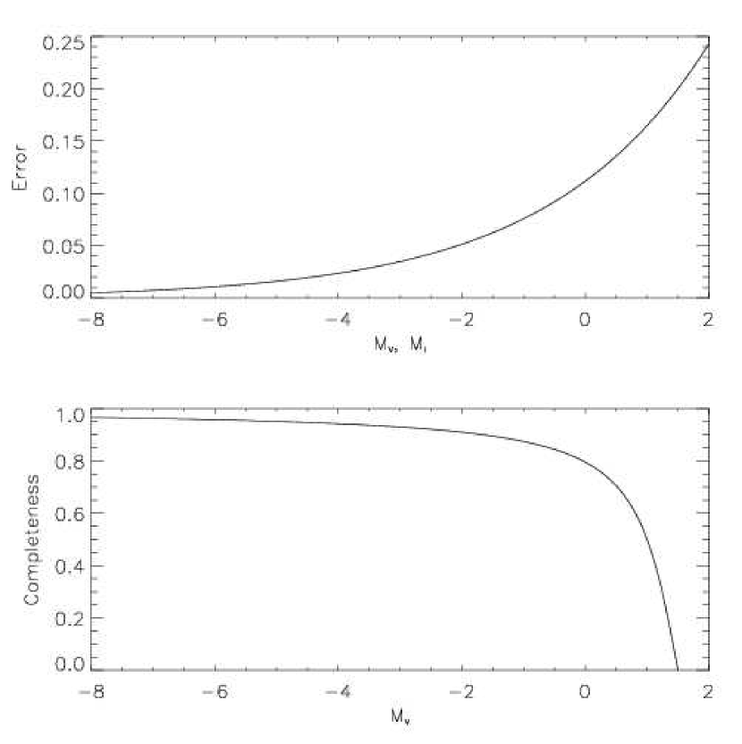
Given the previous considerations, we choose to use simple analytic functions for the photometric errors and completeness rate which are fairly typical of data taken with HST or ground-based telescopes (e.g. Aparicio & Gallart 1995; Sarajedini et al. 2002). These functions are plotted in Fig. 1 assuming the parameter values given below. Photometric errors are modeled with an exponential function of the form,

$$\sigma(M)=\kappa e^{\tau M},$$ (1)

where M is $\rm M_{I}$ or $\rm M_{V}$ and $\kappa$ and $\tau$ are constants. Given the boundary conditions $\rm\sigma(M_{I}=-8.0)=0.005$ and $\rm\sigma(M_{I}=1.5)=0.2$, these constants take the values $\kappa=0.11$ and $\tau=0.39$. Completeness is modeled with the function,

$$f(M_{V})=-\frac{2}{\pi}\arctan[\alpha(M_{V}-M_{V_{0}})],$$ (2)

where $\alpha$ is a shape parameter that affects the steepness of the fall-off and $\rm M_{V_{0}}$ is the magnitude at which the completeness equals 0%. For all our CMDs we use $\alpha$ = 2.0 and $\rm M_{V_{0}}$ = 1.5 which yield a completeness rate of 50% at $\rm M_{V}$ = 1.0.

Each star is probabilistically removed according to the completeness fraction at the star’s $\rm M_{V}$ magnitude. If a star is kept, its photometry is scattered by randomly drawing from a Gaussian distribution with standard deviation equal to its error given by Equ. 1.

2.3 Calibration of $\rm M_{I}(TRGB)$

To use the TRGB as a distance indicator it must be calibrated by using nearby stellar populations whose distances are known from other independent techniques. Several studies have done just that. Da Costa & Armandroff (1990) used the RGBs of eight Galactic globular clusters to derive the I-band bolometric correction as a function of $\rm(V-I)_{0}$ color, the bolometric magnitude of the TRGB as a function of [Fe/H], and [Fe/H] as a function of $\rm(V-I)_{0}$ color at $\rm M_{I}=-3.0$. Using a slightly revised version of the latter relation more appropriate for galaxies, Lee et al. (1993) demonstrated that the TRGB method had the precision of primary distance indicators like Cepheids and RR Lyraes. Most recently, Bellazzini et al. (2001) derived a new empirical relation between $\rm M_{I}(TRGB)$ and [Fe/H] based on the largest IR database of Galactic globular cluster RGBs and calibrated over a larger range of metallicities.

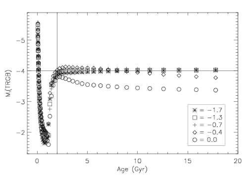
Since we are studying CMDs generated from theoretical isochrones, it is logical to use a theoretical rather than empirical calibration of the TRGB. In Fig. 2, we plot the I-band absolute magnitude of the TRGB as a function of age for different metallicities. These data are taken from the summary tables of the Padova isochrones. For ages between 2 and 15 Gyr and $\rm-1.7\leq[Fe/H]\leq-0.7$, $\rm M_{I}(TRGB)$ lies in the range $-4.0\pm 0.05$, where 0.05 is the standard deviation. We use this theoretical estimate of $\rm M_{I}(TRGB)$ as a fiducial value when analyzing our synthetic CMDs.

It is worthwhile to take a closer look at Fig. 2. The qualitative behavior of $\rm M_{I}(TRGB)$ may be completely explained by considering the results of Sweigart, Greggio, & Renzini (1990). They examined in detail the dependence of the core mass on the total stellar mass at the TRGB. They found that for stars massive enough to avoid the degenerate conditions that lead to the He flash, the core mass is approximately linearly proportional to the total mass. For low-mass stars, the core mass is completely degenerate and therefore insensitive to total mass. But for stars in between these two regimes, known as the RGB phase transition, the core mass increases quickly with decreasing total mass. Because the luminosity at the TRGB is so closely coupled to the core mass, it follows the same pattern. Since the total mass at the TRGB decreases with age, the luminosity has a similar dependence on age as it does on total mass. Finally, since $\rm M_{I}$ is proportional to luminosity, except when the metal abundance is high enough that line-blanketing becomes significant in the I-band, $\rm M_{I}$ should depend on age the same way luminosity and core mass do.

This is exactly what is seen in Fig. 2. Up to an age of $\sim 1$ Gyr, $\rm M_{I}(TRGB)$ becomes fainter with increasing age because the He core reaches ignition before degeneracy sets in. The RGB phase transition occurs between about 1 and 2 Gyr during which time the He core is partially degenerate and $\rm M_{I}(TRGB)$ brightens very quickly with age. After 2 Gyr, the core is completely degenerate and the basic stellar properties at the TRGB like radius, mass, and temperature change little with age. For $\rm[Fe/H]>-0.7$, line blanketing supresses $\rm M_{I}(TRGB)$.

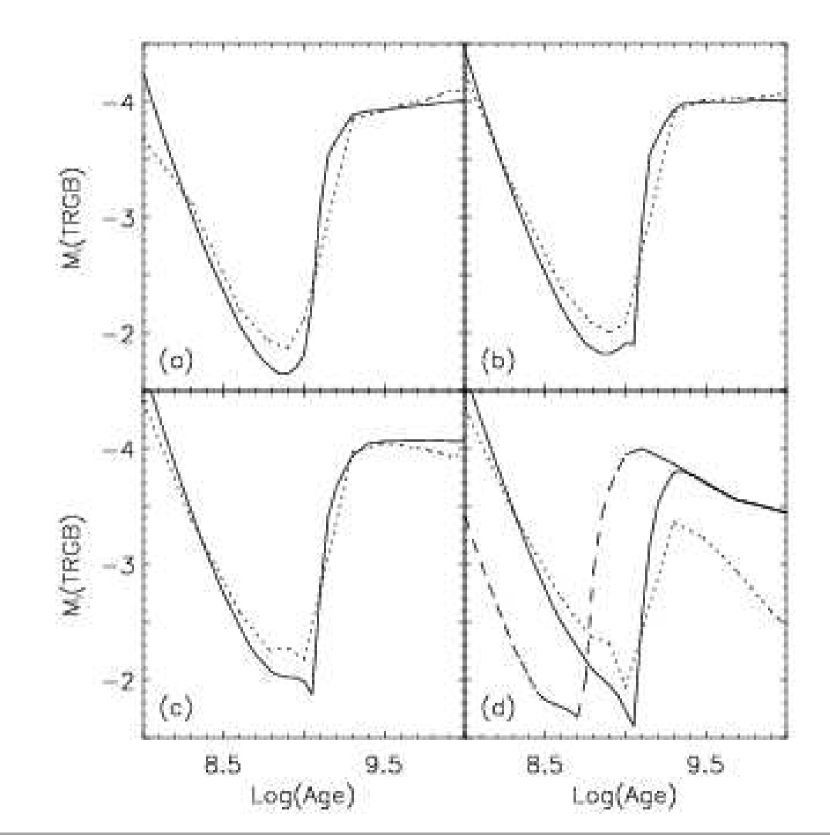
The exact age and duration of the RGB phase transition depends on the details of the stellar models. To demonstrate this point, in Fig. 3 we compare the RGB phase transition of the Padova isochrone set (solid lines) with that of the $\rm Y^{2}$ set (dotted; Yi et al. 2001). The metallicities in panels (a), (b), (c), and (d) are [Fe/H] = -1.7, -1.3, -0.7, and 0.0, respectively. We also show in panel (d) the Padova solar metallicity isochrone with no convective overshoot (dashed). In general, there is good agreement between the $\rm Y^{2}$ and Padova isochrones except for the no overshoot curve in panel (d) which predicts an earlier age and shorter duration for the transition. This is in agreement with Ferraro et al. (1995) who found that models without overshoot predict the transition to occur at $\sim 0.6\pm 0.2$ Gyr and last for $\sim 0.3$ Gyr.

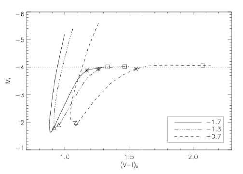
To illustrate how the RGB phase transition could affect the TRGB-distance method, we show in Fig. 4 the evolution of the TRGB in the $\rm M_{I}-(V-I)_{0}$ plane from 0.1 Gyr to 17.8 Gyr. In this figure, ages of 1, 2, and 14 Gyr are marked by triangles, asterisks, and squares, respectively. For ages $\lesssim$ 0.14 Gyr, the TRGB is brighter than $\rm M_{I}=-4.0$ and it evolves to fainter magnitudes until $\sim$ 1 Gyr when the core mass at the TRGB becomes partially degenerate. At these young ages, the TRGB is substantially bluer than the TRGB of ages $>$ 2 Gyr. Hence, it would simply add background noise to a TRGB estimate which could be minimized by excluding stars bluer than a certain color, say $\rm(V-I)_{0}\sim 1.1$ for [Fe/H] = $-1.7$ and $-1.3$ or $\rm(V-I)_{0}\sim 1.3$ for [Fe/H] = $-0.7$. The RGB phase transition occurs approximately between 1 and 2 Gyr. If a stellar population is observed at some point during this stage, the TRGB will be fainter than $\rm M_{I}=-4.0$. One could, in principle, measure the height of the RGB between the red clump (RC) and the TRGB to test if this was the case. However, the RC is not always detected and observational errors could prevent the use of the RGB length as an indicator especially for the late stages of the RGB transition.

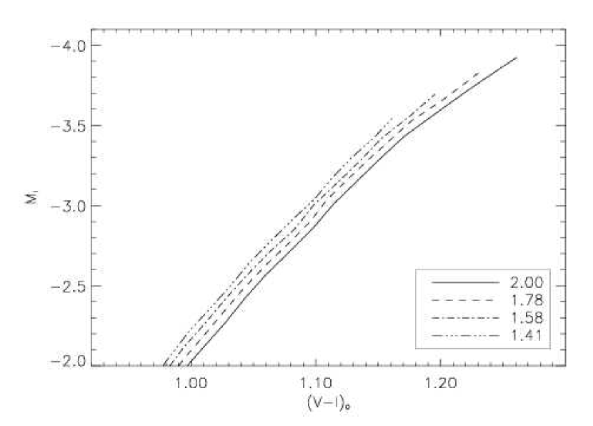
To further illustrate our point, in Fig. 5 we plot the RGBs for [Fe/H] = $-1.3$ and 2, 1.78, 1.58, and 1.41 Gyr. The largest color difference between the RGBs at $\rm M_{I}=-3.0$ is $\sim 0.04$ and the color error at this magnitude is $\sigma_{\rm V-I}\sim 0.07$. Therefore, under typical error conditions, these RGBs would be indistinguishable in the CMD of a galaxy with an unkown distance modulus. We will focus our attention on the ages of 1.58 and 1.78 Gyr when we construct our synthetic CMDs in later sections.

2.4 Determination of $\rm M_{I}(TRGB)$

For each synthetic CMD, we will measure $\rm M_{I}(TRGB)$ and compare it to the calibration from the previous section. At least six different techniques have been used in the literature to measure the magnitude of the TRGB. Each method searches for the discontinuity in the LF of RGB stars corresponding to the TRGB. Lee et al. (1993) introduced the use of the zero-sum Sobel kernel, [$-2$, 0, +2], whose convolution with the LF has a maximum at the largest discontinuity in the LF. Prior to their work, people estimated the TRGB by eye, making it difficult to reproduce and assign errors to their results. A modified Sobel filter was used by Sakai, Madore, & Freedman (1996) with the definition

$$E(m)=\Phi(m+\bar{\sigma})-\Phi(m-\bar{\sigma}),$$ (3)

where $\bar{\sigma}$ is the average photometric error in the range m $\pm$ 0.5 mag and $\Phi$(m) is a Gaussian-smoothed LF calculated as

$$\Phi(m)=\sum^{N}_{i=1}\frac{1}{\sqrt{2\pi}\sigma_{i}}\exp\left[-\frac{(m_{i}-m)^{2}}{2\sigma^{2}_{i}}\right].$$ (4)

In this context, each star has a Gaussian probability distribution centered at the star’s magnitude, $m_{i}$, with dispersion, $\sigma_{i}$. Stars with small errors have more strongly peaked Gaussians than stars with large errors. The total LF is then a sum of all the stars’ Gaussians.

Motivated by the sensitivity of the zero-sum Sobel filter to low-number counts, Frayn & Gilmore (2003) introduced a third method to find the TRGB. They fit a Gaussian cutoff to the LF in the region $\pm$1.0 mag of the Sobel filter’s determination of the TRGB. Their method was found to give more reliable results in the low-number count regime. Yet another method was used by Cioni et al. (2000) who estimated the TRGB to be the maximum of the second derivative of the binned LF plus a small systematic-error correction based on a model for the intrinsic LF. In addition to the Gaussian-smoothed Sobel filter described above, M$\rm\acute{e}$ndez et al. (2002) estimated the TRGB magnitude using the method of maximum likelihood. They maximized the likelihood function on a grid of three parameters, including the magnitude of the TRGB, that described the intrinsic LF of their data. Finally, Sarajedini et al. (2002) used a simple slope-finding algorithm to estimate the TRGB magnitude.

All of the methods described above require a priori knowledge of the general location of the TRGB because there are other features of the LF, such as the red clump, AGB tip, AGB bump (Bellazzini 2002), and RGB bump (Bellazzini 2002; Monaco et al. 2002; Fusi Pecci 1990) which exhibit discontinuities that can be comparable in size to the TRGB. Each method’s accuracy and precision also depend on the signal-to-noise ratio at the TRGB, field-star contamination, and the number of AGB stars near the TRGB. Moreover, all are sensitive to low-number statistics (Madore & Freedman 1995).

Our goal is to test the sensitivity of the TRGB-distance method to variations in SFH rather than compare the different TRGB measurement techniques. Therefore, we simply adopt the technique of Sakai et al. (1997) because it is one of the most commonly used. This method involves applying the Gaussian-smoothed Sobel filter to the logarithmic LF and weighting the filter output by the Poisson noise at each magnitude. This enhances large edges relative to small edges (which are assumed to be noise). The highest peak in the filter response within one magnitude of our theoretically calibrated TRGB is taken to be the true TRGB. To minimize spurious detections due to low-number statistics, we require that at least 1000 stars be present within $\pm 1$ mag of the TRGB in each of our synthetic CMDs. This requirement applies to stars of all ages regardless of SFH so a purely old population will have no stars brighter than the TRGB whereas an intermediate-age population will have many stars brighter than the TRGB. This requirement also means that we must normalize the overall SFRs to high levels not found in the LG dwarf galaxies. However, this is inconsequential to the current study because we are concerned with the relative SFRs at various ages and metallicities. Small numbers of stars near the tip or any of the other problems mentioned above are beyond the scope of this work and have been examined in other papers (Madore & Freedman 1995, Frayn & Gilmore 2003).

To estimate the random error of $\rm M_{I}(TRGB)$, we follow the common technique of using the FWHM of a Gaussian fit to the peak in the edge detector response (Sakai et al. 1999). The total error of each of our TRGB estimates is then given by,

$$\sigma_{tot}^{2}=\sigma_{theory}^{2}+\sigma_{rand}^{2},$$ (5)

where $\sigma_{theory}$ is the standard deviation of $\rm M_{I}(TRGB)$ from the isochrones (0.05; see Fig. 2), and $\sigma_{rand}$ is the random error. For all models, $\sigma_{rand}$ ranges from $0.03-0.09$ and $\sigma_{tot}$ ranges from $0.06-0.11$.

3 The Effect of Age Variations on $\rm M_{I}(TRGB)$

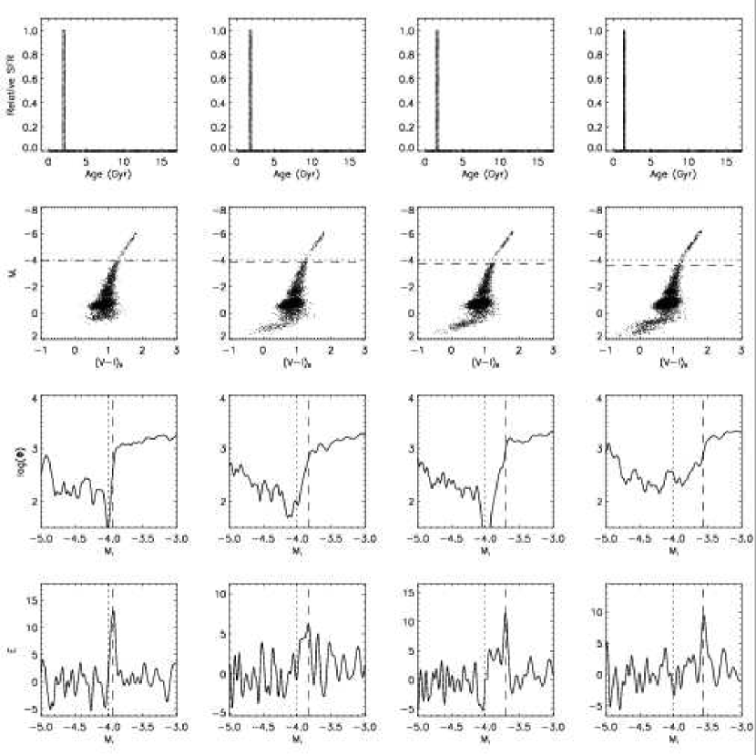
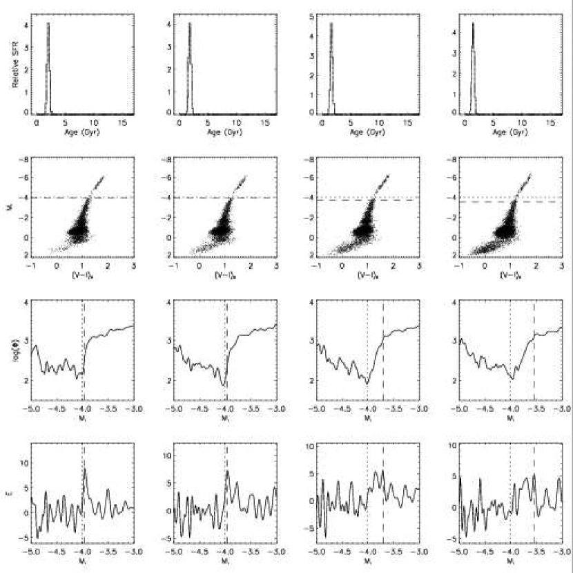
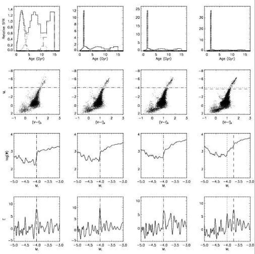
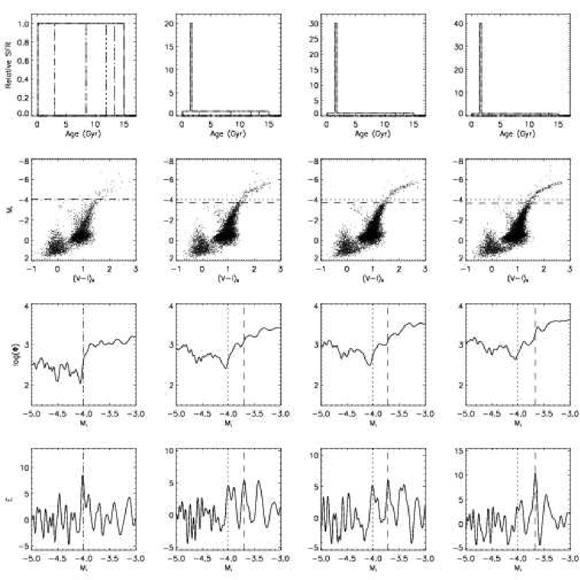
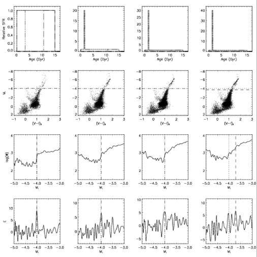
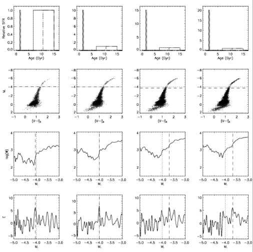
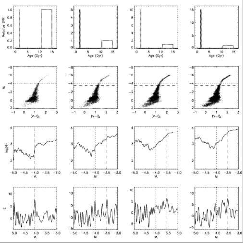
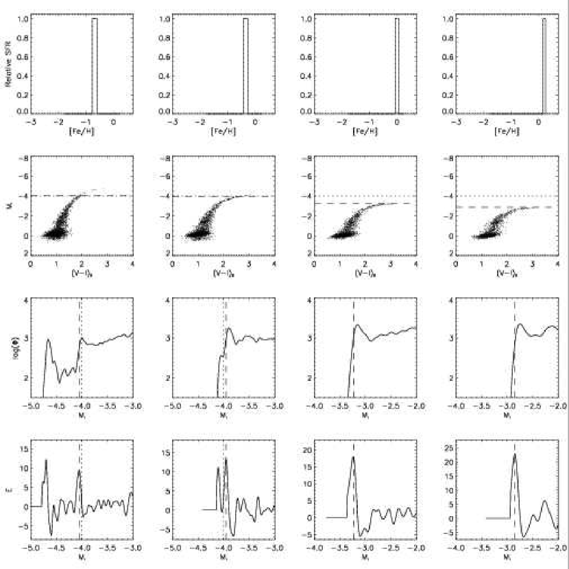
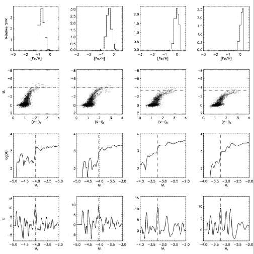
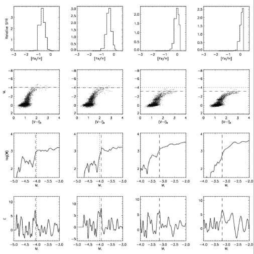
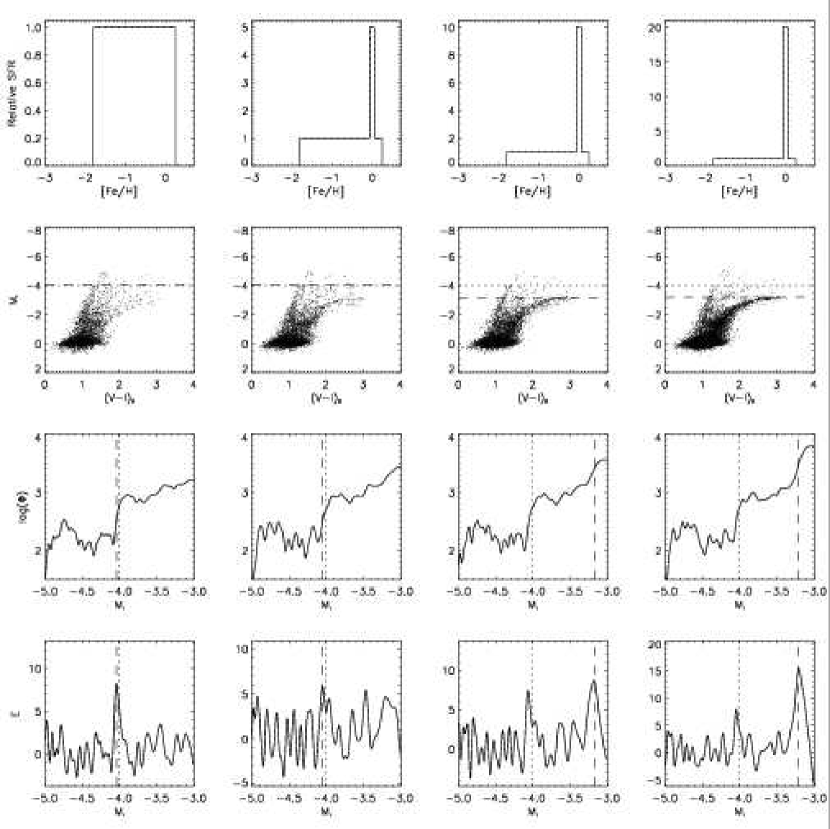
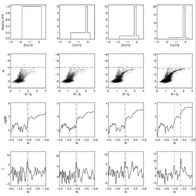
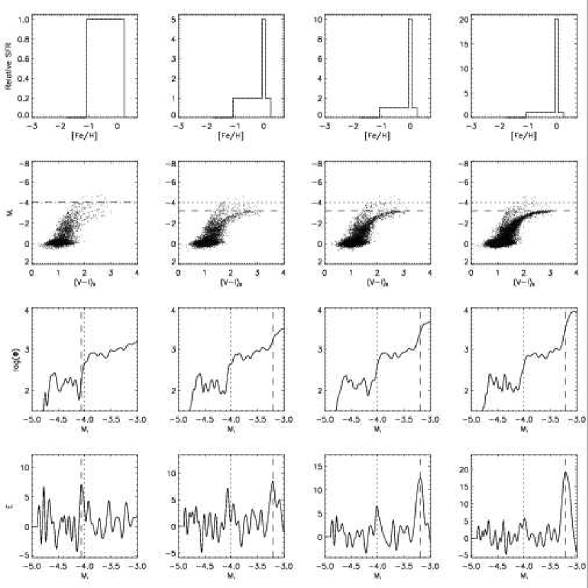
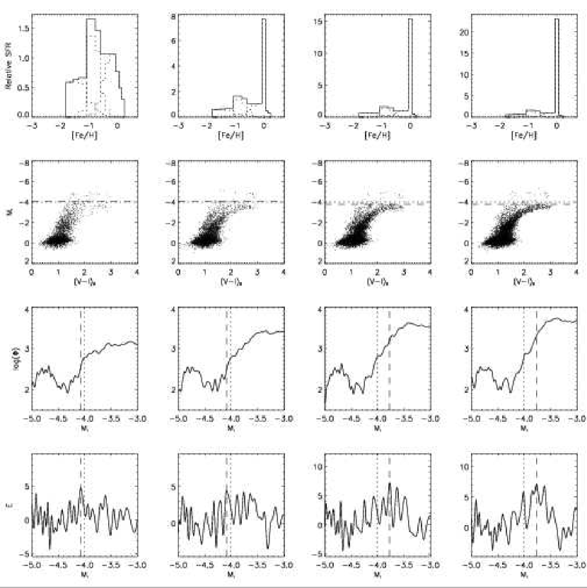
For each of the models discussed below, we plot the relative SFR normalized to the average background rate, the resulting synthetic CMD containing 10% of the stars, logarithmic LF, and edge detector output. The dashed line marks the position of the estimated TRGB value while the dotted line marks our theoretical calibration of $-4.0$.

3.1 Delta-function bursts

We begin by simulating single-age, single-metallicity bursts at 2, 1.78, 1.58, and 1.41 Gyr each with [Fe/H] = $-1.3$ (Fig. 6). Even when observational effects are taken into account, the TRGB becomes fainter as the age decreases. Since there is only one age in each case, the edge detector has no trouble accurately picking out the TRGB as can be seen by comparing the results with the theoretical isochrones of Fig. 5. Each TRGB estimate is well defined and unambiguous.

It is worth noting the gap between the TRGB and the AGB. It is evident as a lack of stars in the CMDs and a depression in the LF just above the TRGB. This gap is important because its presence makes it easier for the edge detector to find the TRGB by reducing the background level of AGB stars. The gap is not an artifact of the method but rather it is intrinsic to the isochrones which predict very rapid evolution on this part of the AGB. Interestingly, such a gap has been observed in Sextans B (Fig. 6 of M$\rm\acute{e}ndez$ et al. 2002) and the Magellanic Clouds (Fig. 5 of Cioni et al. 2000).

3.2 Single Gaussian bursts

It is possible that a mix of ages could hide the effect described in the previous subsection. To investigate this we generated Gaussian bursts in age centered at the same ages as before, each with standard deviation of 0.2 Gyr and [Fe/H] = $-1.3$ (Fig. 7). The edge detector is most sensitive to the largest discontinuity which is due to the dominant population, in this case the center of each Gaussian. In column 2 of Fig. 7, the presence of older stars pulls the derived TRGB up to a brighter magnitude than the equivalent delta-function burst. So we can expect that as the number of intermediate- and old-age stars increases, the number of young stars needed to significantly change the value of $\rm M_{I}(TRGB)$ also increases. The resulting LFs are smoother and because there are several different “competing” TRGBs (one from each age), the discontinuity at each is smaller. Consequently, the peak in the edge detector output corresponding to the TRGB is not as prominent.

3.3 Multiple Gaussian bursts

We now add another level of complexity by simulating three background Gaussian bursts centered at 14.12, 7.08, and 1.58 Gyr. The oldest burst has a standard deviation of 2 Gyr and [Fe/H] = $-1.7$, the intermediate burst has a standard deviation of 2 Gyr and [Fe/H] = $-1.4$, and the young burst has a standard deviation of 1 Gyr and [Fe/H] = $-1.3$. The SFR is zero outside the range $0.09-14.96$ Gyr. First, each burst has an equal height as depicted in Fig. 8 (column 1). Then we add a short, quick burst by scaling the SFR between 1.33 and 1.68 Gyr to $\sim 12$ times (Fig. 8, column 2), $\sim 25$ times (Fig. 8, column 3), and $\sim 35$ times (Fig. 8, column 4) the average background rate. This young burst is timed so that the stars it forms are undergoing the RGB phase transition at the present time.

In the first and second cases, the TRGB is unambiguously detected very close to $\rm M_{I}=-4.0$. In the third case, when the young, quick burst is scaled to $\sim 25$ times the background, the edge detector responds almost equally to the TRGB for the quick burst (at $\rm M_{I}\sim-3.7$) and the TRGB for the older stars. In the fourth case, the edge detector responds primarily to the TRGB of the young population although the TRGB of the old population is still visible at $\rm M_{I}=-4.0$. In a real stellar population this could easily be mistaken for noise due to AGB stars.

3.4 Constant star formation rate

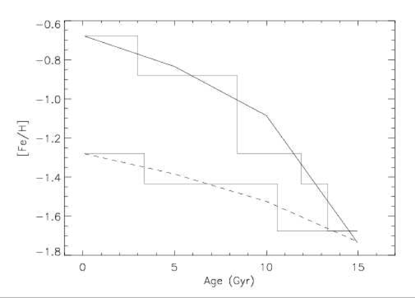
Next we consider a constant SFR from 14.96 to 0.09 Gyr ago. To simulate the metallicity evolution of an LG dwarf galaxy, we use two different chemical enrichment laws (CELs). These laws are plotted in Fig. 9 and described below.

3.4.1 Chemical enrichment law #1

Our first CEL is adapted from Aparicio et al. (1996) for our age range. The metal abundance increases from [Fe/H] = $-1.7$ to $-0.7$. Because our set of isochrones has discrete values of metallicity we approximate the smooth change of [Fe/H] with time by arranging the isochrones into age groups each with constant metallicity.

First, we use a constant SFR (Fig. 10, column 1). Here the TRGB is recovered accurately and precisely. Then we introduce a burst between 1.33 and 1.68 Gyr by scaling the SFR at these ages to 20 times (Fig. 10, column 2) and 30 times (Fig. 10, column 3) the background rate. In both cases, the younger, fainter TRGB is comparable in size to the older, brighter TRGB. Hence, the edge detector responds roughly equally to the TRGBs of the young and old populations but the young TRGB is slightly more dominant. This highlights the importance of careful examination of the edge detector output in the vicinity of the TRGB. If there are peaks of similar size in the output then the random error may be underestimated by simply fitting a Gaussian to the highest peak. Lastly, we scale the young burst up to 40 times the background rate (Fig. 10, column 4). Here the younger, fainter TRGB dominates the edge detector response.

3.4.2 Chemical enrichment law #2

We repeat the procedure from the previous subsection using a different CEL that describes a more gradual metal enrichment (Fig. 9). The only change is that the final metal abundance is decreased to [Fe/H] = $-1.3$. Since the average metallicity of this population is lower than before, the RGB is steeper and the upper AGB is shorter. As before, we start with a constant SFR (Fig. 11, column 1) and add a successively stronger burst between 1.33 and 1.68 Gyr. When the young burst is 20 times (Fig. 11, column 2) and 30 times (Fig. 11, column 3) the background rate, the edge detector appears stable and accurate. When the young burst is 40 times the background rate (Fig. 11, column 4), the edge detector output displays several peaks of comparable height but the highest is due to the TRGB of the young burst.

3.4.3 No intermediate-age stars

If there were no intermediate-age stars, it should be easier for a young burst of star formation to move $\rm M_{I}(TRGB)$ to fainter magnitudes because there would be fewer stars populating the TRGB at $\rm M_{I}=-4.0$. To check this we now investigate what happens when there is a constant SFR from $6.68-14.96$ Gyr and $1.68-1.33$ Gyr with zero SFR everywhere else. The metallicity evolves from [Fe/H] = $-1.7$ for ages $>$ 10.59 Gyr to $-1.4$ for ages between 6.68 Gyr and 10.59 Gyr and then to $-0.9$ for the young burst. We show in Fig. 12 that the TRGB is detected accurately and precisely when the young burst is equal to and 10 times larger than the old SFR. But when the young burst is 15 and 20 times larger, the edge detector responds only to the TRGB of the young burst.

Finally, we repeat the SFH from above except that the SFR between 6.68 Gyr and 10.59 Gyr is set to zero. When the young burst has the same SFR as the old burst the TRGB of the old burst is recovered correctly (Fig. 13, column 1). When the young SFR is scaled to five times the old SFR the discontinuity due to the young TRGB is slightly more significant than that due to the old TRGB (Fig. 13, column 2). The young TRGB dominates the edge detector output when the young SFR is 10 times (Fig. 13, column 3) and 15 times (Fig. 13, column 4) the old SFR.

4 The Effect of Metallicity Variations on $\rm M_{I}(TRGB)$

4.1 Delta-function bursts

As before, we begin with single-metallicity, single-age bursts but we now vary the metallicity and hold the age constant at 10.00 Gyr. This age was chosen to ensure that the effects described in the previous section would not interfere with the results of this section. The burst in Fig. 14 (column 1) has a metallicity of [Fe/H] = $-0.7$. For this case, the largest peak in the edge detector response lies at $\rm M_{I}\sim-4.7$. This peak must be coincident with the AGB tip rather than the TRGB otherwise there would be an unphysically large break in the power-law slope of the RGB LF at $\rm M_{I}\sim-4.0$. Hence, the second-largest peak in the edge detector response which lies at $\rm M_{I}=-4.05\pm 0.06$ must correspond to the TRGB; a fact which we are able to confirm because the masses of the synthetic stars are known.

When the metal abundance is increased to [Fe/H] = $-0.4$ (Fig. 14, column 2), $\rm M_{I}(TRGB)$ is still close to the canonical value but has moved 0.1 mag fainter. Moreover, the slope of the RGB in the CMD has become so shallow that the tip of the AGB occurs at nearly the same magnitude as the TRGB. In the logarithmic LF, the TRGB has almost merged with the tip of the AGB which shows a slightly less significant discontinuity.

In Fig. 14 (column 3), the burst has solar metal abundance. Here there are no AGB stars past the TRGB so the final drop-off in the logarthmic LF is the TRGB rather than the AGB tip. If one were to assume the metallicity of this population was less than $-0.7$, the TRGB brightness would be underestimated by 0.76 mag. An even greater underestimate would occur when [Fe/H] = 0.2 (Fig. 14, column 4), for which the recovered TRGB is over a full magnitude fainter than the canonical value. Note that in these two cases, we had to focus on the magnitude interval $-3.0\pm 1.0$ rather than $-4.0\pm 1.0$ because the slope of the RGB was so shallow.

The four cases above illustrate that the RGB becomes flatter as metallicity increases. This is a well-known phenomenon caused by line blanketing primarily in the V-band but also in the I-band due to the increased metal abundance.

4.2 Single Gaussian metallicity distribution

To investigate the effect of a spread in metallicities we simulated four Gaussian bursts in metallicity each centered on the same metallicities and with the same age as the delta-function bursts. The dispersion of each burst was 0.2 dex. Because our isochrones cover a discrete set of metallicities we can only sample each burst at these metallicities. This results in each CMD having several clearly defined RGBs for each metallicity.

When the Gaussian distribution of metallicities is centered on [Fe/H] = $-0.7$ and $-0.4$, $\rm M_{I}(TRGB)$ lies within 1$\sigma$ of the canonical value (Fig. 15, columns 1 and 2). But when the peak metallicity is [Fe/H] = 0.0 and 0.2 (Fig. 15, columns 3 and 4), the estimated TRGB is about 0.76 mag fainter than the canonical value. In the last case, the TRGB is recovered 0.4 mag brighter than the equivalent delta-function burst. This may be due to the presence of more metal-poor stars populating the TRGB at brighter magnitudes.

Next, we set the SFR in each metallicity bin to be constant from ages $9.44-14.96$ Gyr (Fig. 16). This has the effect of smearing out the RGB of each metallicity. The results are identical except that the recovered TRGB is about 0.1 mag fainter for peak metallicities of [Fe/H] = 0.0 and 0.2.

4.3 Uniform metallicity distribution

Next we examine the case of a uniform metallicity distribution and constant SFR from $9.44-14.96$ Gyr in the past (Fig. 17, column 1). The random error is small and the canonical value lies within the total uncertainty of $\rm M_{I}(TRGB)$. The result is the same when we increase the SFR at solar abundance to five times the background value (Fig. 17, column 2). But at 10 and 20 times the background value (Fig. 17, columns 3 and 4), the edge detector is biased toward the TRGB of this burst. Note that in these latter two cases, the canoncial TRGB due to lower metallicities is still somewhat visible in the edge detector output.

Using the same uniform metallicity distribution and SFR, we repeated the previous procedure but lowered the metallicity of the burst to [Fe/H] = $-0.1$ (Fig. 18). When the burst is five and 10 times stronger than the background rate, the TRGB is close to the canonical value. But when the burst is 20 times the background, $\rm M_{I}(TRGB)$ moves 0.35 mag fainter than the canonical value.

Repeating the procedure with a slightly different metallicity distribution which is uniform but has no stars with [Fe/H] $<-0.9$, the canonical TRGB is recovered to within the total error (Fig. 19, column 1). If the SFR at solar abundance is again increased by a factor of five (Fig. 19, column 2) then the discontinuity due to the TRGB of the burst is larger than that due to the canonical TRGB. When the burst is increased to 10 times (Fig. 19, column 3) and 20 times (Fig. 19, column 4) the background rate the edge detector response is unambiguously biased to fainter magnitudes.

4.4 Multiple Gaussian metallicity distribution

To better simulate the metallicity distribution of real galaxies, we next introduce three Gaussian bursts in metallicity. For the parameters of each Gaussian, we use the metallicity distribution function of Sarajedini & Van Duyne (2001) for M31. The metal-poor component has $\rm[Fe/H]=-1.50\pm 0.45$, the intermediate-metallicity component has $\rm[Fe/H]=-0.82\pm 0.20$, and the metal-rich component has $\rm[Fe/H]=-0.22\pm 0.26$. The SFR at each metallicity is constant and non-zero over the ranges $9.44-14.96$, $5.96-10.59$, and $2.11-6.68$ Gyr for the metal-poor, -intermediate, and -rich components, respectively. Each component is normalized to have equal area but because of our finite metallicity coverage, the metal-rich and metal-poor components are truncated.

In this case (Fig. 20, column 1) the dominant population observed today has $\rm[Fe/H]\sim-0.8$ and age $\sim$ 6 Gyr so $\rm M_{I}(TRGB)$ is $1\sigma$ brighter than the canonical value. But when we introduce a burst at [Fe/H] = 0.0 by scaling the SFR up to $\sim 8$ times larger than the average background rate (Fig. 20, column 2), the edge detector output is ambiguous because it is dominated by several different peaks of nearly equal height. When the same metal-rich burst is scaled to $\sim 15$ times (Fig. 20, column 3) and $\sim 25$ times (Fig. 20, column 4) the average background rate, the edge detector is biased toward fainter magnitudes.

5 Results

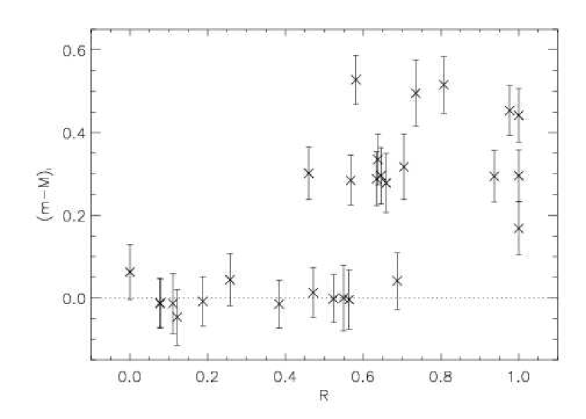
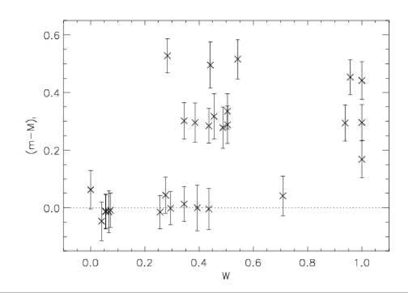
As a quantitative measure of the importance of young stars, we introduce the ratio, $R$, of the number of stars in the RGB phase transition stage within $\pm 1$ mag of the measured TRGB to the total number of stars in the same magnitude range. In Fig. 21 we plot the measured distance modulus assuming $\rm M_{I}(TRGB)=-4.0$ as a function of R. If the young population is small, then $\rm(m-M)_{I}$ is correctly recovered at 0.0. When R $\sim$ 0.50, the young population is half the total population near $\rm M_{I}=-4.0$ and the two competing discontinuities are relatively comparable in size. At this point the edge detector responds to both roughly equally. For R $>$ 0.60, the young population dominates the LF and the TRGB method is inaccurate, leading to overestimates of $\rm(m-M)_{I}$ by $0.2-0.5$ mag.

The quantity, R, is not observable in practice. We would like to use another quantity that provides the same information about the accuracy of the TRGB-distance method but is directly observable. For this purpose, we use the height of the discontinuity at the TRGB, $c$. For each model we make separate linear fits to the logarithmic LF in the regions one magnitude fainter and brighter than the measured TRGB. Then $c$ is simply the difference between the value of each line at the TRGB. This definition of $c$ is similar to that of $\rm M\acute{e}ndez$ et al. (2002), the only difference being ours involves a fit to the observed LF while theirs involves a fit to the intrinsic LF.

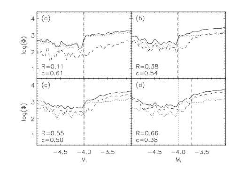
We would expect that as the number of stars undergoing the RGB phase transition increases the TRGB discontinuity of the older population at $\rm M_{I}=-4.0$ eventually disappears in the AGB of the young population. Moreover, the TRGB of the young population is diminished by the RGB of the older population. Hence, for a mix of ages, $c$ should decrease as R increases. In other words, the LF in the vicinity of $\rm M_{I}=-4.0$ should get smoother as R increases. This is demonstrated in Fig. 22 which shows the LFs of the models from §3.3. The same relationship cannot be true for purely young populations because they contain no stars with discordant values of $\rm M_{I}(TRGB)$ to smooth their LFs.

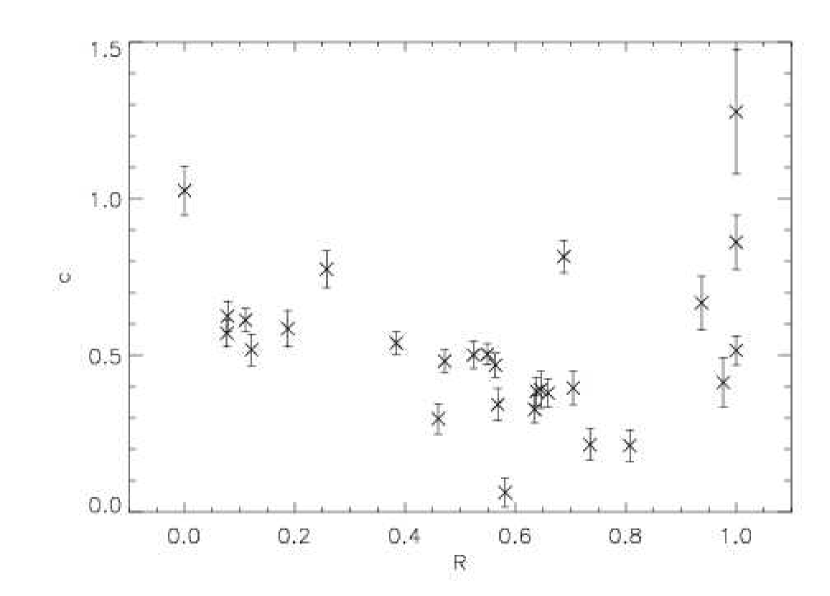
Such is the case in Fig. 23 where we plot $c$ as a function of R. In this plot, the error bars are the random errors of the fit parameters added in quadrature. The purely young models (R $>$ 0.9) do not follow any relationship whereas the models with a mix of ages show an inverse relationship like the one we would expect. To check the strength of the correlation we compute Kendall’s Tau rank correlation coefficient, $\tau$, for all the models and then for just the models with R $<$ 0.9. In the former case, $\tau=-0.18$ indicating a negative correlation exists at the 91% confidence level. In the latter case, $\tau=-0.52$, indicating a negative correlation exists at the 99.96% confidence level. By inspection, values of $c\lesssim$ 0.4 correspond to R $\gtrsim$ 0.55. Hence, values of $c\lesssim$ 0.4 should give errant measurements of $\rm(m-M)_{I}$.

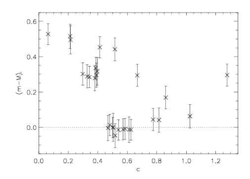
This expectation is confirmed in Fig. 24 which shows our estimated distance modulus as a function of $c$. Models with $c\lesssim$ 0.4 do indeed overestimate $\rm(m-M)_{I}$ by about $0.3-0.5$ mag corresponding to a fractional distance error of $\sim 15-25\%$. Note that we have lost some information in the transition from R to $c$ because values of $c\gtrsim$ 0.4 do not guarantee an accurate estimate of the TRGB. However, $c$ is the more useful parameter because it is directly available from the LF. Finally, large photometric errors at the magnitude of the TRGB could cause a similar smoothing effect to that discussed above.

As another diagnostic, we define the critical SFR, $\rm SFR_{crit}$, as the SFR of a burst between 1 and 2 Gyr ago which causes the TRGB-distance method to fail. This critical SFR is measured relative to the average background rate and depends on the duration of star formation at older ages. When the background star formation occurs over the lifetime of the Universe, $\rm SFR_{crit}\sim 20-40$ (Figs. 8, 10, and 11). If the background star formation ended about 7 Gyr ago, then $\rm SFR_{crit}=15$ (Fig. 12) but $\rm SFR_{crit}=5$ for a background that ended about 10 Gyr ago (Fig. 13). If there were little or no stars created at older ages then $\rm SFR_{crit}\sim 1-4$ (Figs. 6 and 7). When the SFR between 1 and 2 Gyr ago equals $\rm SFR_{crit}$, the distance modulus could be overestimated by $\sim 0.2-0.5$ mag.

In addition to the duration of star formation at old ages, $\rm SFR_{crit}$ also depends on the duration of the burst between 1 and 2 Gyr ago. For example, if the burst was 0.1 Gyr rather than 0.4 Gyr long, $\rm SFR_{crit}$ would be larger. To account for varying strengths and durations of star formation at old and young ages, we define the ratio, $W$, of the number of stars formed $1-2$ Gyr ago to the total number of stars formed over the lifetime of the Universe. In contrast to $R$, $W$ measures the number of stars formed $1-2$ Gyr ago rather than the number of such stars that are observable today in a particular location of the CMD. In Fig. 25, we plot the measured distance modulus versus $W$. When $W>0.30$ there is a 78% chance of overestimating the distance modulus.

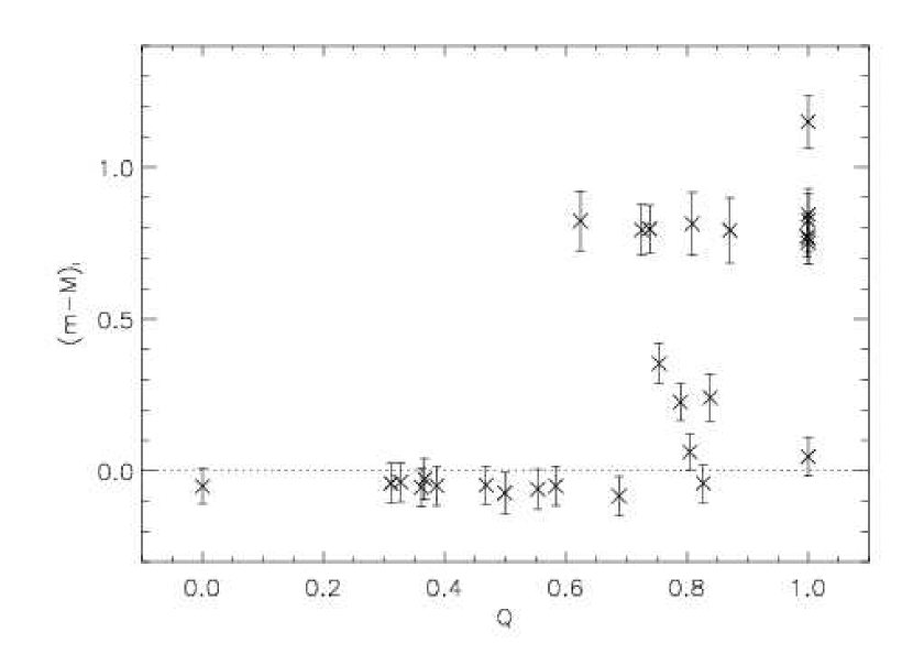
We can understand the effect of metal-rich stars in a similar manner by defining the ratio, $Q$, of the number of metal-rich stars (i.e. [Fe/H] $>-0.7$) located within $\pm 1$ mag of the measured TRGB to the total number of stars in the same magnitude range. In Fig. 26, we plot the distance modulus assuming $\rm M_{I}(TRGB)=-4.0$ as a function of Q. The method is accurate up to Q $\sim$ 0.6 at which point significantly errant measurements begin to occur. In fact, 78% of the measurements with Q $>$ 0.6 are overestimated by $>0.2$ mag.

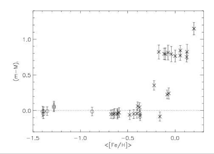
We can also directly explore how the metallicity of stars affects the TRGB distance method. This is shown in Fig. 27 where $\rm\langle[Fe/H]\rangle$ is defined as the average metallicity of stars in the range $0.4-0.6$ mag fainter than the estimated $\rm M_{I}(TRGB)$ for each model. This magnitude range corresponds to $\rm M_{I}=-3.5\pm 0.1$ in the absence of any other information about the true distance modulus. Several models from §3 (column 1 of Figs. $6-8$ and $10-13$) are plotted as open circles to extend the coverage to lower metallicities. The estimated distance modulus is accurate up to $\rm\langle[Fe/H]\rangle\sim-0.3$. Above this metallicity the distance modulus is overestimated by about $0.2-1.0$ mag.

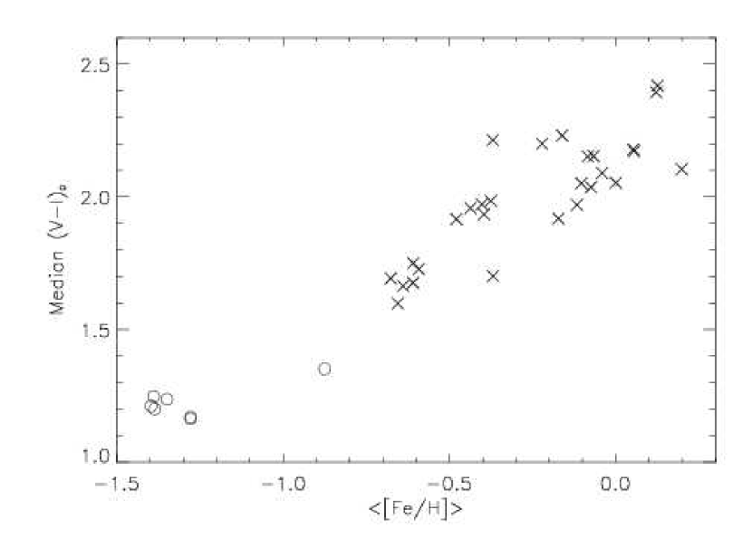
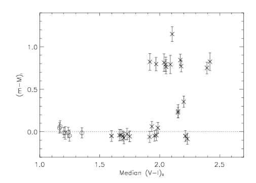
It is more useful to relate the error in distance modulus to a directly observable quantity. Hence, we plot in Fig. 28 the median $\rm(V-I)_{0}$ versus $\rm\langle[Fe/H]\rangle$ for stars $0.4-0.6$ mag fainter than $\rm M_{I}(TRGB)$. Again, the open circles represent several models from §3. As expected, this confirms the well known relation between the color of the TRGB and metallicity. This graph shows that $\rm\langle[Fe/H]\rangle>-0.3$ corresponds to median $\rm(V-I)_{0}\gtrsim$ 2.0. So we would expect that the models with median $\rm(V-I)_{0}\gtrsim$ 2.0 have values of $\rm M_{I}(TRGB)$ significantly different from the canonical value.

This expectation is confirmed in Fig. 29 which shows the distance modulus as a function of the median $\rm(V-I)_{0}$. The distance moduli of all models with median $\rm(V-I)_{0}<1.9$ were recovered accurately but 67% of the models with median $\rm(V-I)_{0}>1.9$ and 86% with median $\rm(V-I)_{0}>2.0$ yielded distance moduli too large by about $0.2-1.0$ mag.

Now we define $\rm SFR_{crit}$ as the SFR of a burst with [Fe/H] $>-0.3$ required to cause the TRGB-distance method to fail. This critical SFR is measured relative to the average background rate at lower metallicities and depends on the range of low metallicities present in the metallicity distribution. When the background star formation occurs for $\rm-1.7\leq[Fe/H]\leq-0.3$, then $\rm SFR_{crit}\sim 10-20$ (Figs. 17, 18, and 20). If the background star formation occurs over a less extended range of metallicities, like $\rm-0.9\leq[Fe/H]\leq-0.3$, then $\rm SFR_{crit}=5$ (Fig. 19). If there were little or no stars created at low metallicities then $\rm SFR_{crit}\sim 1-2$ (Figs. $14-16$). When the SFR at [Fe/H] $>-0.3$ equals $\rm SFR_{crit}$, there is aproximately a 78% chance that the distance modulus will be overestimated by $\sim 0.2-1.0$ mag. This assumes that the SFR at each metallicity is constant over approximately the same amount of time. If the star formation for [Fe/H] $<-0.3$ occurs over a shorter time span, then $\rm SFR_{crit}$ would be reduced.

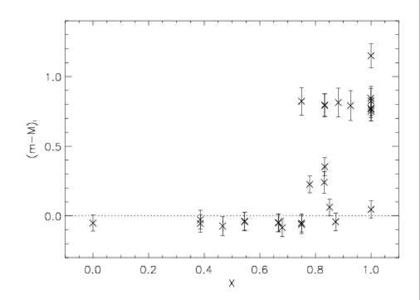
In addition to the range of low metallicities created, $\rm SFR_{crit}$ also depends on the range of high metallicites created. For example, if the burst at high metallicities was 0.1 dex rather than 0.2 dex wide, $\rm SFR_{crit}$ would be larger. To account for varying strengths and widths of metal-poor and -rich bursts, we define the ratio, $X$, of the number of stars created with [Fe/H] $>-0.3$ to the total number of stars created at all metallicities. Unlike $Q$, $X$ measures the number of metal-rich stars formed rather than the number of such stars observable today in a particular location in the CMD. In Fig. 30, we plot the measured distance modulus versus $X$. When $X>0.70$ there is a 71% chance of overestimating the distance modulus.

Tables 1 and 2 summarize the results of all simulations. The last column in both tables is the fractional distance error.

6 Summary and Conclusions

We have shown that the TRGB-distance method is insensitive to star formation history except for large bursts between ages of about 1 and 2 Gyr. Stars formed at these ages are today undergoing the RGB phase transition during which time the TRGB lies at magnitudes fainter than the canonical value. Stars less than 1 Gyr old reach the TRGB at a significantly bluer location in the $\rm M_{I}-(V-I)_{0}$ CMD than stars greater than 2 Gyr old. These very young stars should not significantly affect the TRGB-distance method because they simply add background noise which could be minimized by excluding them from the analysis as is often already done (Jerjen & Rejkuba 2001; Ma$\rm\acute{i}$z-Apell$\rm\acute{a}$niz et al. 2002; Sakai et al. 2000; Sakai et al. 1999; M$\rm\acute{e}$ndez et al. 2002). The RGB length is so short for $1-1.3$ Gyr that one could detect such a population, if the photometry reveals the RC, by measuring the full length of the RGB between the TRGB and RC. But for the middle and late stages of the RGB phase transition ($\sim 1.3-1.7$ Gyr), observational errors might prohibit the use of the RGB length as an indicator.

Instead, the size of the discontinuity, $c$, in the LF at the TRGB can be used as a rough indicator of a large burst between $\sim 1.3-1.7$ Gyr provided that at least 10% of the population was formed well over 2 Gyr ago. If $c\lesssim$ 0.4 then there may be a significant population undergoing the RGB phase transition which comprises at least $\sim$ 60% of the total number of stars within one magnitude of the TRGB. These stars would dominate the LF and the assumption that $\rm M_{I}(TRGB)\approx-4.0$ would cause an overestimate of the distance modulus.

Equivalently, if the strength and duration of star formation between the ages of 1.3 and 1.7 Gyr are such that over 30% of the total number of stars created are created in this age range, then there is a 78% chance the distance modulus will be overestimated by $\sim 0.2-0.5$ mag. This corresponds to a distance error of $\sim 10-25\%$.

When the number of stars with [Fe/H] $>-0.7$ is at least $\sim$ 60% of the total number of stars within one magnitude of the TRGB, there is a $\sim 78\%$ chance they will move $\rm M_{I}(TRGB)$ significantly fainter than the canonical value. This means that when the average metallicity of stars 0.5 mag fainter than the TRGB is $>-0.3$, or alternatively, when the median $\rm(V-I)_{0}$ of these stars is greater than 1.9, $\rm M_{I}(TRGB)$ could be about $0.2-1.0$ mag fainter than $\rm M_{I}=-4.0$. We caution that the RGBs of the isochrones we have used in this study tend to be about 0.2 mag bluer than empirical RGBs. Therefore, in practice the critical color is probably closer to 2.1.

If the strength and duration of star formation at [Fe/H] $>-0.3$ are such that over 70% of the total number of stars created have [Fe/H] $>-0.3$, then there is aproximately a 71% chance the distance modulus will be overestimated by $\sim 0.2-1.0$ mag. This corresponds to a distance error of $\sim 10-45\%$.

Two final notes of caution deserve to be mentioned again. First, the precise age and duration of the RGB phase transition depend on the isochrones used. In particular, models without convective overshoot tend to predict a somewhat earlier age and shorter duration. Second, the sensitivities of the TRGB to variations in SFH which we have examined may change under error, completeness, and crowding conditions significantly different from those we have assumed. This is an issue that deserves further study.

Nevertheless, it is hard to imagine how such strong bursts localized in such a small range of ages or metallicities could actually occur in nature. Indeed, no such bursts have been found in the SFHs of the LG dwarf galaxies (Harris & Zaritsky 2001; Tolstoy et al. 1998; Gallart et al. 1996a; Gallart et al. 1996b; Schulte-Ladbeck et al. 2002; Lynds et al. 1998; Gallart 2000; Carrera et al. 2002; Dolphin 2002). We, therefore, conclude that distance estimates using the TRGB method up to this time have not fallen victim to the effects discussed in this paper. However, as we continue to resolve stellar populations that were previously too far to resolve, it is possible that nature will surprise us yet again.

Figure 1: Photometric error in $\rm M_{V}$ and $\rm M_{I}$ (upper panel) and completeness fraction as a function of $\rm M_{V}$ (lower panel).

Figure 2: I-band absolute magnitude of the TRGB as a function of age from the summary tables of the Padova isochrones. [Fe/H] is given in legend at lower right.

Figure 3: Comparing the RGB phase transition of the Padova isochrones (solid) with that of the $\rm Y^{2}$ isochrones (dotted) for metallicities of (a) [Fe/H] = -1.7, (b) -1.3, (c) -0.7, and (d) 0.0. The dashed curve in panel (d) corresponds to the Padova isochrone with no convective overshoot.

Figure 4: Evolution of the TRGB in the $\rm M_{I}-(V-I)_{0}$ plane. Triangles mark 1 Gyr, asterisks mark 2 Gyr, and squares mark 14 Gyr. [Fe/H] is given in legend at lower right.

Figure 5: RGBs during late stages of the RGB phase transition. Ages in legend are in Gyr and all have [Fe/H] = $-1.3$.

Figure 6: From top to bottom: SFR normalized to average background rate, CMD containing 10% of the stars, logarithmic LF, and edge detector output. The dashed line is the TRGB estimate while the dotted line is the theoretical fiducial value of –4.0. Models shown are single-age bursts with [Fe/H] = $-1.3$ at 2 Gyr (column 1), 1.78 Gyr (column 2), 1.58 Gyr (column 3), and 1.41 Gyr (column 4).

Figure 7: Same panels as Fig. 6. Models shown are single Gaussian bursts with standard deviation of 0.2 Gyr and [Fe/H] = $-1.3$ centered at 2 Gyr (column 1), 1.78 Gyr (column 2), 1.58 Gyr (column 3), and 1.41 Gyr (column 4).

Figure 8: Same panels as Fig. 6. Column 1: Three Gaussian bursts at ages 14.12 Gyr, 7.08 Gyr, and 2.00 Gyr with standard deviations of 2, 2, and 1 Gyr and metallicities of -1.7, -1.4, and -1.3, respectively. The SFR from $1.33-1.68$ Gyr is $\sim 12$ (column 2), $\sim 25$ (column 3), and $\sim 35$ (column 4) times the average background rate.

Figure 9: Chemical enrichment law #1 (solid line) and #2 (dashed line) with their respective discrete approximations.

Figure 10: Same panels as Fig. 6. Column 1: Constant SFR following CEL #1. The dashed vertical lines denote the boundaries of different metal abundance. Starting from the oldest, they are [Fe/H] = $-1.7$, $-1.4$, $-1.3$, $-0.9$, $-0.7$. The young burst from $1.33-1.68$ Gyr is 20 (column 2), 30 (column 3), and 40 (column 4) times stronger than the background SFR.

Figure 11: Same panels as Fig. 6. Column 1: Constant SFR following CEL #2. The dashed vertical lines denote the boundaries of different metal abundance. Starting from the oldest, they are [Fe/H] = $-1.7$, $-1.4$, $-1.3$. The young burst from $1.33-1.68$ Gyr is 20 (column 2), 30 (column 3), and 40 (column 4) times stronger than the background SFR.

Figure 12: Same panels as Fig. 6. Column 1: Constant SFR. The dashed vertical line in top panel denotes the boundary of different metal abundance: [Fe/H] = $-1.7$ for ages $>$ 10.59 Gyr, [Fe/H] = $-1.4$ for ages from $6.68-10.59$ Gyr and [Fe/H] = $-0.9$ for the burst from $1.33-1.68$ Gyr. The young burst from $1.33-1.68$ Gyr is 10 (column 2), 15 (column 3), and 20 (column 4) times stronger than the background SFR.

Figure 13: Same panels as Fig. 6. Column 1: Constant SFR. The metallicities are [Fe/H] = $-1.7$ for ages $>$ 10.59 Gyr and [Fe/H] = $-0.9$ for the burst between 1.33 Gyr and 1.68 Gyr. The young burst from $1.33-1.68$ Gyr is five (column 2), 10 (column 3), and 15 (column 4) times stronger than the background SFR.

Figure 14: Same panels as Fig. 6. Models shown have an age of 10.00 Gyr and [Fe/H] = -0.7 (column 1), -0.4 (column 2), 0.0 (column 3), and 0.2 (column 4).

Figure 15: Same panels as Fig. 6. Models shown have an age of 10.00 Gyr and Gaussian metallicity distribution with dispersion of 0.2 dex centered at [Fe/H] = -0.7 (column 1), -0.4 (column 2), 0.0 (column 3), 0.2 (column 4).

Figure 16: Same panels as Fig. 6. Models shown have an age range of $9.44-14.96$ Gyr and Gaussian metallicity distribution with dispersion of 0.2 dex centered at [Fe/H] = -0.7 (column 1), -0.4 (column 2), 0.0 (column 3), 0.2 (column 4).

Figure 17: Same panels as Fig. 6. Column 1: Uniform metallicity distribution over the range $\rm-1.7\leq[Fe/H]\leq 0.2$ for ages of $9.44-14.96$ Gyr. The SFR at [Fe/H] = 0.0 is increased by factors of five (column 2), 10 (column 3), and 20 (column 4).

Figure 18: Same panels as Fig. 6. Column 1: Uniform metallicity distribution over the range $\rm-1.7\leq[Fe/H]\leq 0.2$ for ages of $9.44-14.96$ Gyr. The SFR at [Fe/H] = -0.1 is increased by factors of five (column 2), 10 (column 3), and 20 (column 4).

Figure 19: Same panels as Fig. 6. Column 1: Uniform metallicity distribution over the range $\rm-0.9\leq[Fe/H]\leq 0.2$ for ages of $9.44-14.96$ Gyr. The SFR at [Fe/H] = 0.0 is increased by factors of five (column 2), 10 (column 3), and 20 (column 4).

Figure 20: Same panels as Fig. 6. Column 1: The metallicity distribution has three Gaussian components displayed as dotted lines while the total is displayed as a solid line. The metallicities of each component are $\rm[Fe/H]=-1.50\pm 0.45$, $\rm-0.82\pm 0.20$, and $\rm-0.22\pm 0.26$ while the SFR at each metallicity is constant over the age ranges $9.44-14.96$, $5.96-10.59$, and $2.11-6.68$ Gyr, respectively. The SFR at [Fe/H] = 0.0 is increased to $\sim 8$ (column 2), $\sim 15$ (column 3), and $\sim 25$ (column 4) times the average rate.

Figure 21: Distance modulus assuming $\rm M_{I}(TRGB)=-4.0$ as a function of R which measures the number of young stars near the TRGB (see text for details). Error bars denote the total error, $\sigma_{tot}$, for each model. The dotted line indicates the distance modulus used for all synthetic CMDs. For R $>$ 0.60, the dominance of young stars causes errant measurements of the distance modulus.

Figure 22: Total LF (solid), LF for stars $\geq$ 2 Gyr (dotted) and $<$ 2 Gyr (dashed) for models discussed in §3.3. Dotted vertical line corresponds to $\rm M_{I}(TRGB)=-4.0$ and dashed vertical line is the estimated $\rm M_{I}(TRGB)$. As R increases from (a) to (d), the LF in the vicinity of $\rm M_{I}(TRGB)$ becomes smoother resulting in smaller values of $c$.

Figure 23: Height of the discontinuity, $c$, in the logarithmic LF at the TRGB as a function of R (see text for details). Models with a mix of stellar ages (R $<$ 0.9) are negatively correlated at 99.96% confidence. Models with R $>$ 0.9 follow no relationship because their LFs near $\rm M_{I}(TRGB)$ are not smoothed by the presence of an older, brighter $\rm M_{I}(TRGB)$.

Figure 24: Distance modulus as a function of $c$. Error bars denote the total error, $\sigma_{tot}$, for each model. The dotted line indicates the distance modulus used for all synthetic CMDs. Models with a mix of stellar ages give errant measurements of the distance modulus when $c\lesssim$ 0.40. Purely young models give errant measurements regardless of $c$.

Figure 25: Distance modulus as a function of $W$ which measures the fraction of stars formed over the lifetime of the Universe that are formed $1-2$ Gyr ago. Error bars denote the total error, $\sigma_{tot}$, for each model. The dotted line indicates the distance modulus used for all synthetic CMDs. For $W$ $>$ 0.30, the number of young stars is large enough to cause errant measurements of the distance modulus.

Figure 26: Distance modulus as a function of Q which measures the number of metal-rich stars near the TRGB (see text for details). Error bars denote the total error, $\sigma_{tot}$, for each model. The dotted line indicates the distance modulus used for all synthetic CMDs. For Q $>$ 0.60, the dominance of metal-rich stars causes errant measurements of the distance modulus.

Figure 27: Distance modulus as a function of $\rm\langle[Fe/H]\rangle$, the average metallicity of stars 0.5 mag below the measured TRGB (see text for details). Error bars denote the total error, $\sigma_{tot}$, for each model. The dotted line indicates the distance modulus used for all synthetic CMDs. Models from column 1 of Figs. $6-8$ and $10-13$ are plotted with open circles to extend the coverage to lower metallicities. For $\rm\langle[Fe/H]\rangle>-0.3$, the dominance of metal-rich stars causes errant measurements of the distance modulus.

Figure 28: Median $\rm(V-I)_{0}$ as a function of $\rm\langle[Fe/H]\rangle$. Models from column 1 of Figs. $6-8$ and $10-13$ are plotted with open circles to extend the coverage to lower metallicities. This confirms the well-known relation between the color of the TRGB and metallicity.

Figure 29: Distance modulus as a function of the median $\rm(V-I)_{0}$ of stars 0.5 mag below the measured TRGB (see text for details). Error bars denote the total error, $\sigma_{tot}$, for each model. The dotted line indicates the distance modulus used for all synthetic CMDs. Models from column 1 of Figs. $6-8$ and $10-13$ are plotted with open circles to extend the coverage to lower metallicities. For $\rm(V-I)_{0}>1.9$, the dominance of metal-rich stars causes errant measurements of the distance modulus.

Figure 30: Distance modulus as a function of $X$ which measures the fraction of stars formed at all metallicities that are formed with [Fe/H] $>-0.3$. Error bars denote the total error, $\sigma_{tot}$, for each model. The dotted line indicates the distance modulus used for all synthetic CMDs. For $X>$ 0.70, the dominance of metal-rich stars causes errant measurements of the distance modulus.

Table 1: Age Models

Fig.#	$\rm M_{I}(TRGB)$	$\sigma_{tot}$	$\sigma_{rand}$	R	$c$	$W$	$\rm(m-M)_{I}$	$\frac{\Delta d}{d}$
(Col.#)
6(1)	-3.94	0.07	0.04	0.00	1.03	0.00	0.06	0.03
6(2)	-3.83	0.06	0.04	1.00	0.86	1.00	0.17	0.08
6(3)	-3.70	0.06	0.04	1.00	1.28	1.00	0.30	0.14
6(4)	-3.56	0.06	0.04	1.00	0.52	1.00	0.44	0.20
7(1)	-3.96	0.06	0.04	0.26	0.77	0.28	0.04	0.02
7(2)	-3.96	0.07	0.05	0.69	0.81	0.71	0.04	0.02
7(3)	-3.71	0.06	0.04	0.94	0.67	0.94	0.29	0.14
7(4)	-3.55	0.06	0.03	0.98	0.41	0.96	0.45	0.21
8(1)	-4.01	0.07	0.05	0.11	0.61	0.07	-0.01	-0.01
8(2)	-4.01	0.06	0.03	0.38	0.54	0.26	-0.01	-0.01
8(3)	-4.00	0.08	0.06	0.55	0.50	0.39	0.00	0.00
8(4)	-3.72	0.07	0.05	0.66	0.38	0.49	0.28	0.13
10(1)	-4.01	0.06	0.03	0.08	0.63	0.06	-0.01	-0.01
10(2)	-3.70	0.06	0.04	0.46	0.30	0.34	0.30	0.14
10(3)	-3.72	0.06	0.03	0.57	0.34	0.94	0.28	0.13
10(4)	-3.66	0.06	0.04	0.64	0.39	0.50	0.34	0.15
11(1)	-4.01	0.06	0.03	0.08	0.57	0.06	-0.01	-0.01
11(2)	-3.99	0.06	0.03	0.47	0.48	0.34	0.01	0.01
11(3)	-4.00	0.07	0.05	0.56	0.47	0.44	0.00	-0.00
11(4)	-3.71	0.06	0.04	0.63	0.33	0.50	0.29	0.13
12(1)	-4.05	0.07	0.05	0.12	0.52	0.04	-0.05	-0.02
12(2)	-4.00	0.06	0.03	0.52	0.50	0.29	0.00	0.00
12(3)	-3.70	0.07	0.05	0.65	0.39	0.39	0.30	0.14
12(4)	-3.68	0.08	0.06	0.70	0.40	0.46	0.32	0.15
13(1)	-4.01	0.06	0.03	0.19	0.59	0.07	-0.01	0.00
13(2)	-3.47	0.06	0.03	0.58	0.06	0.28	0.53	0.24
13(3)	-3.50	0.08	0.06	0.73	0.21	0.44	0.50	0.23
13(4)	-3.48	0.07	0.05	0.81	0.21	0.54	0.52	0.24

Table 2: Metallicity Models

Fig.#	$\rm M_{I}(TRGB)$	$\sigma_{tot}$	$\sigma_{rand}$	Q	$\rm\langle[Fe/H]\rangle$	Median	$X$	$\rm(m-M)_{I}$	$\frac{\Delta d}{d}$
(Col.#)						$\rm(V-I)_{0}$
14(1)	-4.05	0.06	0.03	0.00	-0.68	1.69	0.00	-0.05	-0.02
14(2)	-3.95	0.06	0.04	1.00	-0.38	1.98	1.00	0.05	0.02
14(3)	-3.24	0.08	0.06	1.00	0.00	2.05	1.00	0.76	0.35
14(4)	-2.85	0.09	0.07	1.00	0.20	2.10	1.00	1.15	0.53
15(1)	-4.03	0.07	0.05	0.37	-0.59	1.73	0.39	-0.03	-0.01
15(2)	-4.04	0.06	0.04	0.83	-0.40	1.97	0.87	-0.04	-0.02
15(3)	-3.23	0.07	0.05	1.00	0.05	2.18	1.00	0.77	0.36
15(4)	-3.25	0.07	0.05	1.00	0.12	2.39	1.00	0.75	0.35
16(1)	-4.05	0.06	0.04	0.36	-0.61	1.75	0.39	-0.05	-0.02
16(2)	-3.94	0.06	0.03	0.80	-0.40	1.93	0.85	0.06	0.03
16(3)	-3.16	0.07	0.05	1.00	0.05	2.17	1.00	0.84	0.39
16(4)	-3.18	0.10	0.09	1.00	0.13	2.42	1.00	0.82	0.38
17(1)	-4.04	0.06	0.04	0.33	-0.61	1.68	0.54	-0.04	-0.02
17(2)	-4.05	0.06	0.04	0.39	-0.66	1.60	0.67	-0.05	-0.02
17(3)	-3.18	0.10	0.08	0.62	-0.17	1.92	0.75	0.82	0.38
17(4)	-3.21	0.08	0.07	0.73	-0.10	2.05	0.83	0.79	0.37
18(1)	-4.04	0.07	0.04	0.31	-0.64	1.66	0.54	-0.04	-0.02
18(2)	-4.05	0.06	0.04	0.47	-0.44	1.96	0.67	-0.05	-0.02
18(3)	-4.05	0.06	0.04	0.58	-0.37	2.21	0.75	-0.05	-0.02
18(4)	-3.65	0.06	0.04	0.75	-0.22	2.20	0.83	0.35	0.16
19(1)	-4.06	0.07	0.04	0.55	-0.48	1.92	0.75	-0.06	-0.03
19(2)	-3.20	0.08	0.06	0.74	-0.12	1.97	0.83	0.80	0.37
19(3)	-3.19	0.10	0.09	0.81	-0.07	2.04	0.88	0.81	0.37
19(4)	-3.21	0.11	0.09	0.87	-0.04	2.09	0.92	0.79	0.36
20(1)	-4.07	0.07	0.05	0.50	-0.37	1.70	0.47	-0.07	-0.03
20(2)	-4.08	0.07	0.04	0.69	-0.16	2.23	0.68	-0.08	-0.04
20(3)	-3.77	0.06	0.03	0.79	-0.08	2.15	0.78	0.23	0.10
20(4)	-3.76	0.08	0.06	0.84	-0.07	2.15	0.83	0.24	0.11
6(1)	-3.94	0.07	0.04	0.00	-1.28	1.17	0.00	0.06	0.03
7(1)	-3.96	0.06	0.04	0.00	-1.28	1.16	0.00	0.04	0.02
8(1)	-4.01	0.07	0.05	0.00	-1.40	1.21	0.00	-0.01	-0.01
10(1)	-4.01	0.06	0.03	0.00	-0.88	1.35	0.00	-0.01	-0.01
11(1)	-4.01	0.06	0.03	0.00	-1.39	1.20	0.00	-0.01	-0.01
12(1)	-4.05	0.07	0.05	0.00	-1.39	1.25	0.00	-0.05	-0.02
13(1)	-4.01	0.06	0.03	0.00	-1.35	1.24	0.00	-0.01	0.00

Note. — The last seven models are included from Table 1 to extend the coverage to lower metallicities.

References

- (1) Aparicio, A., & Gallart, C. 1995, AJ, 110, 2105
- (2) Bellazzini, M. 2002, Mem. S.A.It., 0, 1.
- (3) Bellazzini, M., Ferraro, F. R., & Pancino, E. 2001, ApJ, 556, 635
- (4) Carrera, R., Aparicio, A., Martnez-Delgado, D., & Alonso-Garca, J. 2002, AJ, 123, 3199.
- (5) Cioni, M.-R. L., van der Marel, R. P., Loup, C., & Habing, H. J. 2000, A&A, 359, 601
- (6) Da Costa, G. S., & Armandroff, T. E. 1990, AJ, 100, 162
- (7) Dolphin, A. E. 2002, MNRAS, 332, 91
- (8) Ferraro, F. R., Fusi Pecci, F., Testa, V., Greggio, L., Corsi, C. E., Buonanno, R., Terndrup, D. M. & Zinnecker, H. 1995, MNRAS, 272, 391
- (9) Frayn, C. M., & Gilmore, G. F. 2003, MNRAS, 339, 887
- (10) Fusi Pecci, F., Ferraro, F. R., Crocker, D. A., Rood, R. T., & Buonanno, R. 1990, A&A, 238, 95
- (11) Gallart, C. 2000, ASP Conf. Ser, vol. 3, D. Alloin, G. Galaz, & K. Olsen, eds.
- (12) Gallart, C., Aparicio, A., Bertelli, G., & Chiosi, C. 1996b, AJ, 112, 2596
- (13) Gallart, C., Aparicio, A., Bertelli, G., & Chiosi, C. 1996a, AJ, 112, 1950
- (14) Girardi, L., Bressan, A., Bertelli, G., & Chiosi, C. 2000, A&AS, 141, 371
- (15) Harris, J., & Zaritsky, D. 2001, ApJS, 136, 25
- (16) Jerjen, H., & Rejkuba, M. 2001, A&A, 371, 487
- (17) Karachentsev, I. D., et al. 2002, A&A, 389, 812
- (18) Lee, M. G., Freedman, W. L., & Madore, B. F. 1993, ApJ, 417, 553
- (19) Lynds, R., Tolstoy, E., O’Neil, Jr., E. J., & Hunter, D. A. 1998, AJ, 116, 146
- (20) Madore, B. F., & Freedman, W. L. 1995, AJ, 109, 1645
- (21) Maz-Apellniz, J., Cieza, L., & MacKenty, J. W. 2002, AJ, 123, 1307
- (22) Mndez, B., Davis, M., Moustakas, J., Newman, J., Madore, B. F., & Freedman, W. L. 2002, AJ, 124, 213
- (23) Monaco, L., Ferraro, F. R., Bellazzini, M., & Pancino, E. 2002, ApJ, 578, 47
- (24) Sakai, S., Madore, B. F., & Freedman, W. L. 1999, ApJ, 511, 671
- (25) Sakai, S., Madore, B. F., & Freedman, W. L. 1996, ApJ, 461, 713
- (26) Sakai, S., Madore, B. F., Freedman, W. L., Lauer, T. R., Ajhar, E. A., & Baum, W. A. 1997, ApJ, 478, 49
- (27) Sakai, S., Zaritsky, D., & Kennicutt, Jr., R. C. 2000, AJ, 119, 1197
- (28) Sarajedini, A., et al. 2002, ApJ, 567, 915
- (29) Sarajedini, A., Van Duyne, J. 2001, AJ, 122, 2444
- (30) Schulte-Ladbeck, R. E., Hopp, U., Drozdovsky, I. O., Greggio, L., & Crone, M. M. 2002, AJ, 124, 896
- (31) Sweigart, A. V., Greggio, L., & Renzini, A. 1990, ApJ, 364, 527
- (32) Tolstoy, E., et al. 1998, AJ, 116, 1244
- (33) Yi, S., Demarque, P., Kim, Y.-C., Lee, Y.-K., Ree, C., Lejeune, T., & Barnes, S. 2001, ApJS, 136, 417