Search for non-Gaussianity in pixel, harmonic and wavelet space: compared and combined
Abstract
We present a comparison between three approaches to test non-Gaussianity of cosmic microwave background data. The Minkowski functionals, the empirical process method and the skewness of wavelet coefficients are applied to maps generated from non-standard inflationary models and to Gaussian maps with point sources included. We discuss the different power of the pixel, harmonic and wavelet space methods on these simulated almost full-sky data (with Planck like noise). We also suggest a new procedure consisting of a combination of statistics in pixel, harmonic and wavelet space.
pacs:
02.50.Ng, 95.75.Pq, 02.50.Tt, 98.80.EsI Introduction
The fluctuations of the cosmic microwave background (CMB) are expected to be close to Gaussian distributed. In view of the increasing quantity of CMB experiments, it is now possible to check this assumption on data with growing resolution and sky coverage. Most models for the early universe predict some small deviations from Gaussianity; non-standard models of inflation Martin et al. (2000); Contaldi et al. (2000); Linde and Mukhanov (1997); Bartolo et al. (2002); Gupta et al. (2002); Gangui et al. (2002); Liguori et al. (2003), cosmic strings (See Ref.Gangui et al. (2001) for a review) and point sources. Detecting these small deviations would be of great importance for the understanding of the physics of the early universe. Also systematic effects like a non-symmetric beam and noise could give rise to non-Gaussian features. For this reason a non-Gaussianity check could reveal whether the impact of the instrumental effects on the data of the experiment is well understood.
The methods to search for non-Gaussianity in the literature mainly concentrate on implementing the test in three different spaces: (1) In pixel space: the Minkowski functionals Novikov et al. (2000); Gott et al. (1990) (which were used to set limits on the non-Gaussianity in the WMAP data Komatsu et al. (2003)), temperature correlation functions Eriksen et al. (2002), the peak to peak correlation function Heavens and Gupta (2000), skewness and kurtosis of the temperature field Scaramella and Vittorio (1991) and curvature properties Doré et al. (2003); Barreiro et al. (2001), to mention a few. (2) In harmonic space: analysis of the bispectrum and its normalized version Phillips and Kogut (2000); Komatsu et al. (2002); Troia et al. (2003); Komatsu and Spergel (2001) and the bispectrum in the flat sky approximation Winitzki and Wu . The explicit form of the trispectrum for CMB data was derived in Hu (2001); Kunz et al. (2001). Phase mapping Chiang et al. . Applications to COBE, Maxima and Boomerang data have also drawn enormous attention and raised wide debate Wu et al. (2001); Polenta et al. (2002); Ferreira et al. (1998); Banday et al. (2000). The empirical process method Hansen et al. (2002, 2003); Marinucci and Piccioni (2004). Finally, (3) wavelet space: Barreiro and Hobson (2001); Barreiro et al. (2000); Gonzalez et al. (2002); Mukherjee et al. (2000). Traditionally, these tests are performed separately in each space. In this article, we will take methods in pixel- (the Minkowski functionals), harmonic- (the empirical process) and wavelet-space (skewness), and we will make a comparison for two different models of non-Gaussianity. We will also combine the methods in order to improve the total power. It should be noted that all the procedures we consider are non-parametric, that is they do not assume any a priori knowledge about the nature of non-Gaussianity.
We will use these methods on 100 maps generated from a non-standard inflationary model Bartolo et al. (2002) and on 100 maps where we have included point sources. We assess the performance of the methods in the different spaces for the different types of non-Gaussianity. We also propose a combined test which turns out to be more robust.
In section II, we review the method of Minkowski functionals, in section III we describe our implementation of the method and in section IV we define our proposed statistic. In section V, we review the empirical process method while section VI is devoted to the wavelets. In section VII the methods are compared and applied to non-standard inflationary models, in section VIII to maps with point sources. Finally in section IX we summarize and comment on our results.
II Minkowski functionals
To analyze a spherical map in terms of Minkowski functionals, we consider the excursion sets, that is, the map subsets which exceed a given threshold value. The threshold is labelled and it is treated as an independent variable, on which these functionals depend. More precisely, considering the normalized random field of temperature fluctuations, we can define the ’hot region’ Q as the ensemble of pixels higher than the level :
| (1) |
The three functionals of interest then are, up to constant factors Minkowski (1903):
1) Area: is the total area of all hot regions.
2) Boundary length: is proportional to the total length of the boundary between cold and hot regions
3) Euler characteristic or genus: , a purely topological quantity, counts the number of isolated hot regions minus the number of isolated cold regions, i.e. the number of connected components in Q minus the number of ’holes’.
The rationale behind these statistics can be explained from mathematical results in Hadwiger (1959); in particular, these results can be interpreted by stating that all the morphological information of a convex body is contained in the Minkowski functionals (Winitzki and Kosowsky, 1997)); here, by morphological we mean the properties which are invariant under translations and rotations and which are additive Tomita (1990); Worsley (1994); Schmalzing and Górski (1998). The three statistics, normalized by the area density, can then be expressed as
| (2) | |||||
| (3) | |||||
| (4) |
where is the contour of the region ; and are the differential elements of and , respectively; is the geodetic curvature of .
The expected values for a given thresholds depends on a single parameter given for a Gaussian field by Tomita (1990):
| (5) | |||||
| (6) | |||||
| (7) |
with :
| (8) |
where semicolon indicates the covariant derivative on the sphere.
In the case of CMB (8) reduces to Schmalzing and Górski (1998):
| (9) |
where is the angular power spectrum.
An immediate consequence of the above formulae is that, although the expected value of the first Minkowski functional is invariant with respect to the dependence structure of , for the second and third Minkowski functional this is not the case and calibration for a given angular power spectrum is needed. Moreover, even for the first Minkowski functional, knowledge of the angular power spectrum is required for a Monte Carlo evaluation of its variance. This can be viewed as a drawback, and because of this some effort has been undertaken to provide at least some crude upper bound for the functionals’ variance (Winitzki and Kosowsky (1997)).
III The Implementation of Minkowski Functionals
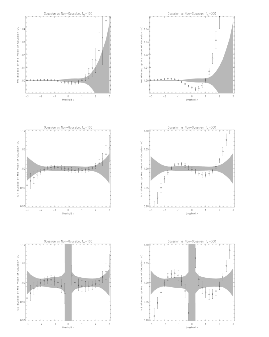
In order to estimate the three functionals we simulate a map of the CMB Górski et al. (1998) with a known power spectrum, and then we cut the maximum number of independent tangent planes of dimension ; in this way it is easy to calculate the values of the three Minkowski functionals in the flat-sky limit, taking into account the possibility of gaps (galactic cut, polar calottes). Due to projection effects, finite pixel size and the dimension of the tangent planes, we find a deviation of the simulated values with respect to the analytical spherical predictions (eqs.5). Note however that the shape of the curves is unaffected, which is not the case when non-Gaussianities are present (see fig. 2). In fig. 1 we show a comparison between analytical expectation values and the values computed on the tangent planes.


IV Test of non-Gaussianity in pixel space
In order to test non-Gaussianity we use a test defined by:
| (10) |
Our procedure is as follows;
-
•
Given an observed map, we estimate the power spectrum.
-
•
Using the estimated power spectrum, we generate 200 Gaussian realizations Górski et al. (1998)
-
•
For each map we calculate the Minkowski functionals, using the tangent planes as described above
-
•
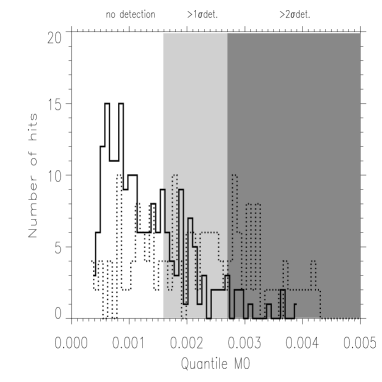
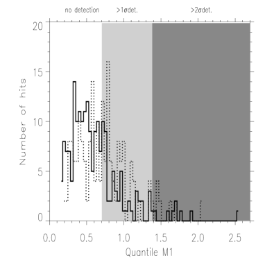
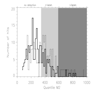
We calibrate the quantiles (i.e. the threshold values at a given significance level) using the Monte Carlo simulations; the one and two sigma detection levels are shown in fig.3.
-
•
We calculate our statistic (10) from the observed map and compare the result with the Monte-Carlo calibration; we are thus able to determine at which confidence level the map is Gaussian or not.


V The empirical process method
The details of the empirical process approach to detect non-Gaussianity in the CMB were given in Hansen et al. (2002, 2003); Marinucci and Piccioni (2004). In short, the method consists of a family of tests which focus on the total distribution of and check for dependencies between -rows. The first step is to transform the spherical harmonic coefficients into variables which have an approximate uniform distribution between and , given that the were initially Gaussian distributed. This is done using the Smirnov transformation, defined as
where is the cumulative distribution function of a with
degrees of freedom and are the power spectrum coefficients
estimated from the data. The error introduced by using estimated instead of the real underlying is dealt with using a
bias-subtraction, as described in Hansen et al. (2002).
Then the joint empirical distribution function for row is formed,
where determines the spacing between the rows for which the dependencies are tested and denotes the difference in for row . The parameters run over the interval . The empirical process is expressed using the centered and rescaled given as
The intuition behind this procedure is as follows: if the s are Gaussian, converges to a well-defined limiting process, whose distribution can be readily tabulated. On the other hand, for non-Gaussian s and thereby will take ‘high’ values over some parts of -space. Thus, the analysis of some appropriate functional of can be used to detect non-Gaussianity. To combine the information over all multipoles into one statistic, we define
| (11) |
where is the highest multipole where the data is signal dominated.
The method can then be summarized as follows: the distribution of is found using Monte-Carlo simulations of Gaussian distributed . Then, for a given observed set of , the value is found and compared to the distribution obtained from Monte-Carlo. The consistency of the data with a Gaussian distribution can then be estimated to any suitable -level. In Hansen et al. (2003) this simple approach was extended in three different ways. First of all, the fact that the above explained estimator is not rotationally invariant is exploited, using the value averaged over many rotations. Each rotation can be viewed as a resampling of the . Secondly, we introduced three variations of the test, taking into account, not only the modulus of the but also the phases. Finally, experimental effects like noise and galactic cut was accounted for using Monte Carlo calibration of the distribution with these effects included. It should be noted that the rotated maps are clearly dependent and the resulting statistic may thus depend on the shape of the angular power spectrum.
VI Test of non-Gaussianity in wavelet space
A third space where one could look for non-Gaussianity is the wavelet space. The use of wavelets for non-Gaussianity tests of the CMB has been investigated by several authors Barreiro and Hobson (2001); Barreiro et al. (2000); Gonzalez et al. (2002); Mukherjee et al. (2000) and turns out to be a very powerful tool. We will here just briefly describe the wavelet method, and refer to the above references for more details.
An isotropic wavelet can be defined as
| (12) |
with the properties
| (13) |
| (14) |
where , R represents a scale and b a translation. The Fourier transform of the wavelet is represented by . We will focus on the mexican hat wavelets given by:
| (15) |
From the wavelet transform of a function one can obtain the wavelet coefficients :
| (16) |
and if is Gaussian, will be Gaussian as well. We will here use the CMB temperature fluctuation field as the function. We will implement the non-Gaussianity test in wavelet space as we did for the Minkowski functionals:
-
•
we generate a set of Gaussian CMB maps for calibration and a set of non-Gaussian maps for testing
-
•
we cut tangent planes
-
•
we calculate for each plane the coefficients
-
•
we evaluate the skewness of the wavelet coefficients for each sky.
-
•
finally, using the skewness of the wavelets from the Gaussian maps, we define the one and two detection levels as described above for the other methods.
VII Comparison and combined test
This section aims at comparing the different methods described above.
Applying the methods on the same maps , we will first compare the number of detections. We will in this paper use the non-standard inflationary model described in Bartolo et al. (2002); Liguori et al. (2003) which has the non-linear coupling parameter as a measure of the strength of non-Gaussianity. We generated 100 ‘observed’ skies with Planck-like noise (LFI 100 GHz), beam 20’, pixel-size 6’ (Nside 512 in Healpix language), using a pure Sachs-Wolfe spectrum with values of 300 and 100. In figures 2, 4 and 5 one can see the behavior of the Minkowski functionals in the presence of a non-zero . In tables 1 and 2 we show the rejection rates. As the first Minkowski
functional was giving the best results in this tests, we will
focus only on for this kind of non-Gaussianity. In table 3 we list the results of the wavelet test on the same maps (for the wavelets we used the parameter ). For individual results of the empirical process test, we refer to Hansen et al. (2003).
| quantile detection limits | ||||||||
|---|---|---|---|---|---|---|---|---|
| 3.6 | 0.286 | 33.2 | ||||||
| 6.3 | 0.524 | 49.7 | ||||||
| Rejection rates | ||||||||
| 100% | 100% | 100% | ||||||
| 100% | 71% | 84% | ||||||
| quantile detection limits | ||||||||
|---|---|---|---|---|---|---|---|---|
| 3.6 | 0.286 | 33.2 | ||||||
| 6.3 | 0.524 | 49.7 | ||||||
| Rejection rates | ||||||||
| 68% | 52% | 57% | ||||||
| 35% | 8% | 8% | ||||||
| 100 | |
|---|---|
| Confidence Level | Rejection Rate |
| 1 | 89% |
| 2 | 57% |
Table 4 shows the number of detections at the different
levels, using and the empirical process method on maps with and . The power of the two procedures appears very close. However, analyzing the individual maps, we find
that only one third of the maps detected at are the same for the
two tests. This leads to the idea of implementing a combined test.
| TEST | emp. proc | comb | |||
|---|---|---|---|---|---|
| 100 | 300 | 100 | 300 | 100 | |
| 1 | 50% | 95% | 68% | 100% | 74% |
| 2 | 29% | 87% | 35% | 100% | 35% |
For the combined test we suggest to use an indicator consisting of from the Minkowski functionals and from the empirical process. We chose to normalize the and so that they both have mean zero and variance one, using Monte-Carlo simulations of Gaussian maps. In this way, the two values can be averaged:
| (17) |
where
| (18) |
and
| (19) |
Here means mean value taken over 100 Gaussian simulations.
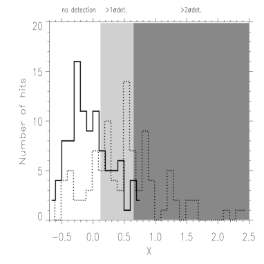
The weights and were chosen proportionally to the power of each procedure. Using the rejection rates for in table 2, we arrived at and . Of course, the threshold value for needs to be evaluated anew. In figure (6) we plot the distribution of for the Gaussian and non-Gaussian maps.
By a similar motivation, it is natural to combine also the wavelet method into a single procedure; it is easy to see (tables 2 and 3) that the detection rate at is about two times higher for the wavelets, warranting the wavelet coefficient a very high weight in the combined analysis. Inspecting table 4, we detect a moderate improvement in the detection rate when combining Minkowski functionals and empirical process. The result of the empirical process + Minkowski functionals + wavelets combined test is shown in table 5. A significant improvement of the number of detections at both confidence levels is evident; note that the combined procedure is to some extent model dependent, as the weights we used were tabulated from specific non-Gaussian models.
| 100 | |
|---|---|
| Confidence Level | Rejection Rate |
| 1 | 100% |
| 2 | 78% |
VIII Point sources
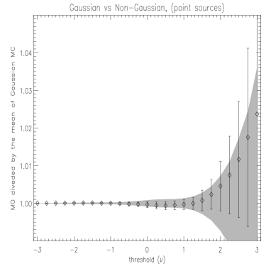
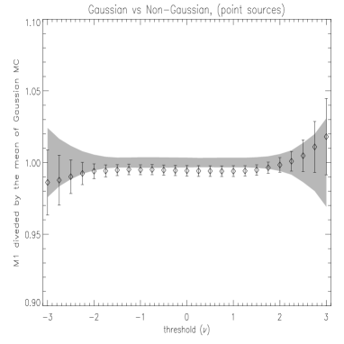
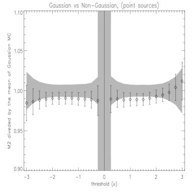
We also simulated maps with point sources (with noise and beam as given above) to compare the power of the methods on a different kind of non-Gaussianity. We generated a toy model of point sources with a distribution building on formula (1) in Pierpaoli (2003) and formulae (1) and (2) in Tegmark and de Oliveira-Costa (1998). In table 6 we show the results for the Minkowski functionals. We see immediately that for this kind of non-Gaussianity, the first Minkowski functional is not sensitive, whereas the other two functionals show a good rejection rate. This suggests that we might be able to discriminate between these two types of non-Gaussianity. The first Minkowski functional can be used to trace primordial non-Gaussianity with little influence from the point sources. On the other hand, the presence of point sources will show up in the second and third Minkowski functionals, which are only weakly influenced by primordial non-Gaussianity. In Figure (7) we show the shape of the Minkowski functionals in the presence of point sources. Note that the deviations from the Gaussian mean are different than in the case of primordial non-Gaussianity (Figure 4). The point sources manifest themselves mainly as an offset in and , consistent with what was observed for weak lensing Schmalzing et al. (2000). However as seen in figure (5) for non-standard inflation the curve has a particular shape.
One could imagine combining and in order to strengthen the power of the test, similarly to what we have done above. However, it turns out that the maps detected by are contained within the maps detected by , so that there is no additional information in combining the two estimators.
| quantile detection limits | ||||||||
|---|---|---|---|---|---|---|---|---|
| 1.1 | 0.415 | 207.6 | ||||||
| 1.7 | 0.770 | 328.3 | ||||||
| Rejection rates | ||||||||
| 36% | 81% | 75% | ||||||
| 8% | 45% | 33% | ||||||
For the empirical process method, there was no detection for any of the tests, univariate, bivariate or trivariate. The numbers obtained for the maps with point sources were consistent with those for Gaussian maps. Also for the wavelet test, the number of detections was very small. Note that wavelets can be useful for detection of bright point sources Cayón et al. (2000), but in our source model these were excluded. This might suggest that the empirical process methods and the skewness of the wavelets can be used to probe primordial non-Gaussianity without confusion from point sources, making the combined test presented above more robust.
IX Comments and conclusions
We have compared three methods for detecting non-Gaussianity in observations of the cosmic microwave background. The methods were applied to non-Gaussian maps with two different kinds of non-Gaussianity, primordial non-Gaussianity with a varying and point sources. It is important to note that the non-Gaussian maps used in this article were generated taking into account only the Sachs-Wolfe effect. In future work we will study maps where the full radiative transfer equations have been applied. For the time being, we stress that our results are broadly consistent with the power of the procedures adopted for WMAP data analysis. More precisely, a detailed comparison is unfeasible, as we are assuming a simplified non-Gaussian model (no radiative transfer) and Planck LFI like noise and beam. Moreover we are restricting the analysis to the first 500 multipoles . Broadly speaking, however, Monte-Carlo simulations suggest that a value of about 100 represents the lower limit that can be detected at a level, by using a combined procedure: this seems consistent with the value reported in (Komatsu et al. (2003)). As an estimator of non-Gaussianity for the Minkowski functionals we have introduced a statistic which gathers the information from different thresholds (eq.10). The estimator for the empirical process method is , the maximum value of the function obtained from a given map (eq.11) using the trivariate test. For the test in wavelet space, we use the skewness of wavelet coefficients.
For the primordial non-Gaussianity, and the empirical process method have a similar rejection rate, whereas and showed less power. On the other hand, for the maps with point sources, and gave the best results, whereas and the empirical process method had no rejections. The fact that the first Minkowski functional shows little power in the presence of point sources is hardly surprising. Indeed this statistic depends only on the pixel by pixel temperature values and hence is not at all affected by discontinuities in the map. The converse is clearly true for the other Minkowski functionals, which are sensitive to the local morphology of the maps. For the empirical process, we simply note that spikes in real space are erased in harmonic space. It is also important to stress that our results depend heavily upon the nature of non-Gaussianity; in particular some preliminary exploration of Monte-Carlo evidence from non-physical toy models suggests that the power of these procedures need not be close, in general. This strengthens the case for (weighted) multiple/combined procedures; the combined procedures seem to show a marked improvement in the power of the test. However, the pixel-, harmonic- and wavelet-space methods, despite carrying complementary statistical information, should not be viewed neither as orthogonal nor as independent, so that some care is needed when merging them into a single statistic. In any case, the fact that different methods detect different kinds of non-Gaussianity can be viewed as an advantage, in the sense that, for instance, primordial non-Gaussianity can be detected without confusion from point sources.
Acknowledgements.
We are thankful to Michele Liguori and Sabino Matarrese for supplying maps with primordial non-Gaussianity. We also wish to thank Paolo Natoli for suggestions and useful discussions. This research used resources of the National Energy Research Scientific Computing Center, which is supported by the Office of Science of the U.S. Department of Energy under Contract No. DE-AC03-76SF00098. We acknowledge the use of the Healpix package Górski et al. (1998).References
- Martin et al. (2000) J. Martin, A. Riazuelo, and M. Sakellariadou, Phys. Rev. D61, 083518 (2000).
- Contaldi et al. (2000) C. R. Contaldi, R. Bean, and J. Magueijo, Phys. Lett. B468, 189 (2000).
- Linde and Mukhanov (1997) A. Linde and V. Mukhanov, Phys. Rev. D56, 535 (1997).
- Gupta et al. (2002) S. Gupta, A. Berera, A. F. Heavens, and S. Matarrese, Phys. Rev. D66, 043510 (2002).
- Gangui et al. (2002) A. Gangui, J. Martin, and M. Sakellariadou, Phys. Rev. D66, 083502 (2002).
- Bartolo et al. (2002) N. Bartolo, S. Matarrese, and A. Riotto, Phys. Rev. D65, 103505 (2002).
- Liguori et al. (2003) M. Liguori, S. Matarrese, and L. Moscardini, ApJ 597, 57 (2003).
- Gangui et al. (2001) A. Gangui, L. Pogosian, and S. Winitzki, Phys. Rev. D64, 043001 (2001).
- Novikov et al. (2000) D. Novikov, J. Schmalzing, and V. F. Mukhanov, A&A 364, 17 (2000).
- Gott et al. (1990) J. R. Gott et al., ApJ 352, 1 (1990).
- Komatsu et al. (2003) E. Komatsu et al., ApJS 148, 119 (2003).
- Eriksen et al. (2002) H. K. Eriksen, A. J. Banday, and K. M. Górski, A&A 395, 409 (2002).
- Heavens and Gupta (2000) A. F. Heavens and S. Gupta, MNRAS 324, 960 (2000).
- Scaramella and Vittorio (1991) R. Scaramella and N. Vittorio, ApJ 375, 439 (1991).
- Doré et al. (2003) O. Doré, S. Colombi and F. R. Bouchet MNRAS 344, 905 (2003).
- Barreiro et al. (2001) R. B. Barreiro, E. Martinez-Gonzalez, and J. L. Sanz, MNRAS 322, 411 (2001).
- Phillips and Kogut (2000) N. G. Phillips and A. Kogut, ApJ 548, 540 (2000).
- Komatsu et al. (2002) E. Komatsu, B. D. Wandelt, D. N. Spergel, A. J. Banday, and K. M. Górski, ApJ 566, 19 (2002).
- Komatsu and Spergel (2001) E. Komatsu and D. N. Spergel, Phys Rev. D63, 063002 (2001).
- Troia et al. (2003) G. D. Troia et al., MNRAS 313, 284 (2003).
- (21) S. Winitzki and J. H. P. Wu, eprint astro-ph/0007213.
- Hu (2001) W. Hu, Phys. Rev. D64, 083005 (2001).
- Kunz et al. (2001) M. Kunz et al., ApJ 563, L99 (2001).
- (24) L. Y. Chiang, P. Naselsky, and P. Coles, eprint astro-ph/0208235.
- Wu et al. (2001) J. H. Wu et al., Phys. Rev. Lett. 87, 251303 (2001).
- Polenta et al. (2002) G. Polenta et al., ApJ Lett. 572, L27 (2002).
- Ferreira et al. (1998) P. G. Ferreira, J. Magueijo, and K. M. Górski, ApJ 503, L1 (1998).
- Banday et al. (2000) A. J. Banday, S. Zaroubi, and K. M. Górski, ApJ 533, 575 (2000).
- Hansen et al. (2002) F. K. Hansen, D. Marinucci, P. Natoli, and N. Vittorio, Phys. Rev. D66, 063006 (2002).
- Hansen et al. (2003) F. K. Hansen, D. Marinucci, and N. Vittorio, Phys. Rev. D67, 123004 (2003).
- Marinucci and Piccioni (2004) D. Marinucci and M. Piccioni, Ann. Stat. 32, 3 (2004).
- Barreiro and Hobson (2001) R. B. Barreiro and M. P. Hobson, MNRAS 327, 813 (2001).
- Barreiro et al. (2000) R. B. Barreiro, M. P. Hobson, A. N. Lasenby, A. J. Banday, K. M. Gorski, and G. Hinshaw, MNRAS 318, 475 (2000).
- Gonzalez et al. (2002) E. M. Gonzalez, J. E. Gallegos, F. Argueso, L. Cayon, and J. L. Sanz, MNRAS 336, 22 (2002).
- Mukherjee et al. (2000) P. Mukherjee, M. P. Hobson, and A. N. Lasenby, MNRAS 318, 1157 (2000).
- Minkowski (1903) H. Minkowski, Math. Ann. 57, 447 (1903).
- Worsley (1994) K. J. Worsley, Adv. Appl. Prob. 26, 13 (1994).
- Schmalzing and Górski (1998) J. Schmalzing and K. M. Górski, MNRAS 297, 355 (1998).
- Tomita (1990) H. Tomita, Formation, Dynamics and Statistics of patterns, ed. K. Kawasaki, M. Suzuki, A. Onuki, Vol 1 (World Scientific), 113-157 (1990).
- Górski et al. (1998) K. M. Górski, E. Hivon, and B. D. Wandelt, Analysis Issues for Large CMB Data Sets’, 1998, eds A. J. Banday, R. K. Sheth and L. Da Costa, ESO, Printpartners Ipskamp, NL, pp.37-42 (1998).
- Pierpaoli (2003) E. Pierpaoli, ApJ 589, 58 (2003).
- Tegmark and de Oliveira-Costa (1998) M. Tegmark and A. de Oliveira-Costa, ApJ 500, L83 (1998).
- Schmalzing et al. (2000) J. Schmalzing, M. Takada, and T. Futamase, ApJ 544, L83 (2000).
- Cayón et al. (2000) L. Cayón et al., MNRAS 315, 757 (2000).