Wide-field millimagnitude photometry with HAT:
A Tool for Extra-solar Planet Detection

Abstract

We discuss the system requirements for obtaining millimagnitude photometric precision over a wide field using small aperture short focal length telescope systems, such as are being developed by a number of research groups to search for transiting extra-solar planets. We describe the Hungarian-made Automated Telescope (HAT) system which attempts to meet these requirements. The attainable precision of HAT has been significantly improved by a technique in which the telescope is made to execute small pointing steps during each exposure so as to broaden the effective point spread function of the system to a value more compatible with the pixel size of our CCD detector. Experiments during a preliminary survey (Spring 2003) of two star fields with the HAT-5 instrument allowed us to optimize the HAT photometric precision using this method of PSF broadening; in this way have been able to achieve a precision as good as 2 millimagnitudes on brighter stars. We briefly describe development of a network of HAT telescopes (HATnet) spaced in longitude.

1 Introduction

The discovery of the transiting planet HD 209458b (Charbonneau et al., 2000; Henry et al., 2000) was a landmark in exoplanet research. It established that at least some substellar companions to stars found in close orbits ($\sim$ 0.05 AU) by radial velocity techniques really are gas giants planets, with mass and radius comparable to theoretical expectations for a “hot Jupiter”, that is, with radius of order 35% larger than expected for a Jupiter-mass gas giant planet orbiting at several AU from the star. Because HD 209458 is a relatively close and bright star (I band magnitude 7.0), detailed follow-up observations were possible, and those from HST  (Brown et al., 2001) yielded the first measurements of its atmospheric sodium composition, showing it to be broadly consonant with theoretical expectations (Charbonneau et al., 2002); the existence of a hydrogen exosphere (Vidal-Madjar et al., 2003); as well as detailed stellar-planet system parameters (Queloz et al., 2000). Thus the star’s brightness has allowed us to explore the physics of an extrasolar planet atmosphere years ahead of expectations. In recognition of this, we have embarked on a survey for additional examples of planets transiting nearby bright stars, using a small Hungarian-made Automated Telescope (HAT) system.

Many projects searching for transiting giant planets have sprung up since the discovery of HD 209458b, and can be divided in two main types: deep and narrow surveys use medium to large size telescopes with a narrow field-of-view (FOV) to record many faint sources, while wide and shallow surveys use small telescopes with a wide FOV to record a great number of bright nearby stars (see Horne, 2003, for a comprehensive list of such projects). The charm of small telescopes is that instrumentation is affordable, even allowing building dedicated instruments for the project and thus, assuming robust automation, having practically unlimited telescope time. Furthermore, if a transiting candidate is found, the brightness of the parent star enables prompt follow-up observations (both photometric and spectroscopic) with 1m-class telescopes to determine whether the candidate is worth further investigation with large and unique facilities (10m class telescopes and HST ), or whether it is a false positive mimicking a transit for other reasons. However, the results so far have been disappointing, since (as of this writing) no detections have yet been announced using these wide-field surveys. While this has given rise to some skepticism about whether they will ever bear fruit, this skepticism is unwarranted; it is simply the case that earlier projections of the detection rate (e.g. Horne, 2003) were overly optimistic – perhaps by as much as a factor of 10 (Brown, 2003). In fact, the only planet discovered by the transit method (OGLE-TR-56b), and not by radial velocity searches, belongs to the “deep and narrow” surveys, as it was found with the 1.3m OGLE telescope at $I\approx 16$ (Udalski et al., 2002; Konacki et al., 2003; Torres et al., 2003).

A useful discussion of expected detection and false alarm rates for transiting Jovian planets has been given in Brown (2003). These rates can be calculated by combining two terms. The first is an empirical estimate on the probability that a star with magnitude $m_{0}$ (and color index $C_{0}$) harbors a transiting Jovian planet with period P, fractional transit duration q and photometric depth $\delta$. This distribution function also depends on some secondary parameters such as galactic latitude $b$ and longitude $l$, which relate to the distribution of stellar types (hence radii), as well as field crowding and thus false alarm rates. The second term comes from the capabilities of the survey: photometric precision $\sigma$ as a function of $m_{0}$, number of data-points accumulated for a star and their distribution in time, and angular resolution of the imaging. For completeness, there is also a third term, which is the data reduction method used for filtering the transit candidate light-curves from the flood of data.

The combination of these terms yields a joint probability distribution, which tells what the chance is that a single star ($m_{0}$, $C_{0}$, $l$, $b$) has a bona-fide transit (with characteristics P, q, $\delta$) and gets selected when the specific transit-search algorithm is run on the accumulated data (with given number of data points and time distribution) collected by the survey that is characterized by its photometric capabilities. Naturally, the above joint probability has to be integrated over the number of stars observed by the survey. In this paper we concentrate on the “observational” term of the probability distribution, i.e. on how to optimize the characteristics of our ongoing HAT survey in order to maximize the number of expected detections, with special focus on the optimizing photometric precision through a PSF-broadening (PB) technique.

Throughout this paper, by (photometric) “precision” we will refer to the repeatability of the measurements for the same star, i.e. the rms of the JD versus magnitude time-series (light-curve). The light-curves are established by relative photometry, essentially using differential magnitudes based on most of the bright stars in the field. Because of the nature of the search for photometric variations that are not known a priori, a great number of such stars are used as comparison stars through an iterative and robust procedure of rejecting outliers, and finding the frame to frame magnitude offsets. For clarity, we distinguish between the repeatability as described above, and the accuracy of the relative magnitude measurements within a single frame. The latter is characterized by the difference between measured magnitude values for the same virtual star if placed at different XY positions on a single frame. Finally, accuracy of the standard photometry describes the relation of the instrumental magnitude system, which is characteristic to the project, to the standard photometric system, such as that of Landolt (1992).

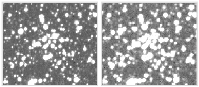
Figure 3: A $25\arcmin\times 25\arcmin$ region (approx 1/300th of a frame) showing the open cluster M34 taken by HAT-6 with tracking mode (left, 1.2 pix FWHM) and PSF broadening mode (right, 2.0 pix FWHM). Blurring is to the eye only slight, but makes a significant difference in photometry.

Given the expected depth of only $\sim 1\%$ of hot Jupiter transits, photometric precision of time-series measurements plays a critical role in detection capabilities (Brown, 2003, Fig. 3). However, achieving adequate ($\leq 1\%$) precision of the light-curves over a wide FOV projected on a front-illuminated CCD, and on data coming from an unattended automated instrument, poses serious technical challenges, which might be partly the reason for the negative results so far of wide-field surveys. These challenges are discussed in §2.

In order to make HAT suitable for extra-solar giant planet transit detection, and improve our precision, several hardware modifications were performed on the prototype HAT-1 system (Bakos et al., 2002). Section §3 gives an overview on these, and §4, describes our PB-technique that has improved our precision still further. The upgraded, new-generation HAT, called HAT-5, was started up early 2003 at the Smithsonian Astrophsical Observatory’s Fred L. Whipple Observatory (FLWO), Arizona, and has been running since. Sections §5 and §6 summarize our observations taken in the Spring season of 2003 with HAT-5, and data reduction steps relevant to achieving the photometric precision. We compare our photometry taken with standard “tracking” mode and the PB-technique in §7, and explain why PB yields better performance. The resulting short and long-term photometric precision, as well as systematic variation in the light-curves are discussed in the same section. In §8 we describe our experience with the BLS transit search method based upon the 91-night dataset of the above Spring season, and also show sample light-curves. Finally, in §9, we summarize the precision obtained with HAT-5, and touch upon future prospects of the HATNet - a multi-element network consisting of identical instruments, which has been operational since November, 2003. Further information can be found at the HAT homepage.

2 Photometric precision with a wide-field, short focus instrument

As stated earlier, photometric precision of time-series measurements is a key factor in detection capabilities. Although the events searched for are periodic, the loss in precision (characterized by $\sigma$, the rms observed magnitude variation of a constant star) is difficult to overcome by increasing the number of data points, $N_{obs}$: the detection chance is roughly proportional to $\sqrt{N_{obs}}/\sigma$. Furthermore, the number of data points per star that can be accumulated (in a year) is obviously limited by the seasonal visibility of fields. Improving the precision per data point rather than increasing $N_{obs}$ facilitates detecting a potential transit early in an observing season, so as to allow follow-up observations that same season. Naturally, photometry at the level of 1% or better can contribute strongly to general stellar variability studies in addition to exoplanet transit searches, for it enables study of otherwise undetectably low-amplitude variables.

Achieving precision better than 1% over an extended FOV poses serious technical challenges. The following complications that arise in astrometry and photometry for a typical, low-budget planet search project are marked with two-character symbols for future reference (see Table 1 for a summary).

Wide Field Issues (W): The requirement of a wide FOV in order to observe a large number of bright sources translates into short focal length for moderate sized CCD detectors. This plus the need for reasonable aperture to maximize the incoming flux, results in rather fast focal ratio instruments (for example f/1.8 lenses in the HAT project). As a result, the geometry of the focal plane is significantly distorted, so that astrometry is more complicated than with “conventional” telescopes (W1). In addition the stellar profiles are far from perfect, and change significantly over the wide FOV (W2). This gets worse with even slight defocusing, and the fast focal ratio increases the difficulty of achieving satisfactory focus. (W3). Even matching frames of the same instrument can be problematic due to differential refraction (W4), e.g. a corner of the field is “lifted-up” at high zenith angles. Finally, differential extinction (W5) across the field can be considerable at high zenith angles.

Flat-fielding Issues (F): Commercially available telephoto lenses exhibit strong vignetting (both optical and geometrical), typically having only 60-80% incoming intensity in the corners compared to that of the center of the field. While this is in principle corrected by flatfielding, residual large-scale flatfielding errors are proportional to the amount of the correction and hence can be significant (F1). The many lens elements (the HAT lenses consist of 12 lens elements in 10 groups) cause reflected stray-light patterns (F2) to appear on the images, and further decrease flatfielding precision. The sky background is variable (F3) over a typically few degree scale, both spatially and in time (Chromey & Hasselbacher, 1996), so that skyflats do not truly represent the transmission function of the system on large-scale, and median combining is problematic, so that small-scale errors are more enhanced than at large telescopes (F4). Due to the short focus, and depth-of-field (close objects are not completely out of focus), it is virtually impossible to find any setup for domeflat exposures.

Sky Noise and Undersampling Issues (S & U): With typical CCD pixel sizes of $\sim 14\mu$ and focal lengths of $\sim 200\,mm$, the pixels correspond to large area on the sky (e.g. $14\arcsec\times 14\arcsec$), and hence sky-background is one of the major contributors to noise (S1). For wide field short focal length lenses such as we employ, the optical point spread function (PSF) has a full width at half maximum (FWHM) of order 20″. Hence the stellar profiles are undersampled on the CCD chip. This involves several further complications, the most prominent being the increased effect of residual small-scale flatfield errors in the photometry (U1). Most methods for finding the centers of sources start to break down below $\sim$2 pix FWHM (U2). Undersampled profiles cause problems for both PSF-fitting (U3), and flux-conserving image interpolation (U4) to a reference frame. Finally, the maximum star brightness before pixel saturation occurs at fixed exposure time is less if the PSF is narrow and undersampled (U5). This limits photometric precision due to additive (per frame) noise-terms, such as readout-noise.

Merging Issues (M): Merging of stellar sources is increased not only by the fast focal ratio and limited resolving power of the optics, but also by the undersampled profiles (M1). While at first approximation, a constant, time-independent merging of sources on the frames would not harm the photometric precision of a time-series measurement, any intrinsic variation exhibited by one of the stars (e.g. a shallow transit) is suppressed by the flux contribution of nearby sources. However, even a constant merging affects the precision through centroid and sky-background determination errors. Furthermore, even with perfect telescope pointing, if the PSF and hence merging of sources is variable in time, then the the relative brightness of stars varies from frame to frame (M2).

Other CCD Issues (C): If only semi-professional (but affordable), front illuminated CCDs are used, this poses further difficulties. For example, the HAT project uses Apogee AP10 2K$\times$2K, front illuminated camera with 14$\mu$ pixels. The gate and channel structure in front of the pixels causes an unknown intra-pixel (C1) and inter-pixel (C2) variability (Buffington, Booth, & Hudson, 1991). The dark-current with such, typically Peltier-cooled systems is not negligible (C3).

Depending on the goals of the photometry, and the stability of the instrument, such as pointing precision and focusing stability, different subsets of the above effects are important. In the following we distinguish between “major” (few tens of pixels), “minor” (a few pixels) and sub-pixel (better than few tenths of a pixel) pointing accuracy, and nightly or long-term photometric precision. Some of the effects, such as S1, M1 and U2-5, are simply present in general, irrespectively of the above categories.

If one performs absolute astrometry of the fields, i.e. cross identifies stars with a catalogue, then W1, W4, U2, U3 and M1-2 have to be dealt with. Relative astrometry between frames from the same instrument will generally depend on the same effects, except for dependence on distortion of the optics (W1), if the pointing errors are “minor” or better.

Relative photometry is the typical application needed by transit-search projects to generate time-series of stars. In an ideal setup, if the fields were observed with sub-pixel pointing precision and constant PSF width at the same night (and reduced with the same flatfield), the photometric precision (but not the accuracy) would be almost indifferent to all the problematic effects except those generally present for photometry (W5, S1, M1, U2-5). However, because W4 (differential refraction) causes displacement of the centroids, even at perfect tracking and polar alignment, sub-pixel positioning is possible only in a limited part of the field, and over a limited hour angle range. Thus relative photometry with even excellent pointing (e.g. through auto-guiding) is still slightly affected by F4, U1, C1-2, and with increasing pointing errors their contribution is amplified. If pointing accuracy is even worse than “minor” (i.e. a few tens of pixels), then virtually all the remaining effects have to be dealt with. If focusing stability is poor, which is usually relevant to long-term precision, then variable merging (M2) is also a significant contributor to noise in crowded fields.

Finally, absolute photometry and calibration of fields to a standard system suffers from almost all the above problems. For example large-scale flatfielding errors (F1), field-position dependent profiles (W2), and stray-light (F2) can cause up to $\sim 5\%$ absolute calibration errors.

Issue	Short explanation
Wide Field
W1	Distorted geometry in astrometry
W2	Spatially variable stellar profiles
W3	Sensitivity of profiles to focusing
W4	Differential refraction
W5	Differential extinction
Flat-fielding
F1	Strong vignetting, uncertainty of large corrections
F2	Stray-light patterns
F3	Variable sky background
F4	Increased small-scale flatfield errors
Sky Noise and Undersampling
S1	High sky background per pixel
U1	Increased effect of residual flatfield errors
U2	Imprecise centroid fitting
U3	Breakdown of psf fitting
U4	Problematic image interpolation
U5	Limited flux for brightest unsaturated stars
Merging
M1	Increased merging
M2	Time-dependent merging due to change in profiles

Table 1: Issues in wide-field astrometry and photometry

3 History and current hardware

The development of HAT was initiated by Bohdan Paczyński in 1999 with the original purpose being all-sky variability monitoring. HAT is a small automated observatory, incorporating a robotic horseshoe mount, a clamshell dome, a large-format CCD, a telephoto lens, and auxiliary devices, all controlled by a single PC running RealTime Linux. Except for the CCD and lens, all the components, including the software environment, were designed, developed and manufactured by our team in Hungary. The design of the horseshoe mount was based on the ASAS instrument (Pojmański, 1997). The prototype instrument, HAT-1, was operational for more than a year (2001/2002) at Steward Observatory, Kitt Peak, AZ. The typical photometric precision we reached with an Apogee AP10 front-illuminated, 2K$\times$2K CCD, 6cm diam f/2.8 Nikon lens and I-band filter flattened out at 1% for the brightest stars ($I\sim 6.5$). Further details of the instrument and the startup period can be found in Bakos et al. (2002). HAT-1 was decommissioned in the fall of 2002 to become part of an upgraded system, the new generation HAT (the prototype called HAT-5, see Fig. 1). Here we restrict ourselves to brief summary of the modifications we performed in order to improve the precision, motivated by planet transit searches.

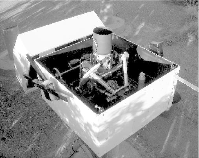
Figure 1: The new generation HAT-5 installed to FLWO: Canon 200 mm f/1.8 lens and Apogee 2K$\times$2K CCD attached to a friction driven horseshoe mount, protected by a clamshell dome.

We were fortunate to acquire by long-term loan the hardware of the de-comissioned ROTSE-I project (Wren et al., 2001; Akerlof et al., 2000). The CCDs were identical to the one we already used, but the Canon 200 mm f/1.8L lenses have a four times larger entrance pupil, and are of much better optical quality than the previously used lens. Many hardware modifications were made, in order to ameliorate difficulties of precise relative photometry over the wide field of view, as described in §2.

The HAT horseshoe mount, an open-loop control system, is friction-driven by stepper motors, without encoders to record the exact position. Our pointing accuracy was improved by re-designing the horseshoe and the declination drive, thus achieving better friction and balance of the telescope. Use of precision rollers for the RA-axis decreased our periodic errors in tracking. We do not use auto-guiding for several reasons: i) it complicates the current, relatively inexpensive hardware setup, ii) our tracking errors in 5 minute exposures are negligible, iii) due to differential refraction, stars in the corners would drift away on a sub-pixel scale even with auto-guiding. However, we are able to perform astrometry immediately after each exposure, and correct the position of the telescope before the next exposure, thus achieving few-pixel pointing precision.

The fast focal ratio lens also involved several modifications. We had to develop a computer-controlled focusing system, driven by a 2-phase stepper motor (§2 W3). The different lens, and longer effective “telescope” length resulted in re-designing the entire dome, and lens-supporting mechanism.

The effects of differential extinction (§2 W5) can be minimized by use of multiple filters, and inclusion of color-terms in the fits of magnitude differences between individual frames. Multiple filters are also essential for quick elimination of some false transiting planet signatures, and for proper standard calibration of the photometry. Because one of the purposes of the HAT instrument is to provide useful data for variability monitoring as well, we decided to use standard Cousins I filter as primary band, complemented by Johnson V (both made following the prescription of Bessell 1990). The 14$\mu$ pixel size, fast focal ratio and short backfocus of the lens (42 mm) pose stringent requirements on the filter exchanger. We designed our own exchanger which is capable of few micron re-positioning accuracy.

4 PSF broadening

The hardware modifications outlined in §3, and the custom-built software (see §6 below) took care of some of complications that arise from wide-field photometry, but not of effects that are related to the undersampled profiles (see §2: F4, U1-5, C1-2). The stellar profiles of HAT-5 are $\sim$1.5 pix, at pixel scale of 14″, showing slight variation over the 8.2°$\times$8.2°FOV. Our suspicion was that broadening the instrumental PSF, so as to achieve better sampling, could improve the photometric precision, which previously was never less than $\sim$1%.

Because we did not have the freedom to change the CCDs to a type with finer pixel-resolution, achieving better sampling required widening the stellar profiles. Our first attempt to do this by generating artificially bad seeing in front of the lens with heating elements failed. Defocusing of the lens enough to broaden the profiles sufficiently did not work, because it introduces strong, spatially dependent distortion of the profiles. Hence we decided to broaden the PSF by stepping the telescope pointing during the exposure.

The resolution of the HAT stepper motors is 1″ in RA (1/15 pix) and 5″ in Dec (1/3 pix), respectively, and any sequence of stepping commands can be generated and superposed on the sidereal-rate tracking from software, using the RealTime Linux drivers. We reprogrammed the high-level image acquisition program so that during the exposure the telescope steps around the central position on a prescribed pattern (Fig. 2).

We experimented with $\sim$25 different broadening-patterns, that is, patterns of pointing offsets from the central pointing position, together with dwell times at each pointing offset. Small movements of the telescope were found not to be completely deterministic, because of missing microsteps and the elasticity of the sprockets, so we perform the stepping pattern a few times (generally 3) during the exposure to avoid asymmetries in the profiles. We also modeled the expected profile by superposing the intrinsic 1.7 pix wide Gaussian profiles on the offset pointing grid with weights corresponding to the time-intervals spent at the grid-points. When composing a wider profile by this superposition, too large-amplitude grid-steps cause a flat-top profile with humps, i.e. the resolution of the grid has to be smaller than the intrinsic FWHM. We require that the superposed profile also be a Gaussian to a very good approximation; only a few of the patterns fulfill this requirement. The best pattern we achieved consisted of stepping during the exposure to positions 10″ and 20″ in a N,E,S,W direction from the center position, and positions 10″ from the center in a NE, SE, SW, and NW direction (see Fig. 2). The resulting PSF is 2.3 pix wide, broadened from the 1.7 pix intrinsic value with no stepping.

Figure 2: The PSF-broadening pattern the telescope executes during an exposure. The amplitude of tiny movements is 10″, which corresponds to 10 microsteps in RA (on the Celestial Equator), and 2 microsteps in Dec. The pattern starts from the center to the South, continues to the N, W, E, and finally ends in the diagonal directions, as indicated by consecutive numbers. The size of dots is proportional to the dwell times spent at that grid-point. The solid-line grid shows the pixel size (14″), the inner concentric circle the FWHM of a typical intrinsic PSF (1.7 pix), and the outer circle the FWHM of the broadened PSF (2.3 pix).

The great advantage of this PSF-broadening approach is that to first order all the stars in the FOV are broadened in the same manner. To second order, because the telescope is moved in the RA-Dec system, stars experience slightly different true angular movements in RA as a function of declination. The ratio of these movements on the top and bottom of the 8.2° field is close to unity, being exactly 1.0 when the field center is at $\delta=0\arcdeg$, and reaches 1.18 at $\delta\approx 50\arcdeg$, although the ratio of resulting profile widths is less. This is approximately our tolerance (defined by being equal to the nightly variation of the PSF in the center of the field we experience due to other reasons), and hence sets a limit on observational declination.

PB not only broadens the profiles, but also smooths out their spatially-dependent distortion, producing profiles that are more homogeneous over the field. Also, while the intrinsic profiles are subject to tracking errors and other impacts (gusts, etc.), the PB ones are more stable in time. This technique yielded far better precision for bright stars in moderately crowded fields with simple aperture photometry than the “tracking” frames, as described in §7. We emphasize that it is not the only way of improving precision for small-telescope projects, but rather a specific practical solution given our restrictions (CCDs, lenses, budget).

5 Observations

HAT-5 started up observations at FLWO in February, 2003. The first month was spent with various experiments, such as fine-tuning the PB patterns. Routine observations started in March, 2003, and the telescope observed on 91 nights until the monsoon arrived (10 July). Although HAT-5 was started up again after the monsoon (in September), now as part of the HAT Network, along with two other telescopes at FLWO, the primary subject of this paper is the data that have been reduced and analyzed from the Spring season of HAT-5.

The typical scenario at each observing session was the following: in the early evening, after cooling down the CCD, bias frames were taken. If the sky was clear, as seen from a live webcamera and satellite images, the telescope was enabled to open up (remotely, over the Internet, typically from the CfA). This is the only point that needed manual interaction with the telescope system; otherwise the entire observing session and the scheduling of tasks was done automatically. The skyflat program started at sunset, and frames were taken at the closest flatfield region to the optimal point on the sky with the smallest gradients (Chromey & Hasselbacher, 1996). The main program was launched by the automatic “virtual observer” program after nautical twilight. We observed two selected regions; one sparse field in the beginning of the night (in the constellation Sextans, centered on $\alpha$ = 10^h00^m00^s, $\delta$ = 00°00′00″, and labeled G416), and a moderately crowded field in the second half of the night (in the constellation Hercules, centered on $\alpha$ = 17^h36^m00^s, $\delta$ = 37°30′00″, and labeled G195). Both fields were observed with 300s exposures, primarily in I-band, and with the PB-pattern that yielded $\sim 2.5$ pix FWHM on average. Unfortunately, due to a slow drift of the instrument adjustments, as well as seasonal thermal expansion, the PSF increased from 2.3 pix (early Spring) to more than 3 pix (June). Occasionally tracking-frames were taken, as well as V-band images. Depending on the length of the night, approx. 80 frames were accumulated per session, with equal number of G416 and G195 frames in the beginning, and almost entirely G195 frames at the end of the Spring season. The maximal zenith angle of the fields was 60°. Immediate post-exposure coordinate corrections (see §3) were not applied; their potential importance was only realized later, when reducing this dataset. During the entire season, we collected 1300 frames for field G416 and 3300 for G195. The morning skyflats were taken in a similar manner to the evening. We closed the session by taking long dark frames and bias exposures. All data were archived to tapes immediately after the session. For comparison of the tracking and PB-patterns, some nights were devoted to experiments, in which frames of the same field were taken in alternating mode. This way we could directly compare the precision of the two methods by looking at the rms of light-curves from tracking and PB light-curves.

6 Data reduction

Image calibration was performed in a standard way, using GNU/Linux shell scripts to control IRAF and self-developed tasks. Each night is dealt with as a separate unit with its own calibration frames, unless some of the calibration observing programs failed (bad weather, no useful skyflat regions, etc.). In these cases, calibration from neighboring nights was used. Standard overscan, bias, dark and flatfield corrections were applied. (The Thomson chip in the AP10 CCD has no true overscan; instead we are using an electronic overscan, which is the read-out of several columns before the image columns.) Inferior quality skyflat frames are rejected using various fits to statistical parameters of all the flats taken during the session (standard deviation vs. mean value, proximity to desired 8000 ADU mean level, etc.). This way the presence of clouds in the skyflats can also be detected, in case they were not checked or realized on the web camera. The images are also subject to quality filtering before beginning the astrometry and photometry, using mean level, standard deviation of the background, profile widths, etc.

Astrometry

We used fixed-center aperture photometry to derive instrumental magnitudes. The central X,Y positions of the sources on any frame are those of an astrometry reference frame (AR) transformed to the individual frame. The AR is chosen to be a tracking frame, where profiles are sharp, and merging of the sources is less severe than on PB images. (Note, therefore, that the full implementation of the PB technique requires the acquisition of both tracking and PB-frames.) A grid of $\sim$2000 stars is used on the AR and individual frames to determine the geometric transformation between the frames. We start by triangle matching the frame to the AR grid, and after a linear transformation is established, we increase the rank of the fit, and tune the sigma clipping, until we reach a satisfactory 4th order fit with rms of residuals smaller than 0.1 pix. This iterative procedure is designed to work in a more general application of matching frames with a star catalogue, and is more complicated than necessary for simply matching frames to each other, but was used for convenience. General triangle matching is extremely CPU-intensive ($\propto N^{9/2}$, where N is the number of stars), because a great many ($\approx N^{3}/6$) triangles are generated and have to be paired (Groth, 1986). Furthermore, in this case the larger triangles can be significantly distorted with such a fast focal ratio imaging. So instead, we generate a mesh of local triangles with an optimized algorithm, using Delaunay-triangulation (e.g. Shewchuk, 1996), and use these local triangles (only N-2 per frame) for finding the initial transformation. The computation with Delaunay-triangulation scales only as $N^{p}$, where $2<p<3$. While Delaunay-triangulation is a more special case than general triangle-matching algorithms (because it requires similar surface density of the two datasets to be matched, so that the local triangles generated have a common subset), in our case matching the frames to each other always works, except for frames with defects. The same holds for matching frames with the Guide Star Catalogue (Lasker et al., 1990).

Photometry

Fixed center aperture photometry was performed on all the PB frames using the centers we got from transforming a “modified” AR coordinate list to each frame. This modified AR was derived by first selecting one PB frame as the photometric reference (PR) from a dark, photometric night. Then the transformed coordinates of the brightest, non-saturated stars that were missing from the AR (because they saturated on the tracked frames) were appended to it.

The instrumental magnitudes vary between the frames for a number of reasons. First, the extinction changes from night to night, with zenith angle, or with variable photometric conditions. Second, the profile widths also vary, changing not only the accumulated flux in the fixed aperture but also the merging with neighboring sources (§2: M2). Depending on accuracy of field-positioning (“minor” or “major”; see §7), the different placement of the star also causes magnitude offsets (“minor”: F2, F4, U1-2, C1-2; “major”: these plus W2 and F1). To correct for these and possibly other factors, we fitted the magnitude differences from the reference PR frame of the brightest thousand stars as a function of X,Y coordinates in an iterative way with 3 sigma outlier rejection, so as to eliminate variable sources from the magnitude fits. Color-dependence was not incorporated in the fits. The residual of the fits (to fourth order in X and Y) can be as low as 3 millimag, and was typically better than 6 mmag. For non-photometric nights the fit rms was significantly worse than 1%; these large rms values may be used as a criterion to reject such nights. All parameters of the fit were recorded, and later used for quality filtering the data-points.

Based upon the rms of the magnitude fits, approximately 20 of the best frames from the same night as the astrometry reference frame AR were selected, and the transformed magnitude data were averaged (for each star) with weights being the rms values of the fits. This resulting master photometry reference (MR) file was then used for re-fitting all the magnitude files to the MR. This final step reduced our fitting rms to 2 mmag for the best frames, and in general by a factor of 30%.

7 Attainable precision

We derive the photometric precision of the system by looking at the rms variation of light-curves of stars we believe are constant. These are difficult to select a priori, but it is a good assumption that majority of the stars are not variable above the millimagnitude level, and thus we can characterize the photometric precision by the median of the rms of the magnitude variations within a domain of parameters on which photometric precision depends. The principal parameter is the magnitude of the sources, but a magnitude vs. rms plot with wide-field instruments yields a somewhat broader distribution of points, due to the dependence of rms on other parameters, such as radial distance from the field center (due to vignetting). Both observational rms variations and intrinsic stellar variability depend on the timescale of our investigation; we distinguish between nightly, and long-term precision. The latter is typically inferior to the former, because it is affected by instrumental drifts, seasonal variations of the weather, inclusion of non-photometric nights, and long-term variability of some of the stars. Photometric precision also depends on the time-resolution of the data. Binning of course will reduce the rms of the light-curve to the extent that the error of individual data points is random rather than systematic. The following discussion assumes the 5-min time-resolution of HAT observations, unless noted otherwise. It is worth noting that while the signal-to-noise ratio (SNR) of a planetary transit detection is basically unaffected by binning, the higher precision of binned data points can be useful in confirming the reality of the transit.

Comparison of precision with tracking and PSF-broadened frames was established on photometric nights by taking alternating 5min exposures of the same field with the two methods. Although this paper deals mainly with HAT-5, we also present the results of the same experiment performed simultaneously to HAT-5 on a different stellar field with the essentially identical HAT-6 telescope, located at the same site. This way we can rule out possible detector-related issues, and because the gain by PB is greater for HAT-6, it makes a useful comparison. The difference between HAT-5 and HAT-6 lies in the intrinsic profile widths: for HAT-5 this width is 1.7 pix, strongly variable over the field, while for HAT-6 the PSF is 1.2 pix wide. (This is probably due to the differences between the seemingly identical lenses.) The PSF-broadening widens the profiles to 2.3 pix on HAT-5, and to 2.0 pix on HAT-6. Light-curves were constructed from both series (tracking and PB) of images, and the I-magnitude vs. rms curves were compared. Naturally, due to the different PSF-widths with tracking and PB, the optimal parameters (aperture, sky annulus) for photometry were different, so we compare the best photometry we could achieve with the given technique. Tracking and PB aperture photometry results were transformed to the same instrumental system using $\sim 1000$ stars, with rms of the transformation smaller than 0.01mag, so that both sets of data are plotted on the same magnitude scale. Following this, we performed crude absolute calibration to I-band, using $\sim$ 20 non-saturated Hipparcos (Perryman et al., 1997) stars in each field. The rms of these transformations is surprisingly high: $\sim 0.2$ mag for each field, although this does not affect our conclusions when comparing PB to tracking, which are very precisely in the same instrumental system.

Fig. 4 compares the precision attainable when employing straight tracking or PB. For both HAT-5 and HAT-6, the precision on the bright end is considerably better with PB (grayscale open circles) than with tracking (median value only shown as thick solid lines, to avoid confusion of overlapping individual points). However the precision using PB is worse for faint stars. The poorer behavior on the faint end can be explained by the effect of increased sky-background noise under the widened profile of stars with small flux. The dramatic improvement in precision on the bright end is especially significant for HAT-6 (right), which has sharper intrinsic profiles. (The fact that stars extend to brighter magnitudes at HAT-5 is due only to the technical detail that the AR used for HAT-5 data reduction of these test observations was established on frames with wider intrinsic PSF, thus containing brighter non-saturated coordinates for fixed-center photometry. Saturated sources, because of the coordinate uncertainties of their profiles, were rejected from the coordinate lists in this comparison.) It may be noted that the above-mentioned rms uncertainty of $\sim 0.2$ mag in the transformation from instrumental to true I-band magnitudes means that the vertical axes of the left and right panels of Fig. 4 must be considered uncertain relative to each other by perhaps as much as 0.1 mag.

The gain in precision when PB is used can be attributed to a number of causes: The residual inter-pixel variations of imperfect flatfielding (and to smaller extent, the intra-pixel variations) are somewhat smoothed out by the broader PSFs. Because of the broader PSF, and use of brighter non-saturated stars with higher S/N, the resulting magnitude transformation between the frames is more accurate. Because the optimal aperture for PB is wider, the errors in the centroid position of stars yield smaller errors in photometry. Finally, the more homogeneous profiles with time and position within the field act to maintain the stability of the measured magnitudes over pointing changes or focus changes; at the same time the magnitude transformation is simpler than for tracking frames.

Theoretical expectations on the noise sources are also shown on Fig. 4 (thin solid lines), using the standard formulae described in e.g. Newberry (1991) that depend on the incoming flux (in $e^{-}$), gain of the CCD, number of pixels in the aperture and background annulus, and the standard deviation of the background (as measured from reduced frames). It may be seen that the theoretical curves describe the empirical results of PB fairly well, but with the undersampled (pure tracking) profiles other effects start to dominate, and the measured rms values (median showed as thick solid lines) diverge from the theory: they flatten on the bright end, at values (0.5% for HAT-5 and greater than 1% for HAT-6) that depend on the width of the intrinsic PSF.

In summary, while precision in the star-noise limited regime is drastically improved, the precision becomes a steeper function of magnitude, and degrades rapidly for faint sources in the sky-noise limited regime. The actual performance depends on the intrinsic and broadened PSF widths. The PB-technique provides another degree of freedom when optimizing the photometric characteristics of a system. The advantages are determined by the goals; if the purpose is to optimize precision for faint sources (even at the cost of losing precision for bright stars) or to improve detection of larger amplitude variability for very faint sources (as was the case for the previous use of these detectors and lenses in the ROTSE-I project, Akerlof et al. 2000), then the sharpest possible profiles are desired. PSF-broadening is not a general solution for improving precision of a system, rather a special technique tested on our instrumentation, which increases the number of stars having photometry better than 1%, and thus the chance of detecting planet transits. For wide-field planet searches such as ours, which use semi-professional, front-illuminated CCDs, if precision for bright stars flattens at an undesired $\sim 1\%$ value, PB might be a workaround.

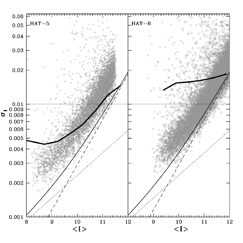
Figure 4: Photometric precision attained with HAT-5 (left panel) and HAT-6 (right), as established from the rms of the light-curves with 5min time-resolution, after 3 sigma rejection of outlier points. The thick solid line represents the median rms values in 0.25mag bins from simple tracking frames, while the open circles show the improvement by PB for each star, reaching 2 mmag for the brightest stars. The difference is enhanced at HAT-6, where the intrinsic PSF is very sharp (1.2 pix) compared to the PB (2.0). Theoretical noise estimates are also given for the PB-case (3.0 pix aperture): the combined noise (thin solid line) is the sum of sky-noise (dashed line) and photon-noise (dotted line).

7.1 Long-term variation of precision

Over the 4 months of operation in the 2003 Spring season, we experienced a long-term degradation of the nightly precision, as is shown in Fig. 5, where we plot the nightly rms variations of stars of similar brightness ($I=10\pm 0.25$, $\sim$600 sources) as a function of JD (big filled boxes). This was later found to be due to the PSFs becoming increasingly “over-broadened”, because of a tight declination-drive sprocket on HAT-5, and possibly other instrumental misalignments. The outlier points are due to non-photometric nights. The rms of the magnitude transformation to the photometric reference is also plotted for each frame (small dots, $\sim$80 per night), and its correlation with the actual nightly rms of stars can be used as a direct measure of the photometric conditions. We stress that the data reduction methodology discussed earlier ensures that the stability of magnitudes over several months is comparable to the rms of magnitude-fits from individual frames to our photometric reference.

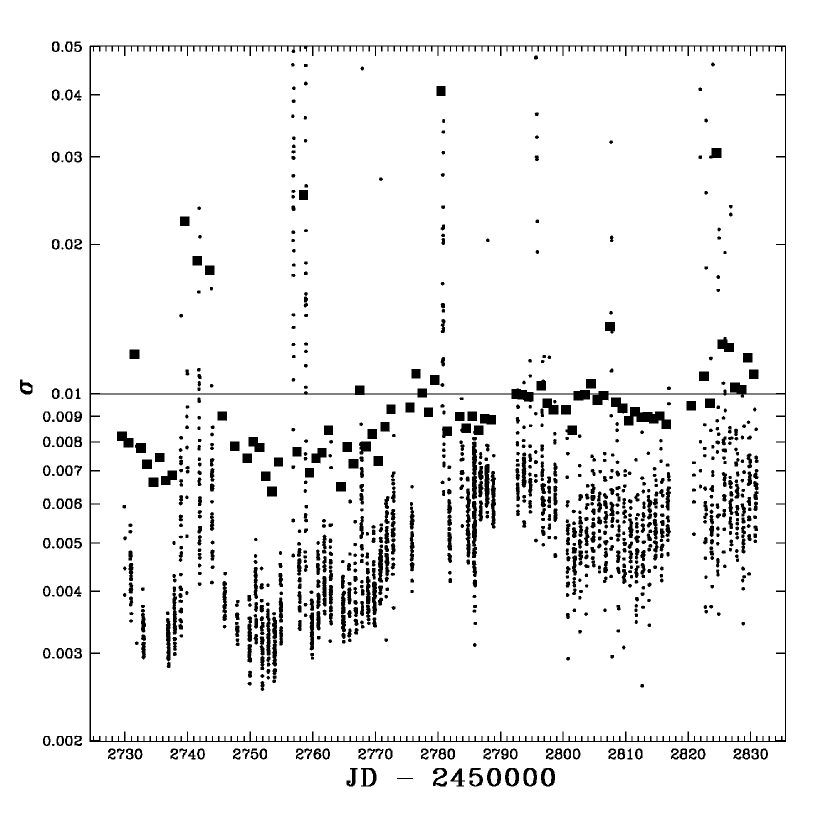
Figure 5: Long term photometric precision of HAT-5 in the Spring 2003 season, as a function of Julian date. Both the nightly rms variations of $I=10\pm 0.25$ magnitude stars (big filled boxes) and the rms of the magnitude transformation to the reference for each frame (small dots) are plotted. Beside the outlier points due to non-photometric nights, a long-term degradation is also visible.

Fourier analysis of the brightest 2000 light-curves (with rms typically less than 1%) revealed other effects, which potentially harm planet and low-amplitude variability detection capabilities. These are miscellaneous low-amplitude ($\sim 1\%$, always smaller than 0.1mag) systematic variations exhibited by most of the stars, the exact subset of stars depending on the effect itself. The fact that the variations are not intrinsic to the stars is seen from either the frequency: daily variations close to 1, 1/2 and 1/3 $d^{-1}$, or by peaks in the frequency-distribution histogram: 38min and 80min modulations. Although we have indications about the origin of these systematics, they haven’t been completely understood and elimination poses a serious task to be solved. Some are definitely related to the minor pointing imperfections of the telescope, such as periodic tracking errors (with 38min periodicity), and are expected to diminish with the introduction of the position auto-correction technique described in §3 (in use since the Fall of 2003). It is especially intriguing to note that some stars show a daily variation, while others have stable light-curves, and yet for the stars showing this variation no clear dependence on other parameters (color, position) have been found. The various modulations seem to be related, since pre-whitening with the 1 day periodicity usually causes the 80min component almost to disappear. We note that various systematics are also observable in other large scale surveys, such as MACHO (Alcock et al., 2000) and OGLE (Kruszewski & Semeniuk, 2003).

8 Early results

Search for planetary transits

To search for possible planetary transits, a BLS period search (Kovács, Zucker, & Mazeh, 2002) was performed on the moderately rich Hercules field, which had $\sim 3000$ observations, more than the twice the number of observations of the sparse Sextans field. The search was limited to the [0.02,0.98]$d^{-1}$ frequency range with 20000 frequency steps, 200 phase bins, fractional transit lengths of $q_{min}=0.005$ and $q_{max}=0.05$. The BLS spectra generally displayed an increasing background power toward lower frequencies, most probably because of slight long-term systematic trends of the light-curves. Therefore, we fitted 4th order polynomials to the spectra by using 5 sigma clipping so as to minimize the effect of large peaks. Then, these polynomials were subtracted from the spectra and the residuals were examined for outstanding peaks. The BLS algorithm, similarly to other matching methods, creates subharmonics, and the 1day systematic variation of certain stars resulted in false frequency peaks at k/n [$d^{-1}$], where k and n are small integers. The distribution function of the peak BLS frequencies clearly showed such peaks, and stars exhibiting these periodicities were excluded.

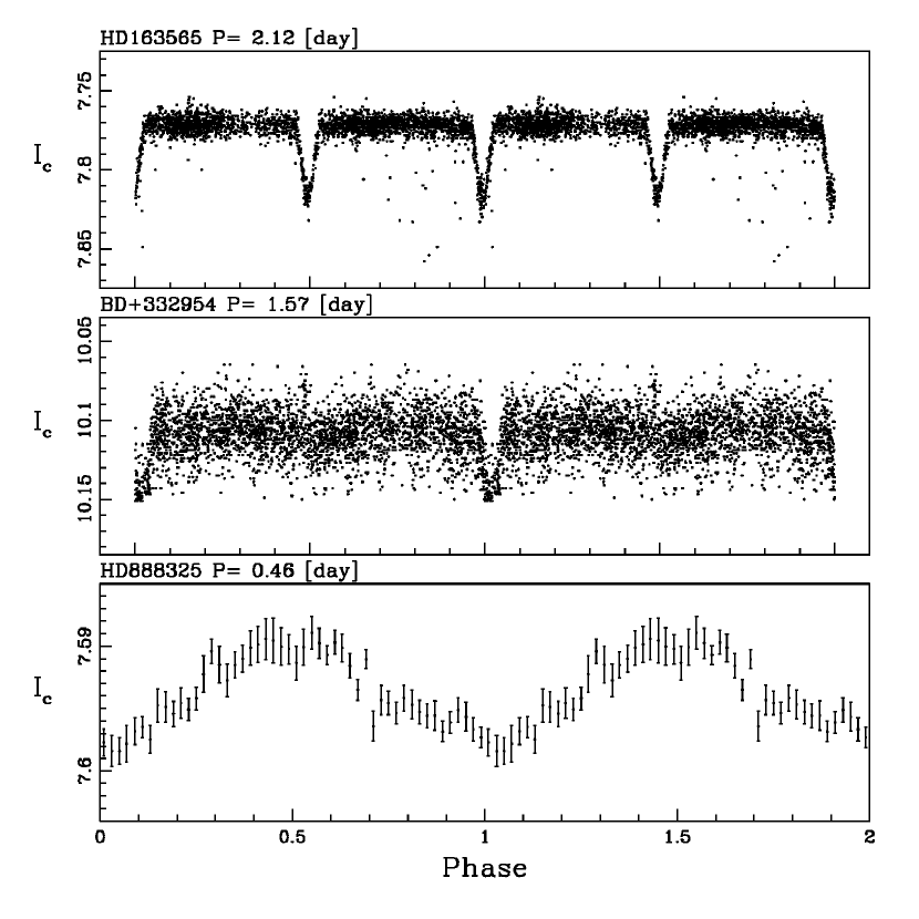
Figure 6: Phased light-curves of three variables of special interest. Upper panel: Star HD 163565 shows V-shaped photometric dips of 4% depth, characteristic of grazing eclipses, with full period (two nearly identical dips) of 2.11 days. Middle panel: Star BD+33 2954 with F8 spectrum shows a periodic dip with amplitude of only 0.032 mag, period 1.57 days, and duration 2.0 hrs, perhaps caused by an M-dwarf; there may be a blended tertiary in the system. Lower panel: HD 88832 is an A5 star with only 8 mmag peak-to-peak amplitude of variation. The light-curve for this star has been binned in phase with $\sim 25$ data points occurring in each bin.

Finally, a sample of 133 stars was selected from the remaining sources, having BLS spectral peaks with signal-to-noise ratio (SNR) greater than 6.0. Visual inspection of the folded light-curves further narrowed the sample to 23 variables, with most detections being marginal. The bottom line is that no definite planetary transit detections have been found in this early dataset. The two best cases (Figure 6 upper and middle panel) belong to a V-shaped grazing eclipse of 4% depth observed for the A0 star HD 163565, and a shallow (3.5%) eclipse of the F8 star BD+33 2954, which is too deep to be planetary transit; the system also shows a low-amplitude sinusoidal variation in its high-luminosity state. The remaining sources were well below the significance of the the above two stars.

We also performed tests on the detectability of periodic transit events on the Hercules field. The present figures for the detection rates are preliminary, as the technique for recovering signals is under development. A transit of P=$5.12345^{d}$, dip=$-0.015$ mag, length = $0.03P$ was added to the brightest $\sim 2000$ observed light-curves ($I\lesssim 10.5$). This way the recovery was tested on the real observations, not even excluding sources that show variability (the fraction of the latter is approx. 10% or less, see later). The BLS test was run on the time-series with search parameters described in the beginning of this section. The selection criterion for detection were i) SNR of the BLS spectrum greater than 6.0, and ii) period corresponding to the peak in the range of [5.102,5.154] days. The detection rate is rather high (74%) on the bright end, especially after excluding variable stars from the sample (82%). However, it drops to 29% for the faintest stars at $I\approx 10.5$.

General Stellar Variability

The few-mmag precision of HAT for bright stars allows for investigating general stellar variability at levels not normally attainable from the ground with small, very wide-field telescopes. HAT’s capability to measure thousands of stars in a single field with better than 1% precision should enable it to contribute significantly to general stellar variability studies.

For strictly periodic variations, phase-binning of observations over many periods allows us to achieve relative precision in a light-curve far better than that of individual observations; the ultimate limit is placed by systematic effects that cannot be corrected for. As an example of phase-binning, Figure 6 (lower panel) illustrates a very low-amplitude (8 mmag peak-to-peak) quasi-sinusoidal photometric variation of HD 88832, an I=7.6 (V=8.1) A5 star in the Sextans field. Analysis of Variance (AoV: Schwarzenberg-Czerny, 1996) study revealed a predominant photometric period of 0.462 days. The data (1226 data points over 65 days) were phased to this period and divided into 50 bins, so that approximately 24 data points occur in each. The average standard deviation of the mean of these data points is 1.1 mmag, illustrating that the magnitude calibration is stable at that level over a period of at least two months.

We note that for detection of a planetary transit, the situation is much less favorable, since a typical transit would occupy only about 3 to 4 percent of the total phase diagram (i.e. one to two of the phase bins in Figure 6 lower panel).

In order to establish a preliminary variable star inventory, light-curves were searched for using Discrete Fourier Transformation (DFT) with 5-sigma clipping of potentially bad data-points, and imposing a minimal SNR of 6.0. Variables with close integer frequencies were rejected ($f_{0}<0.02d^{-1}$ and $n-0.018<f_{0}<n+0.018d^{-1}$ where n is integer). Finally, folded light-curves were subject to visual inspection and rejection. This preliminary analysis definitely lost low-amplitude variables hidden in the systematic trends, or those with multiple periods, and it is also incomplete at long periods that are comparable to the time-span of observations. Nevertheless, most variables with greater than 0.01mag amplitude were recovered, and the total number turned out to be $\sim 220$ (11%) in the Hercules field, and $\sim 110$ (5.5%) in the Sextans field, respectively, out of the 2000 brightest stars tested. This difference is partly because of the smaller number of observations for the Sextans field (1300 vs. 3300), but might also be credited to different stellar populations tested.

9 Summary and future prospects

Photometric precision substantially better than 1% is important for detection of giant planets transiting sun-like stars, and also can contribute significantly to general stellar variability research. We have discussed the difficulties in attaining this level of precision when using an instrument such as HAT, i.e. using a lens with a fast focal ratio and wide field, attached to a front-illuminated CCD. Most of these difficulties can be dealt with by careful design of the instrumentation, specialized observing techniques, and custom-written software. The problem of under-sampling of stars needs special treatment. We described our PSF-broadening technique which greatly improved the precision, reaching 2 mmag rms for stars at $I\approx 8$. We attribute the gain in precision to the smoothing of residual inter- and intra-pixel variations caused by imperfect short-scale flatfielding, the use of brighter stars for matching the magnitude system of frames, and the better behavior of existing photometry software on broader PSFs.

HAT-5 has been operational since early Spring, 2003, and the initial few months were devoted for tests. Based on the observations spanning four months, 91 nights in total, we determined the long-term precision and investigated low-amplitude systematic variations. Our search for periodic transits, performed on both of our observed fields, has not yielded any definite detection of planetary transits. A few shallow transits and grazing eclipsing binaries were revealed, along with several hundred variable stars.

In order to increase the chance of detecting transiting planets, a network of HAT telescopes (HATnet) has been developed following the installation of our prototype HAT-5. Two additional systems, essentially identical to HAT-5 (HAT-6 and HAT-7) were installed at FLWO, and have been operational since September, 2003. Two more, also identical, HAT telescopes have now been installed at SAO’s Submillimeter Array site on Mauna Kea, Hawaii, and have been observing since November, 2003. A great advantage of the HATnet, presently consisting of five stations, is that the instruments have nominally identical telescope mounts, software environment, lenses and CCDs. The longitude separation of 3 hours between FLWO and Hawaii, and uncorrelated weather patterns significantly extend our time coverage of fields. We hope that continuous operation of HATnet and further improvements to be introduced in our data reduction and analysis software system will further enhance our ability of transit detection and to study low-amplitude stellar variability in general.

References

- Akerlof et al. (2000) Akerlof, C. et al. 2000, ApJ, 532, L25
- Alcock et al. (2000) Alcock, C. et al. 2000, ApJ, 542, 257
- Bakos et al. (2002) Bakos, G. Á., Lázár, J., Papp, I., Sári, P., & Green, E. M. 2002, PASP, 114, 974
- Bessell (1990) Bessell, M. S. 1990, PASP, 102, 1181
- Brown et al. (2001) Brown, T. M., Charbonneau, D., Gilliland, R. L., Noyes, R. W., & Burrows, A. 2001, ApJ, 552, 699
- Brown (2003) Brown, T. M. 2003, ApJ, 593, L125
- Buffington, Booth, & Hudson (1991) Buffington, A., Booth, C. H., & Hudson, H. S. 1991, PASP, 103, 685.
- Charbonneau et al. (2000) Charbonneau, D., Brown, T. M., Latham, D. W., & Mayor, M. 2000, ApJ, 529, L45
- Charbonneau et al. (2002) Charbonneau, D., Brown, T. M., Noyes, R. W., & Gilliland, R. L. 2002, ApJ, 568, 377
- Chromey & Hasselbacher (1996) Chromey, F. R. & Hasselbacher, D. A. 1996, PASP, 108, 944.
- Groth (1986) Groth, E. J. 1986, AJ, 91, 1244
- Henry et al. (2000) Henry, G. W., Marcy, G. W., Butler, R. P., & Vogt, S. S. 2000, ApJ, 529, L41
- Horne (2003) Horne, K. 2003, ASP Conf. Ser. 294: Scientific Frontiers in Research on Extrasolar Planets, eds. D. Deming and S. Seager, San Francisco, The Astronomical Society of the Pacific, 361
- Konacki et al. (2003) Konacki, M., Torres, G., Jha, S., & Sasselov, D. D. 2003, Nature, 421, 507
- Kovács, Zucker, & Mazeh (2002) Kovács, G., Zucker, S., & Mazeh, T. 2002, A&A, 391, 369
- Kruszewski & Semeniuk (2003) Kruszewski, A. & Semeniuk, I. 2003, Acta Astronomica, 53, 241
- Landolt (1992) Landolt, A. U. 1992, AJ, 104, 340
- Lasker et al. (1990) Lasker, B. M., Sturch, C. R., McLean, B. J., Russell, J. L., Jenkner, H., & Shara, M. M. 1990, AJ, 99, 2019.
- Newberry (1991) Newberry, M. V. 1991, PASP, 103, 122
- Perryman et al. (1997) Perryman, M. A. C. et al. 1997, The Hipparcos and Tycho Catalogues, ESA SP-1200, Vol. 1-17
- Pojmański (1997) Pojmański, G. 1997, Acta Astronomica, 47, 467.
- Queloz et al. (2000) Queloz, D., Eggenberger, A., Mayor, M., Perrier, C., Beuzit, J. L., Naef, D., Sivan, J. P., & Udry, S. 2000, A&A, 359, L13
- Schwarzenberg-Czerny (1996) Schwarzenberg-Czerny, A. 1996, ApJ, 460, L107
- Shewchuk (1996) Shewchuk, R. J. 1996, in Applied Computational Geometry: Towards Geometric Engineering, eds. M. C. Lin and D. Manocha, Berlin, Springer-Verlag, vol. 1148, 203, http://www-2.cs.cmu.edu/~quake/triangle.research.html and references therein
- Torres et al. (2003) Torres, G., Konacki,D. M., Sasselov, D. D. & Jha, S. 2003, astro-ph 0310114, submitted to ApJ
- Udalski et al. (2002) Udalski, A., Zebrun, K., Szymanski, M., Kubiak, M., Soszynski, I., Szewczyk, O., Wyrzykowski, L., & Pietrzynski, G. 2002, Acta Astronomica, 52, 115
- Vidal-Madjar et al. (2003) Vidal-Madjar, A., Lecavelier des Etangs, A., Désert, J.-M., Ballester, G. E., Ferlet, R., Hébrard, G., & Mayor, M. 2003, Nature, 422, 143
- Wren et al. (2001) Wren, J. et al. 2001, ApJ, 557, L97