Pacman (II): Application and Statistical Characterisation of Improved RM Maps

Abstract

We proposed a new method – Pacman – to calculate Faraday rotation measure (RM) maps from multi-frequency polarisation angle data (Dolag et al.) in order to avoid the so-called $n\pi$-ambiguity. Here, we apply our Pacman algorithm to two polarisation data sets of extended radio sources in the Abell 2255 and the Hydra A cluster, and compare the RM maps obtained using Pacman to RM maps obtained employing already existing methods. Thereby, we provide a new high quality RM map of the Hydra north lobe which is in a good agreement with the existing one but find significant differences in the case of the south lobe of Hydra A. We demonstrate the reliability and the robustness of Pacman. In order to study the influence of map making artefacts, which are imprinted by wrong solutions to the $n\pi$-ambiguities, and of the error treatment of the data, we calculated and compared magnetic field power spectra from various RM maps. The power spectra were derived using the method recently proposed by Enßlin & Vogt (2003). We demonstrate the sensitivity of statistical analysis to artefacts and noise in the RM maps and thus, we demonstrate the importance of an unambiguous determination of RM maps and an understanding of the nature of the noise in the data. We introduce and perform statistical tests to estimate the quality of the derived RM maps, which demonstrate the quality improvements due to Pacman .

1 Introduction

Magnetic fields are ubiquitous throughout the universe. One method to study them is the analysis of the Faraday rotation effect. This effect describes that if polarised radiation traverses a magnetised plasma the plane of polarisation of the radiation is rotated. The change in polarisation angle is proportional to the squared wavelength $\lambda^{2}$. The proportionality constant is called rotation measure (RM). Various methods have been proposed in order to calculate RM maps from multi-frequency polarisation data sets (e.g. Vallée & Kronberg, 1975; Haves, 1975; Ruzmaikin & Sokoloff, 1979; Sarala & Jain, 2001). The difficulty involved in this calculation arises from the fact that observations constrain the polarisation angle $\varphi$ only up to additions of $\pm n\pi$. This leads to the so-called $n\pi$-ambiguity.

In a previous paper (Dolag et al., 2003, hereafter Paper I), we proposed a new approach for the unambiguous determination of RM and of the intrinsic polarisation angle $\varphi^{0}$ at the observed, polarised radio source from multi-frequency polarisation data sets. The proposed algorithm uses a global scheme in order to solve the $n\pi$-ambiguity. It assumes that if regions exhibit small polarisation angle gradients between neighbouring pixels in all observed frequencies simultaneously then these pixels can be considered as connected. Information about one pixel can be used for neighbouring ones and especially the solution to the $n\pi$-ambiguity should be the same.

Faraday rotation measure maps are analysed in order to get insight into the properties of the RM producing magnetic fields such as field strengths and correlation lengths. Artefacts in RM maps which result from $n\pi$-ambiguities can lead to misinterpretation of the data. Recently, Enßlin & Vogt (2003) proposed a method to calculate magnetic power spectra from RM maps and to estimate magnetic field properties. They successfully applied their method to RM maps (Vogt & Enßlin, 2003) and realised that map making artefacts and small scale pixel noise have a tremendous influence on the shape of the magnetic power spectra on large Fourier scales – small real space scales. Thus, for the application of these kind of statistical methods it is desirable to produce unambiguous RM maps with as little noise as possible. This and similar applications are our motivations for designing Pacman (Paper I) and to quantify its performance (this Paper).

In order to detect and to estimate the correlated noise level in RM and $\varphi^{0}$ maps, Enßlin et al. (2003) recently proposed a gradient vector product statistic. It compares RM gradients and intrinsic polarisation angle gradients and aims to detect correlated fluctuations on small scales, since RM and $\varphi^{0}$ are both derived from the same set of polarisation angle maps.

In Paper I, we describe in detail the idea and the implementation of the Pacman algorithm. Furthermore, we presented a test of the algorithm on artificially generated maps where we demonstrated that Pacman yields the right solution to the $n\pi$-ambiguity. Here, we want to apply this algorithm to polarisation observation data sets of two extended polarised radio sources located in the Abell 2255 (Govoni et al., 2002) cluster and the Hydra cluster (Taylor & Perley, 1993). This is described in Sect. 3. Using these polarisation data, we demonstrate the stability of our Pacman algorithm and compare RM maps obtained from a standard fit algorithm. A “standard fit” algorithm is considered to be the algorithm which performs a pixel by pixel least squares fit using the methods suggested by Vallée & Kronberg (1975); Haves (1975); Ruzmaikin & Sokoloff (1979).

We demonstrate the importance of the unambiguous determination of RMs for a statistical analysis by applying the statistical approach developed by Enßlin & Vogt (2003) to the RM maps in order to derive the power spectra and strength of the magnetic fields in the intra-cluster medium. We also discuss the influence of error treatment in the analysis. The philosophy of this statistical analysis and the calculation of the power spectra is briefly outlined in Sect. 2.3 whereas the results of the application to the RM maps are presented in Sect. 3.

In addition, we apply the gradient vector product statistic V as proposed by Enßlin et al. (2003) in order to detect map making artefacts and correlated noise. The concept of this statistic is briefly explained in Sect. 2.1 and in Sect. 3, it is applied to the data. After the discussion of our results, we give our conclusions and lessons learned from the data during the course of this work in Sect. 4.

Throughout the rest of the paper, we assume a Hubble constant of H${}_{0}=70$ km s^-1 Mpc^-1, $\Omega_{m}=0.3$ and $\Omega_{\Lambda}=0.7$ in a flat universe. The notation used follows Paper I.

2 Statistical Analysis of RM maps

2.1 Gradient Vector Product Statistic

Enßlin et al. (2003) introduced a gradient vector product statistic V to reveal correlated noise in the data. Observed RM and $\varphi^{0}$ maps will always have some correlated fluctuations on small scales, since they are both calculated from the same set of polarisation angle maps, leading to correlated fluctuation in both maps. The noise correlation between $\varphi^{0}$ and RM errors is an anti-correlation of linear shape and can be detected by comparing the gradients of these quantities. A suitable quantity to detect correlated noise between $\varphi^{0}$ and RM is therefore

$$V=\frac{\int d^{2}x\,\mn@boldsymbol{\nabla}{\rm RM}(\mn@boldsymbol{x})\cdot\mn@boldsymbol{\nabla}\varphi^{0}(\mn@boldsymbol{x})}{\int d^{2}x\,|\mn@boldsymbol{\nabla}{\rm RM}(\mn@boldsymbol{x})||\mn@boldsymbol{\nabla}\varphi^{0}(\mn@boldsymbol{x})|},$$ (1)

where $\mn@boldsymbol{\nabla}{\rm RM}(\mn@boldsymbol{x})$ and $\mn@boldsymbol{\nabla}\varphi^{0}(\mn@boldsymbol{x})$ are the gradients of RM and $\varphi^{0}$. A map pair, which was constructed from a set of independent random polarisation angle maps $\varphi(k)$, will give a $V\ga-1$. A map pair without any correlated noise will give a $V\approx 0$. Hence, the statistic V is suitable to detect especially correlated small scale pixel noise.

The denominator in Eq. (1) is the normalisation and enables the comparison of V for RM maps of different sources, since $V$ is proportional to the fraction of gradients which are artefacts. Since, we especially want to compare the quality between maps of the same source calculated using the two different algorithms, it is useful to introduce the unnormalised quantity

$$\tilde{V}=\int d^{2}x\,\mn@boldsymbol{\nabla}{\rm RM}(\mn@boldsymbol{x})\cdot\mn@boldsymbol{\nabla}\varphi^{0}(\mn@boldsymbol{x}).$$ (2)

The quantity $\tilde{V}$ gives the absolute measure of correlation between the gradient alignments of RM and $\varphi^{0}$. The smaller this value is the smaller is the total level of correlated noise in the maps.

2.2 Error Under or Over Estimation

One problem, we were faced with during the course of our statistical analysis is the possibility that the measurement errors are under or overestimated. Such a hypothesis can be tested by performing a reduced $\chi^{2}_{\nu}$ test which is considered to be a measure for the goodness of each least squares fit and calculates as follows

$$\chi^{2}_{\nu_{ij}}=\frac{1}{\nu}\sum_{k=1}^{f}\frac{\left[\varphi_{{\rm{obs}}_{ij}}(k)-({\rm RM}_{ij}\,\lambda_{k}^{2}+\varphi_{ij}^{0})\right]^{2}}{\sigma_{k_{ij}}^{2}}=\frac{s_{ij}^{2}}{\langle\sigma_{k_{ij}}\rangle_{k}},$$ (3)

where $\nu=f-n_{c}$ is the number of degrees of freedom and $f$ is the number of frequencies used and $n_{c}$ is the number of model parameters in our case, $n_{c}=2$. The parameter $s^{2}$ is the variance of the fit and $\langle\sigma_{k_{ij}}\rangle_{k}$ is the weighted average of the individual variances:

$$\langle\sigma_{k_{ij}}\rangle_{k}=\left[\frac{1}{f}\sum_{k=1}^{f}\frac{1}{\sigma_{k_{ij}}^{2}}\right]^{-1}$$ (4)

If one believes in the assumption of Gaussian noise, that the data are not corrupted and that the linear fit is an appropriate model then any statistical deviation from unity of the map average $\overline{\chi}^{2}_{\nu}$ of this value indicates an under or over error estimation. For a $\overline{\chi}_{\nu}^{2}>1$, the errors have been underestimated and for a $\overline{\chi}_{\nu}^{2}<1$, they have been overestimated.

Unfortunately this analysis does not reveal in its simple form at which frequency the errors might be under or overestimated. However, one can test for the influence of single frequencies by leaving out the appropriate frequency for the calculation of the RM map and comparing the resulting $\chi^{2}_{\nu_{ij}}$ values with the original one.

It is advisable to evaluate the $\chi^{2}_{\nu_{ij}}$-maps in order to locate regions of too high or too low values for $\chi^{2}_{\nu}$ by eye.

2.3 Magnetic Power Spectra

Our Pacman algorithm is especially useful for the determination of RM maps of extended radio sources. RM maps of extended radio sources are frequently analysed in terms of correlation length and the RM producing magnetic field strength. One analysis relying on statistical methods in order to derive magnetic field power spectra was recently developed by Enßlin & Vogt (2003). They successfully applied their method to existing RM maps of radio sources located in Abell 2634, Abell 400 and Hydra A (Vogt & Enßlin, 2003). In the course of their work, they realised that their method is sensitive to map making artefacts and pixel noise, which can lead to misinterpretation of the data at hand. Therefore this method is a good opportunity to study the influences of noise and artifacts on the resulting power spectra.

The observational nature of the data is taken into account by introducing a window function, which can be interpreted as the sampling volume. Especially, a noise reducing data weighting scheme can be introduced to account for observational noise. One reasonable choice of weighting is to introduce a factor $\sigma_{0}^{{\rm RM}}/\sigma^{{\rm RM}}_{ij}$, which we call simple window weighting. Another possible weighting scheme is a thresholding scheme described by $1/(1+\sigma_{0}^{{\rm RM}}/\sigma^{{\rm RM}}_{ij})$, which means that the noise below a certain threshold $\sigma_{0}^{{\rm RM}}$ is acceptable and areas of higher noise are down-weighted.

Note, that magnetic power spectra, which are calculated using the approach explained above, are used as valuable estimator for magnetic field strengths and correlation lengths. However, since the spectra are shaped by and are very sensitive to small scale noise and map making artefacts, we use them here to quantify the influence of noise and artefacts rather than as an estimator for characteristic properties of the RM producing magnetic fields.

3 Application to data

For the calculation of what we call further on the standard fit RM maps, we used the $\chi^{2}$ method suggested by Vallée & Kronberg (1975) and Haves (1975). Also for the individual RM fits, we adopted this method. We used as an upper limit for the RM values $|{\rm RM}|_{ij}={\rm RM}^{\max}\pm 3\sigma^{{\rm RM}}_{ij}$, where $\sigma^{{\rm RM}}_{ij}$ was calculated following Eq.(5) in Paper I. The least-squares fit for the individual data points were always performed as error weighted fits as described by Eq. (3) and (4) in Paper I, if not stated otherwise. For the Pacman calculations, we used for the free parameters $\alpha=\beta=1$ in Eq. (7) in Paper I.

However, we also used the method suggested by Ruzmaikin & Sokoloff (1979) as standard fit algorithm. The results did not change substantially.

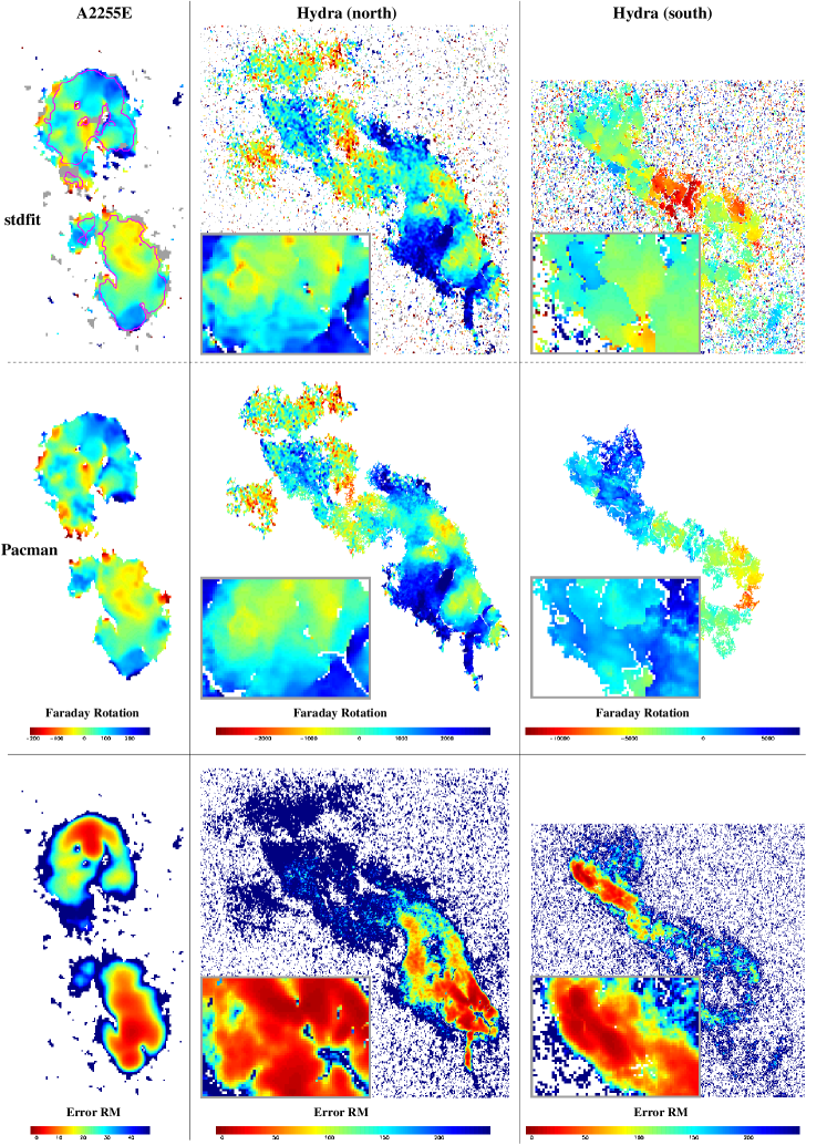
Figure 1: Comparison of the standard fit RM maps (upper panels) and the Pacman RM maps (middle panels) for A2255E (left column), the north (middle column) and the south lobe (right column) of Hydra A. RM values not represented by the colour bar are coloured in grey. Panels at the bottom exhibit the respective $\sigma^{{\rm RM}}$-maps. For the standard fit RM map of A2255E a $\sigma_{k}^{\max}=25\degr$ and $k_{min}=f=4$ was used, contours indicate the area covered by a standard fits RM map with $\sigma_{k}^{\max}=10\degr$. The parameters used for the Pacman RM map of A2255E are $\sigma_{k}^{\max}=25\degr$, $\sigma^{\Delta}_{\max}=25\degr$, $g$ = 1.2 and $k_{min}=f=4$; for the standard fit RM maps of Hydra A are $\sigma_{k}^{\max}=25\degr$ and $k_{min}=f=4$ (at 8 GHz); for the Pacman RM map of Hydra (north) are $\sigma_{k}^{\max}=30\degr$, $k_{min}=4$, $f=5$, $\sigma^{\Delta}_{\max}=25\degr$ and $g$ = 1.5; for the Pacman RM map of Hydra (south) are $\sigma_{k}^{\max}=35\degr$, $k_{min}=f=5$, $\sigma^{\Delta}_{\max}=35\degr$ and $g$ = 2.0.

3.1 Abell 2255E

The Abell cluster 2255, which has a redshift of 0.0806 (Struble & Rood, 1999), has been studied by Burns et al. (1995) and Feretti et al. (1997). The polarised radio source B1713+641, which we call hereafter A2255E, has a two sided radio lobe structure and is not directly located in the cluster centre. Polarisation observations were performed using the Very Large Array (VLA) at 4535, 4885, 8085, and 8465 MHz. The data reduction was done with standard AIPS (Astronomical Imaging Processing Software) routines (Govoni et al., in prep.). The polarisation angle maps and their standard error maps for the four frequencies were kindly provided to us by Federica Govoni. A preliminary analysis of an RM map of this source in order to determine the properties of the magnetic field in the intra-cluster gas in Abell 2255 is presented in Govoni et al. (2002).

Using the polarisation angle data, an RM map employing the standard fit algorithm was calculated, where the maximal allowed error in polarisation angle was chosen to be $\sigma_{k}^{\max}=25\degr$. The resulting RM map is shown in the upper left panel of Fig 1. The overlaid contour indicates the area which would be covered if polarisation angle errors were limited by $\sigma_{k}^{\max}=10\degr$. For these calculations, we assumed ${\rm RM}^{\max}=1\,500$ rad m^-2.

As can be seen from this map, typical RM values range between -100 rad m^-2 and +210 rad m^-2. Since this cluster is not known to inhabit a cooling core in its centre (Feretti et al., 1997), these are expected values. However, the occurrence of RM values around 1000 rad m^-2, which can be seen as grey areas in the standard fit map of A2255E, might indicate that for these areas the $n\pi$-ambiguity was not properly solved. One reason for this suspicion is found in the rapid change of RM values occurring between 1 or 2 pixel from 100 to 1000 rad m^-2. All these jumps have a $\Delta{\rm RM}$ of about 1000 rad m^-2 indicating $n\pi$-ambiguities between 4 GHz and 8 GHz which can be theoretically calculated from $\Delta{\rm RM}=\pi/(\lambda_{2}^{2}-\lambda_{1}^{2})$. Another important point to note is that parts of the grey areas lie well within the $\sigma_{k}^{\max}=10\degr$ contour, and hence, contribute to the results of any statistical analysis of such a parametrised RM map.

Therefore, the polarisation data of this source provide a good possibility to demonstrate the robustness and the reliability of our proposed algorithm. The RM map calculated by Pacman is shown in the middle left panel. The same numbers for the corresponding parameters were used; $\sigma_{k}^{\max}=25\degr$, ${\rm RM}^{\max}=1\,500$ rad m^-2.

An initial comparison by eye reveals that the method used in the standard fit procedure produces spurious RMs in noisy regions (manifested as grey areas in the upper left panel of Fig. 1) as previously mentioned while the RM map calculated by Pacman shows no such grey areas. The apparent jumps of about 1000 rad m^-2 observed in the standard fit map have disappeared in the Pacman map. Note, that in principle by realising that these steps are due to $n\pi$-ambiguities, one could re-run the standard fit algorithm with a lower ${\rm RM}_{\max}$ and this wrong solutions would disappear. However, by doing this a very strong bias is introduced since there might also be large RM values which are real. This bias can be easily relaxed by using Pacman.

A pixel-by-pixel comparison is shown in Fig. 2. In this figure the ${\rm RM}_{\rm{stdfit}}$ values obtained for pixels using a standard fit are plotted on the $y$-axis against the ${\rm RM}_{\rm{Pacman}}$ values obtained at the same corresponding pixel locations using the Pacman algorithm on the $x$-axis. The black points represent the error weighted standard fit whereas the red points represent the non-error weighted standard fit. Note that Pacman applied only an error weighted least-squares fit to the data. From this scatter plot, one can clearly see that both methods yield same RM values for most of the points which is expected from the visual comparison of both maps. However, the points for ${\rm RM}_{\rm{stdfit}}$ values at around $\pm$ 1000 rad m^-2 are due to the wrong solution of the $n\pi$-ambiguity found by the standard fit algorithm.

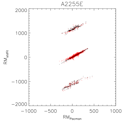
Figure 2: A pixel-by-pixel scatter plot of ${\rm RM}_{\rm{stdfit}}$ values obtained using the standard fit on the $y$-axis versus the ${\rm RM}_{\rm{Pacman}}$ values calculated from the polarisation data of Abell 2255 by employing our new algorithm Pacman. Black points represent results from an error weighted standard least-squares fit and red points from a non-error weighted standard fit. The points for ${\rm RM}_{\rm{stdfit}}$ values of around $\pm$ 1000 ${\mathrm{rad}}\,{\mathrm{m}}^{-2}$ are artefacts of a wrong solution of the $n\pi$-ambiguity.

For the demonstration of the effect of $n\pi$-ambiguity artefacts and pixel noise on statistical analysis, we determined the cluster magnetic field power spectra by employing the approach briefly described in Sect. 2.3. For detailed discussion and description of the application of the method to data, we refer the reader to Vogt & Enßlin (2003). In the calculation, we assumed that the source plane is parallel to the observer plane. Please note, that the application of an RM data filter in order to remove bad data or data which might suffer from a wrong solution to the $n\pi$-ambiguity as described by Vogt & Enßlin (2003) is here not necessary and not desirable. This is on the one hand due to the use of an error weighting scheme in the window function to suppress bad data and on the other hand due to the wish to study the influence of noise and map making artefacts on the power spectra.

The RM area used for the calculation of any power spectrum is the RM area which would be covered by the Pacman algorithm while using the same set of parameter $\sigma_{k}^{\max}$, ${\rm RM}^{max}$. This ensures that pixels on the border or noisy regions of the image not associated with the source – as seen in the standard fit RM map of A2255E in the upper left panel of Fig. 1 – are not considered for the analysis. (The same philosophy also applies for the discussion of the Hydra data in Sect. 3.2 and Sect. 3.3).

The power spectra calculated for various map making scenarios are shown in Fig. 3. The solid and dashed line represent power spectra calculated from standard fit RM maps. The solid line was calculated from an RM map which was obtained by using $\sigma_{k}^{\max}=20\degr$ where no error weighting was applied to the standard fit. The possible window weighting as introduced in Sect. 2.3 was also not applied. This scenario is therefore considered as a worst case. The dashed line was calculated from an RM map employing an error weighted standard fit while only allowing errors in the polarisation angle of $\sigma_{k}^{\max}=10\degr$. Again no window weighting was applied. From the comparison of these two power spectra alone, one can see that the large $k$-scales – and thus small real space scales – are sensitive to pixel-noise. Therefore, the application of an error weighted least square fit in the RM calculation leads to a reduction of noise in the power spectra. Note that in these two power spectra, the influence of the $n\pi$-artefacts are still present even in the error weighted standard fit RM map.

Figure 3: Various power spectra for the cluster Abell 2255 determined from different RM map making scenarios are shown. The solid line represents a power spectrum calculated from a standard fit RM map with $\sigma_{k}^{\max}=20\degr$ where no error weighting was applied. The dashed power spectrum was obtained from a standard fit RM map with $\sigma_{k}^{\max}=10\degr$ where error weighting was applied to the standard fit. The dashed-dotted power spectrum was determined from a Pacman RM map with $\sigma_{k}^{\max}=20\degr$ and error weighting was applied to the RM fits. The dotted line represents a power spectrum calculated from a Pacman RM map as above, but additionally a simple window weighting was applied for the determination of the power spectra. For comparison, the power spectra of pure white noise is plotted as a straight dashed line.

The two remaining power spectra in Fig. 3 allow us to investigate the influence of the $n\pi$-artefacts. The dashed-dotted line represents the power spectra as calculated from a Pacman RM map allowing $\sigma_{k}^{\max}=20\degr$ performing an error weighted fit. Again, no window weighting was applied to this calculation. One can clearly see that there is one order of magnitude difference between the error weighted standard fit power spectra and the Pacman one at large $k$-values. Since we also allow higher noise levels $\sigma_{k}^{\max}$ for the polarisation angles, this drop can only be explained by the removing of the $n\pi$-artefacts in the Pacman map. That there is still a lot of noise in the map on small real space scales (large $k$’s), which governs the power spectra on these scales, can be seen from the dotted power spectrum, which was determined as above while applying a simple window weighting in the calculation. There is an additional difference of about one order of magnitude between the two power spectra at large $k$-scales determined for the two Pacman scenarios.

For comparison the power spectrum of pure white noise is plotted as straight dashed line in Fig. 3. It can be shown analytically, that white noise as observed through an arbitrary window results in a spectrum of $\varepsilon_{B}(k)\propto k^{2}$.

As another independent statistical test, we applied the gradient vector alignment statistic $\tilde{V}$ to the RM and $\varphi^{0}$ maps calculated by the Pacman and the standard fit algorithm. The gradients of RM and $\varphi^{0}$ were calculated using the scheme as described in footnote 5 in Enßlin et al. (2003). For the two RM maps shown in Fig. 1, we find a ratio of $\tilde{V}_{\rm{stdfit}}/\tilde{V}_{\rm{pacman}}=20$, which indicates a significant improvement mostly resulting from removing the $n\pi$-artefacts by the Pacman algorithm. The calculation of the normalised quantity $V$ yielded $V_{\rm{stdfit}}=-0.75$ and $V_{\rm{pacman}}=-0.87$. Smoothing the Pacman RM map slightly leads to a drastic decrease of the quantities $\tilde{V}$ and $V$. This indicates that the statistic is still governed by small scale noise. This can be understood by looking at the RM maps of Abell 2255 in Fig. 1. The extreme RM values are situated at the margin of the source which is, however, also the noisiest region of the source. Calculating the normalised quantity for the high signal-to-noise region yields $V_{\rm{pacman}}=-0.56$. For comparison, the normalised quantity for the standard fit of the same high signal-to-noise region is $V_{\rm{stdfit}}=-0.94$.

3.2 Hydra North

The polarised radio source Hydra A, which is in the centre of the Abell cluster 780, also known as the Hydra A cluster, is located at a redshift of 0.0538 (de Vaucouleurs et al., 1991). The source Hydra A shows an extended, two-sided radio lobe. Detailed X-ray studies have been performed on this cluster (e.g. Ikebe et al., 1997; Peres et al., 1998; David et al., 2001). They revealed a strong cooling core in the cluster centre. The Faraday rotation structure was observed and analysed by Taylor & Perley (1993). They reported RM values ranging between $-1\,000$ rad m^-2 and $+3\,300$ rad m^-2 in the north lobe and values down to $-12\,000$ rad m^-2 in the south lobe.

Polarisation angle maps and their error maps for frequencies at $7\,815$, $8\,051$, $8\,165$, $8\,885$ and $14\,915$ MHz resulting from observation with the Very Large Array were kindly provided to us by Greg Taylor. A detailed description of the radio data reduction can be found in Taylor et al. (1990) and Taylor & Perley (1993).

Figure 4: A pixel-by-pixel comparison for the Hydra north lobe of $RM_{\rm{stdfit}}$ values obtained using the standard fit plotted on the $y$-axis versus the ${\rm RM}_{\rm{Pacman}}$ values calculated by employing our new algorithm Pacman. The parallel scattered points at $\pm$ 3000-4000 rad m^-2 and $\pm\,10\,000$ rad m^-2 are a result of spurious solutions to the $n\pi$-ambiguity obtained by the standard fit algorithm. For the calculation of the RM maps, all five frequencies were used.

In this section, we concentrate on the north lobe of Hydra A and discuss the south lobe separately in Sect. 3.3. The south lobe is more depolarised, leading to a lower signal-to-noise than in the north lobe. The north lobe is a good example of how to treat noise in the data, while the south lobe gives a good opportunity to discuss the limitations and the strength of our algorithm Pacman.

Using the polarisation data for the four frequencies at around 8 GHz, we calculated the standard fit RM map which is shown in the upper middle panel of Fig. 1. The maximal allowed error in polarisation angle was chosen to be $\sigma_{k}^{\max}=25\degr$ and RM${}^{\max}=15\,000$ rad m^-2. A Pacman RM map is shown in the middle of the middle panel in Fig. 1 below the standard fit map. This map was calculated using the four frequencies at around 8 GHz with a $\sigma_{k=8GHz}^{\max}=30\degr$ and additionally where possible the fifth frequency at 15 GHz was used with a $\sigma_{k=15GHz}^{\max}=35\degr$. RM^max was chosen to be $15\,000$ rad m^-2. From a visual comparison of the two maps, one can conclude that the standard fit map looks more structured on smaller scales and less smooth than the Pacman map. This structure on small scales might be misinterpreted as small scale structure of the RM producing magnetic field. Note that the difference in the RM maps is mainly due to the usage of the fifth frequency for the Pacman map demonstrating that all information available should be used for the calculation of RM maps in order to avoid misinterpretation of the data.

Since the four frequencies around 8 GHz are close together, a wrong solution of the $n\pi$-ambiguity would manifest itself by differences of about $\Delta{\rm RM}=10\,000$ rad m ^-2. Such jumps are not observed in the main patches of the standard fit RM map shown in Fig. 1. However, including the information contained in the polarisation angle map of the 5th frequency at 15 GHz, which is desirable as explained above, one introduces the possibility of $n\pi$-ambiguities resulting in $\Delta{\rm RM}=3\,000...4\,000$ rad m^-2. Therefore, a scatter plot of a pixel-by-pixel comparison between a standard fit and a Pacman map, calculated both using the additional available information on the fifth frequency, is shown in Fig. 4. The parallel scattered points are spurious solutions found by the standard fit algorithm. One can clearly see that they develop at $\pm$ 3000-4000 rad m^-2 and less pronounced at $\pm\,10\,000$ rad m^-2.

As we will discuss below, the 15 GHz data set may have a lower signal–to–noise ratio than the 8 GHz data and thus, a lower error threshold $\sigma_{k}^{\max}$ will eliminate most of the wrong fits. However, it is a particular strength of Pacman that it yields still reliable results even if choosing larger error thresholds.

Figure 5: Various power spectra calculated for the RM maps for the north lobe of Hydra A are shown. The dashed dotted line and the dotted line represent the power spectra calculated from the standard fit RM map and the Pacman RM map, respectively, while no window weighting was applied. A threshold window weighting assuming a $\sigma_{0}^{{\rm RM}}$ = 75 rad m^-2 yield the dashed line power spectrum for the standard fit map and the solid line for the Pacman map. The standard fit maps were calculated from the four frequencies at 8 GHz whereas the Pacman maps were determined using additionally the fifth frequency when possible. For both algorithms, $\sigma_{k}^{\max}=35\degr$ was used. The influence of the small–scale pixel noise on the power spectra can clearly be seen in this figure at large $k$-values.

In order to study the influence of the noise on small scales, we calculated the power spectra from RM maps obtained using different parameter sets for the Pacman and the standard fit algorithm. As for Abell 2255E, all calculations of power spectra were done for RM areas which would be covered by the Pacman fit if the same parameters were used. Again this leads to exclusion of pixels in the standard fit RM map which are not associated with the source.

There is a clear depolarisation asymmetry of the two lobes of Hydra A observed as described by the Laing–Garrington effect (Taylor & Perley, 1993; Lane et al., 2004). Therefore, we assume for the calculation of any power spectra for the Hydra source, that the source plane is tilted by an inclination angle of 45$\degr$ where the north lobe points towards the observer and the south lobe away from the observer.

For a first comparison, we calculated the power spectra for two RM maps similar to the one shown in Fig. 1. They were obtained using the four frequencies at 8 GHz for the standard fit algorithm and using additionally the fifth frequency when possible for the Pacman algorithm. The other parameters were chosen to be $\sigma_{k}^{\max}=35\degr$ and ${\rm RM}^{\max}=15\,000$ rad m^-2. For these two RM maps, we determined power spectra applying firstly no window weighting at all and secondly threshold window weighting as described in the end of Sec. 2.3. We choose the threshold to be $\sigma_{0}^{{\rm RM}}$ = 75 rad m^-2 which represents the high signal-to-noise region. The respective spectra are exhibited in Fig. 5.

For the power spectra, $n\pi$-artefacts should play only a minor role in the calculation of the power spectra as explained above. Therefore, any differences arising in these spectra are caused by the varying treatment of noise in the map making process or in the analysis. Comparing the power spectra without window weighting, the one obtained from the Pacman RM map lies below the one from the standard fit RM map. The difference is of the order of half a magnitude for large $k$’s – small real space scales. The standard fit power spectrum seems to increase with larger $k$ but the Pacman one seems to decrease over a greater range in $k$. The reason for this difference is the same one which was responsible for the different smoothness in the two RM maps shown in Fig. 1, namely that only four frequencies were used for the standard fit RM map. Even introducing a window weighting scheme, which down-weights noisy region, cannot account entirely for that difference as can be seen from the comparison of the window weighted power spectra. This is especially true because the small-scale spatial structures are found even in the high signal-to-noise regions when using only four frequencies for the RM map calculation. This demonstrates again how important it is to include all available information in the map making process.

In order to study the influence of the maximal allowed measurement error in the polarisation angle $\sigma_{k}^{\max}$, we calculated the power spectra for a series of Pacman RM maps obtained for $\sigma_{k}^{\max}$ ranging from 5$\degr$ to 35$\degr$. The RM maps were derived using all five frequencies $k_{\min}$= 5, not allowing any points to be considered for which only four frequencies fulfil $\sigma_{k_{ij}}<\sigma_{k}^{\max}$. Again an $RM^{\max}=15\,000$ rad m^-2 was used. The resulting power spectra using a threshold window weighting ($\sigma_{0}^{{\rm RM}}$ = 50 rad m^-2) are exhibited in Fig. 6. One can see that they are stable and do not differ substantially from each other even though the noise level increases slightly when increasing the $\sigma_{k}^{\max}$. This demonstrates the robustness of our Pacman algorithm.

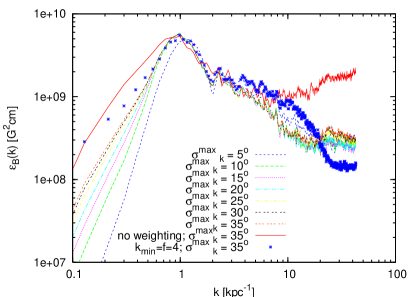
Figure 6: Power spectra for the north lobe of Hydra A calculated from a series of Pacman RM maps are shown. The various coloured dashed and dotted lines show power spectra from RM maps calculated for $\sigma_{k}^{\max}$ ranging from 5$\degr$ to 35$\degr$ using all five frequencies $k_{\min}=5$. The spectra were determined applying threshold window weighting ($\sigma_{0}^{{\rm RM}}$ = 50 rad m^-2). For comparison the solid red line power spectrum, which is the largest spectrum at $k>10$ kpc^-1, is not window weighted for $\sigma_{k}^{\max}=35\degr$. The power spectrum represented by the blue stars was derived from an Pacman RM map obtained using the four frequencies at 8 GHz and a $\sigma_{k}^{\max}=35\degr$.

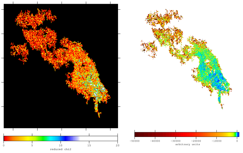
Figure 7: On the left hand side a $\chi^{2}_{\nu{ij}}$ is shown. The yellow and green regions have values larger than unity indicating underestimation of errors. Note that for these regions the RM fit used five frequencies whereas in the outer parts of the source only four frequencies were used. A $\tilde{V}$ map for the north lobe of Hydra A is exhibited on the right panel. The extreme negative values (red and black) correspond to strong anti-correlation of RM and $\varphi^{0}$ fluctuations, which are produced by noise in the observed maps. However, the green and blue coloured regions have values around zero and are therefore high signal-to-noise regions (compare with the $\sigma^{{\rm RM}}$ map in the middle panel of Fig. 1).

For comparison, we plotted two more power spectra in Fig. 6. For the solid red line spectrum, no window weighting was applied to an RM map which was calculated as above having $\sigma_{k}^{\max}=35\degr$. One can clearly see that the spectrum is governed by noise on large $k$-scales – small real space scales. Thus, some form of window weighting in the calculation of the power spectra seems to be necessary in order to suppress a large amount of noise.

Another aspect arises in the noise treatment if we consider the power spectra represented by the blue stars which was calculated using a threshold window weighting ($\sigma_{0}=$ 50 rad m^-2). This power spectrum represents the analysis for an RM map obtained using only the four frequencies at 8 GHz while $\sigma_{k}^{\max}=35\degr$. It is striking that the noise level on large $k$-scales (on small real space scales) is lower than for the RM maps obtained for the five frequencies, one would expect it to be the other way round. Apparently the fifth frequency has a lot of weight in the determination of $\sigma^{{\rm RM}}_{ij}$ (see Eq. (3) in paper I) since this frequency is almost twice as large as the other four. If the measurement errors of the polarisation angles are underestimated this can lead to an underestimation of the uncertainty $\sigma^{{\rm RM}}_{ij}$ in the final RM value due to Gaussian error propagation. A more accurate error estimate could be achieved by considering the error treatment as described by Johnson et al. (1995). They state in their Appendix that errors are not uniform across synthesis images and propose a different error algorithm.

One can test the hypothesis of underestimation of errors by performing a $\chi^{2}_{\nu}$ test as described in Sect. 2.2. The $\chi^{2}_{\nu_{ij}}$ map for the Pacman RM map of Hydra North derived by using a multi-frequency fit (see middle upper panel of Fig. 1) is exhibited in the left panel of Fig. 7. The red values are close to unity. However the yellow and blue regions in this map are values larger than unity indicating that the errors are underestimated in these regions. Note that in these regions there is also the fifth frequency used for the RM fit which might indicate that the errors for this frequency are underestimated by a larger factor than for the other four frequencies.

We also applied the gradient vector product statistic $\tilde{V}$ to the RM and $\varphi^{0}$ maps obtained by using the RM maps as shown in the middle panel of Fig. 1 and the respective $\varphi^{0}$ maps. The calculation yielded for the ratio $\tilde{V}_{\rm stdfit}/\tilde{V}_{\rm pacman}=1.2$. This corresponds to a slight decrease of correlated noise in the Pacman maps. The calculation of the normalised quantity resulted in $V_{\rm stdfit}=-0.85$ for the standard fit and $V_{\rm pacman}=-0.83$ for the Pacman maps. This is expected since the low signal-to-noise areas of the north lobe of Hydra A will govern this gradient statistic and for both RM maps these areas look very similar. In order to visualise this, we calculated a $\tilde{V}$ map which is exhibited in Fig. 7. The extreme negative values observed for the low signal-to-noise regions (red regions) indicate strong anti-correlation and thus, anti-correlated fluctuations of RM and $\varphi^{0}$ in these regions. For the high signal-to-noise regions (blue and green) moderate values varying around zero are observed. Note the striking morphological similarity of the RM error ($\sigma^{{\rm RM}}$) map in the lower middle panel of Fig. 1 and of the $\tilde{V}$ map as shown in Fig. 7. These two independent approaches to measure the RM maps accuracy give a basically identical picture. These approaches are complementary since they use independent information. The RM error map is calculated solely from $\sigma_{k}$ maps, which are based on the absolute polarisation errors, whereas the $\tilde{V}$ map is based solely on the RM derived from the polarisation angle $\varphi(k)$ maps.

However, we note that the results for magnetic field strengths and correlation lengths presented by Vogt & Enßlin (2003) are not changed substantially. This is owing to the fact that Vogt & Enßlin (2003) considered for the calculation of the magnetic field properties only the power on scales which were larger than the resolution element (beam). Therefore the small scale noise was not considered for this calculation and thus, no change in the results given is expected. The central magnetic field strength for this cluster as derived during the course of this work is about 10 $\mu$G and the field correlation length is about 1 kpc being consistent with results presented in Vogt & Enßlin (2003).

3.3 The Quest for Hydra South

As already mentioned, the southern part of the Hydra source has to be addressed separately, as it differs from the northern part in many respects. One of them is that the depolarisation is higher in the south lobe which especially complicates the analysis of this part.

An RM map obtained employing the standard fit algorithm using the four frequencies at 8 GHz is shown in the upper right panel of Fig. 1. This RM map exhibits many jumps in the RM distribution which seems to be split in lots of small patches having similar RMs. Furthermore, RMs of $-12\,000$ rad m^-2 are detected (indicated as red regions in the map). If one includes the fifth frequency at 15 GHz in the standard fit algorithm, the appearance of the RM map does not change significantly, and most importantly, the extreme values of about $-12\,000$ rad m^-2 do not vanish.

The application of the Pacman algorithm with conservative settings for the parameters $\sigma_{k}^{\max}$, $\sigma^{\Delta}_{\max}$ and $g$, leads to a splitting of the RM distribution into many small, spatially disconnected patches. Such a map does look like a standard fit RM map and there are still the RM jumps and the extreme RM values present. However, if one lowers the restrictions for the construction of patches, the Pacman algorithm starts to connect patches to the patch with the best quality data available in the south lobe using its information on the global solution of the $n\pi$-ambiguity. An RM map obtained pushing Pacman to such limits is exhibited in the middle right panel of Fig. 1. Note that the best quality area is covered by the bright blue regions and a zoom-in for this region is also exhibited in the small box to the lower left of the source. In the lowest right panel of Fig. 1, a $\sigma^{RM}$-map is shown indicating the high quality regions by the red colour.

Figure 8: An example for individual RM fits across an RM jump observed in the RM maps of the south lobe of Hydra A. The solid line indicates the standard fit solution and the dashed one represents the Pacman solution. The error bars in these plots indicate the polarisation errors which were multiplied by 3. Note that this is an extreme example, where Pacman chooses a solution to the individual fits in noisy regions which has not necessarily the minimal $\chi^{2}$ value by construction. However, the global statistical tests applied to the whole RM map of Hydra South indicate that the Pacman map has less artefacts in comparison to the standard fit RM map. We note, that for this particular local example it is not trivial to decide which algorithm is giving the right solution.

The RM distribution in this Pacman map exhibits clearly fewer jumps than the standard fit map although the jumps do not vanish entirely. Another feature that almost vanishes in the Pacman map are the extreme RMs of about $-12\,000$ rad m^-2. The RM distribution of the Pacman map seems to be smoother than the one of the standard fit map. However, if the individual RM fits for points, which deviate in their RM values depending on the algorithm used, are compared in a $\varphi(k)$-$\lambda_{k}^{2}$-diagram, the standard fit seems to be the one which would have to be preferred since it does fit better to the data at hand. Pacman has some resistance to pick this smallest $\chi^{2}$ solution if it does not make sense in the context of neighbouring pixel information. As an example, we plotted individual RM fits which are observed across the RM jumps in Fig. 8. However as shown above, one has to consider that the measurement errors might be underestimated which gives much tighter constraints on the fit than it would otherwise be.

Figure 9: Various power spectra for the RM maps of the south lobe of the Hydra source are compared with the power spectrum of the north lobe calculated from the Pacman RM map ($k_{\min}=5$, $\sigma_{k}^{\max}=35\degr$) employing a threshold weighting with $\sigma_{0}^{{\rm RM}}=50$ rad m^-2 represented as filled circles.

In order to investigate these maps further, we also calculated the threshold weighted ($\sigma_{0}^{{\rm RM}}$ = 50 rad m^-2) and simple weighted power spectra from the Pacman and the standard fit RM maps of the south lobe and compared them to the one from the north lobe. The RM maps used for the comparison were all calculated employing $\sigma_{k}^{\max}=35\degr$ and $k_{\min}=f=5$. The various power spectra are shown in Fig. 9. One can clearly see that the power spectra calculated for the south lobe lie well above the power spectra from the north lobe, which is represented as filled circles.

Concentrating on the comparison of the simple window weighted power spectra of the south lobe in Fig. 9 (solid line from Pacman RM map and dashed line from standard fit RM map) to the one of the north lobe, one finds that the power spectrum calculated from the Pacman RM map is closer to the one from the north lobe than the power spectrum derived from the standard fit RM map. This indicates that Pacman RM map might be the right solution to the RM determination problem for this part of the source. However, this difference vanishes if a different window weighting scheme is applied to the calculation of the power spectrum. This can be seen by comparing the threshold window weighted power spectra (dotted line for the power spectra of the Pacman RM map and dashed dotted line for the power spectra from the standard fit RM map) in Fig. 9. Since the choice of the window weighting scheme seems to have also an influence on the result the situation is still inconclusive.

An indication for the right solution of the $n\pi$-ambiguity problem may be found in the application of our gradient vector product statistic $\tilde{V}$ to the Pacman maps and the standard fit maps of the south lobe (as shown in Fig. 1). The calculations yielded a ratio $\tilde{V}_{\rm{stdfit}}/\tilde{V}_{\rm{pacman}}=12$. This is a difference of one order of magnitude and represents a substantial decrease in correlated noise in the Pacman maps. The calculation of the normalised quantity yielded $V_{\rm{stdfit}}=-0.69$ for the standard fit maps and $V_{\rm{pacman}}=-0.47$ for the Pacman maps. This result strongly indicates that the Pacman map should be the preferred one.

The final answer to the question about the right solution of the RM distribution problem for the south lobe of Hydra A has to be postponed until observations of even higher sensitivity, higher spatial resolutions and preferably also at different frequencies are available.

4 Conclusions & Lessons

We demonstrated the robustness of our Pacman algorithm which is especially useful for the calculation of RM and $\varphi^{0}$ maps of extended radio sources. It dramatically reduces $n\pi$-artefacts in noisy regions and makes the unambiguous determination of RMs in these regions possible. Any statistical analysis of the RM maps will profit from this improvement.

In the course of this work the observational data taught us the following lessons:

1. It is important to use all available information obtained by the observation. It seems especially desirable to have a good frequency coverage. The result is a smoother, less noisy map.

2. For the individual least-squares fits of the RM, it is advisable to use an error weighting scheme in order to reduce the noise.

3. Global algorithms are preferable, if reliable RM values are needed from low signal-to-noise regions at the edge of the source.

4. Sometimes it is necessary to test many values of the parameters ${\rm RM}^{\max}$, $\sigma^{\max}_{k}$ and $\sigma^{\Delta}_{\max}$, which govern the Pacman algorithm, in order to investigate the influence on the resulting RM maps.

5. One has to keep in mind that whichever RM map seems to be most believable, it might still contain artefacts. One should do a careful analysis by looking on individual RM pixel fits but one also should consider the global RM distribution. We presented the gradient vector product statistic $\tilde{V}$ as a useful tool to estimate the level of reduction of cross-correlated noise in the calculated RM and $\varphi^{0}$ maps.

6. For the calculation of power spectra it is always preferable to use a window weighting scheme which has to be carefully selected.

7. Finally, under or overestimation of the measurement errors of polarisation angles (which will propagate through all calculations due to error propagation) could influence the final results. We performed a reduced $\chi^{2}_{\nu}$ test in order to test if the errors are over or under estimated.

We conclude that the calculation of RM maps is a very difficult task requiring a critical view to the data and a careful noise analysis. However, we are confident that Pacman offers a good opportunity to calculate reliable RM maps and to understand the data and its limitations better. Furthermore, such improved RM maps and the according error analysis for Hydra North and Abell 2255 were presented in this paper.

References

- Burns et al. (1995) Burns J. O., Roettiger K., Pinkney J., Perley R. A., Owen F. N., Voges W., 1995, ApJ, 446, 583
- David et al. (2001) David L. P., Nulsen P. E. J., McNamara B. R., Forman W., Jones C., Ponman T., Robertson B., Wise M., 2001, ApJ, 557, 546
- de Vaucouleurs et al. (1991) de Vaucouleurs G., de Vaucouleurs A., Corwin H. G., Buta R. J., Paturel G., Fouque P., 1991, Third Reference Catalogue of Bright Galaxies. Volume 1-3, XII, Springer-Verlag Berlin Heidelberg New York
- Dolag et al. (2003) Dolag K., Vogt C., Enßlin T. A., 2003, MNRAS, submitted
- Enßlin & Vogt (2003) Enßlin T. A., Vogt C., 2003, A&A, 401, 835
- Enßlin et al. (2003) Enßlin T. A., Vogt C., Clarke T. E., Taylor G. B., 2003, ApJ, 597, 870
- Feretti et al. (1997) Feretti L., Boehringer H., Giovannini G., Neumann D., 1997, A&A, 317, 432
- Govoni et al. (2002) Govoni F., Feretti L., Murgia M., Taylor G. B., Giovannini G., Dallacasa D., 2002, in ASP Conf. Series: Matter and Energy in Clusters of Galaxies Magnetic Fields in Clusters of Galaxies Obtained Through the Study of Faraday Rotation Measures. pp arXiv:astro–ph/0211292
- Haves (1975) Haves P., 1975, MNRAS, 173, 553
- Ikebe et al. (1997) Ikebe Y., Makishima K., Ezawa H., Fukazawa Y., Hirayama M., Honda H., Ishisaki Y., Kikuchi K., Kubo H., Murakami T., Ohashi T., Takahashi T., Yamashita K., 1997, ApJ, 481, 660
- Johnson et al. (1995) Johnson R. A., Leahy J. P., Garrington S. T., 1995, MNRAS, 273, 877
- Lane et al. (2004) Lane W. M., Clarke T. E., Taylor G. B., Perley R. A., Kassim N. E., 2004, AJ, 127, 48
- Peres et al. (1998) Peres C. B., Fabian A. C., Edge A. C., Allen S. W., Johnstone R. M., White D. A., 1998, MNRAS, 298, 416
- Ruzmaikin & Sokoloff (1979) Ruzmaikin A. A., Sokoloff D. D., 1979, A&A, 78, 1
- Sarala & Jain (2001) Sarala S., Jain P., 2001, MNRAS, 328, 623
- Struble & Rood (1999) Struble M. F., Rood H. J., 1999, ApJS, 125, 35
- Taylor & Perley (1993) Taylor G. B., Perley R. A., 1993, ApJ, 416, 554
- Taylor et al. (1990) Taylor G. B., Perley R. A., Inoue M., Kato T., Tabara H., Aizu K., 1990, ApJ, 360, 41
- Vallée & Kronberg (1975) Vallée J. P., Kronberg P. P., 1975, A&A, 43, 233
- Vogt & Enßlin (2003) Vogt C., Enßlin T. A., 2003, A&A, 412, 373