DIAGNOSTICS OF NEUTRON STAR AND BLACK HOLE X-RAY BINARIES WITH X-RAY SHOT WIDTHS

Abstract

A statistic $w$, the differential coefficient of the mean absolute difference of an observed lightcurve, is proposed for timescale analysis of shot widths. The shortest width of random shots can be measured by the position of the lower cut-off in the timescale spectrum of $w$. We use the statistic to analyze X-ray lightcurves from a sample of neutron star and black hole binaries and the results show that the timescale analysis can help us distinguish between neutron star binaries and black hole binaries. The analysis can further reveal the structure and dynamics of accretion disks around black holes.

1 Introduction

Complex X-ray emission variability at wide timescales has been observed in accreting stellar mass black hole candidate (BHC) and weakly magnetized neutron stars (NS) systems (for reviews see Tanaka & Lewin, 1995; van der Klis, 1995). On the subsecond timescale, aperiodic fluctuations are common in these systems, as first discovered by Oda et al. (1971) in the prototype BHC Cyg X-1 in its hard state with a large amplitude (up to $\sim 40\%$ rms of the mean flux). Many properties of X-ray rapid variability from Cyg X-1, e.g., the Fourier power spectrum, the mean and variance, and the autocorrelation function of the lightcurve, could be described as the superposition of individual shots with the characteristic duration of a few tenths of a second (Terrel, 1972; Oda, 1977; Sutherland, Weisskopf & Kahn, 1978; Nolan et al., 1981; Meekings et al., 1984; Miyamoto et al., 1988, 1992; Lochner, Swank, & Szymkowiak, 1991). The average shot profiles of Cyg X-1 have been obtained by superposing many shots by aligning their peaks in the lightcurves obtained with Ginga (Negoro, Miyamoto, & Kitamoto, 1994; Negoro, Kitamoto, & Mineshige, 2001) and RXTE (Feng, Li, & Chen, 1999).

Studying the short timescale variability of the X-ray emission of accreting BHC or NS systems is important for understanding the emitting region and emission process of high energy photons, as well as the nature of the compact object. Timing studies carried out in the time domain can make direct measurements of, e.g., power, spectral lag, of a stochastic process at high frequencies (short timescales). Li (2001) has developed a technique of timescale analysis, with which timescale spectra can be derived directly in the time domain. The timescale analysis of the correlation coefficient between intensity and hardness ratio of Cyg X-1 (Li, Feng, & Chen, 1999) is consistent with the results from superposed shots (Feng, Li, & Chen, 1999; Negoro, Kitamoto, & Mineshige, 2001). The time domain power density at a certain timescale can be defined as the differential of the variation power in a lightcurve with the corresponding time step (Li, 2001). The timescale spectra of power density of a sample of NS and BHC binaries were analyzed and the results indicate that the characteristic timescale of hard X-ray shots is $\sim 0.1$ s for BHCs, and much shorter ($\ll 1$ ms) for NSs (Li & Muraki, 2002).

In the present work, we propose a statistic $w$, the differential coefficient of the mean absolute difference of an observed lightcurve, to make timescale analysis of shot width. The timescale spectrum of $w$ can reflect the width distribution of a stochastic shot process with noise. We introduce the method of $w$ analysis in §2. We studied the $w$ spectra of a sample of NS and BHC binaries and made an energy dependent analysis of the shot widths for three BHC binaries with RXTE/PCA data; the results are presented in §3. In §4 we discuss the possible implications of our results.

2 Method

2.1 Algorithm

Let $\{x(j;\delta t)\}$ denote the originally observed lightcurve, where $x(j;\delta t)$ (cts/s) is the counting rate during the time interval $[j\delta t,(j+1)\delta t)$ ($j=0,1,2,\ldots$), and $\delta t$ is the time resolution. To study the variability on a larger timescale $\Delta t=M\delta t$, we need to construct a lightcurve with the time step $\Delta t$ from the original time series by combining its M successive bins as

$$x_{m}(i;\Delta t)=\frac{1}{M}\sum_{j=iM+m}^{(i+1)M+m-1}x(j;\delta t)\quad\mbox{cts/s},$$ (1)

where $i=0,1,\ldots,N-1$ and $m$ ($\in[0,M-1]$) is the discrete phase of the time series. As the lightcurve $\{x_{m}(i;\Delta t)\}$ does not include any information about the variation on timescales shorter than $\Delta t$, it can be used to study the variability over the region of timescales $\geq\Delta t$. A mean absolute difference of the observed lightcurve at the timescale $\Delta t$ can be defined as

$$W(\Delta t)=\frac{1}{M}\sum_{m=0}^{M-1}(\frac{1}{N-1}\sum_{i=0}^{N-2}\frac{|x_{m}(i+1;\Delta t)-x_{m}(i;\Delta t)|}{\Delta t})~{}.$$ (2)

The quantity $W(\Delta t)$ includes information of variability with timescales larger than or equal to $\Delta t$. To extract the information at the timescale $\Delta t$, we can calculate the rate of change of $W(\Delta t)$

$$w(\Delta t)=-\frac{dW(\Delta t)}{d\Delta t}~{}.$$ (3)

To detect the signal in a spectrum $w(\Delta t)$ against a noise background, we need to know the timescale spectrum $w_{noise}(\Delta t)$ of a time series consisting of only noise. We assume two independent random variables $X_{1}$ and $X_{2}$ follow the Poisson distribution with the same mean $\overline{X}$ (cts), then the expectation of their absolute difference value is given by

$$E(|X_{1}-X_{2}|)=2e^{-2\overline{X}}\sum_{n=0}^{\infty}nI_{n}(2\overline{X})~{},$$ (4)

where $I_{n}$ is the modified Bessel function of the first kind with the order number $n$. Therefore the mean absolute difference for the background can be derived as

$$W_{noise}(\Delta t)=\frac{E(|X_{1}-X_{2}|)/\Delta t}{\Delta t}=\frac{2e^{-2\bar{x}\Delta t}\sum_{n=0}^{\infty}nI_{n}(2\bar{x}\Delta t)}{\Delta t^{2}}$$ (5)

with $\bar{x}$ being the average counting rate of the lightcurve, then

$$w_{noise}(\Delta t)=-\frac{dW_{noise}(\Delta t)}{d\Delta t}~{}.$$ (6)

Finally the signal’s value of the statistic $w$ can be derived as

$$w_{s}(\Delta t)=w(\Delta t)-w_{noise}(\Delta t)$$ (7)

Calculating $w_{s}(\Delta t)$ by Eq. (7) at different step $\Delta t$ for an observed lightcurve we can get a timescale spectrum of $w_{s}$. The differential coefficients in Eqs. (3) and (6) can be calculated numerically. In practice, a lightcurve may be divided into $L$ segments, we can calculate $w_{s,l}$ for each segment and then obtain the average value

$$\overline{w}_{s}=\sum_{l=0}^{L-1}w_{s,l}/L$$ (8)

and its standard error

$$\sigma(\overline{w}_{s})=\sqrt{\sum_{l=0}^{L-1}(w_{s,l}-\overline{w}_{{}_{s}})^{2}/L(L-1)}~{}.$$ (9)

2.2 Simulation

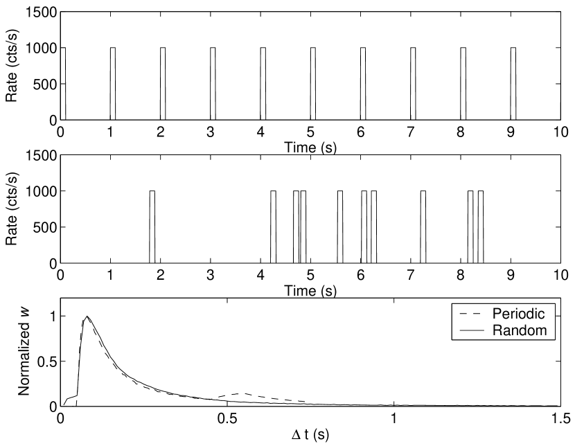
Figure 1: Timescale spectra of $w$ for periodic and random square signals. Top: a periodic square signal. The square width $t_{w}=0.1$ s and the period $T=1$ s. Middle: a random square signal. The square width $t_{w}=0.1$ s and the interval time between every two neighboring squares follows the exponential distribution with a mean of 1 s. Bottom: dashed line - the $w$ spectrum of the periodic signal; solid line - the $w$ spectrum of the random signal. The $w$ spectra reveal the main timescale $t_{w}$ of both series; the periodic process dominated by $T$ in the periodic series is revealed in the $w$ spectrum at $T/2$; larger amplitude at short timescales of the random series’s $w$ spectrum indicates the stronger variability at short timescales of the random series than the periodic one.

We make simulation study in order to understand the timescale spectra of $w$. The $w$ spectra of two time series consisting of square shots are calculated. The shot width is 0.1 s. One time series (top panel of 1) consists of periodic shots with a period of 1 s, and in the other time series (middle panel of 1) shots are randomly distributed with shot separations following an exponential distribution with a mean of 1 s. The time resolution is 5 ms and the total time length is 1250s with each segment of 250 s. A peak around the timescale 0.1 s appears clearly in each spectrum (see the bottom panel of Fig. 1). The other characteristic timescale of the periodic series, 0.5 s, is also shown in its $w$ spectrum (the dashed line in Fig. 1) with a smaller amplitude. At small timescales, the random shot series has stronger variability than the periodic one, indicated by the larger amplitude in the $w$ spectrum.

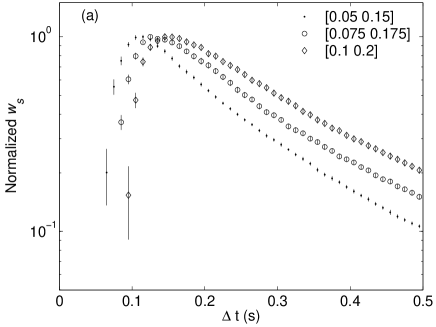
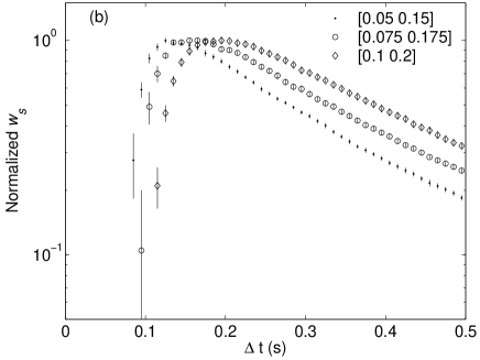
Figure 2: Timescale spectra of $w_{s}$ for randomly occurring shots. Shots separations are exponentially distributed with a mean of 1 s. The peak rate of a shot is random from 0 to 1000 cts/s above a background of 1000 cts/s. Poisson counting statistics are included in the simulations. The legend means the timescale regions in which shot width are randomly distributed (width refers to FWHM for Gaussian shots). (a) — $w$ spectra for square shots. (b) — $w$ spectra for Gaussian shots. (c) — PSDs for square shots. (d) — PSDs for Gaussian shots. The lower cut-off in each $w$ spectrum reflects the smallest shot width of the shot series. By fitting the cut-off edge of the $w$ spectrum, the shortest shot width can be measured (see details in §2.2). From the simulation, we can see $w$ spectrum is better than Fourier technique in shot width detection.

The $w_{s}$ spectra of a set of simulated lightcurves consisting of both white noise and signal shots randomly occurring with different widths and amplitudes are also calculated. The shot width is randomly sampled from a uniform distribution between $[\tau_{1},\tau_{2}]$ and its profile has either square or Gaussian form. The peak amplitude of a shot is drawn from a uniform distribution between 0 and 1000 cts/s. The shot occurring time is randomly distributed following an exponential distribution with a mean of 1 s. The time resolution is 10 ms and the total duration is 5000 s with each segment of 500 s. A background of 1000 cts/s is added. Poisson counting statistics are also included in the simulations. The results, shown in Fig. 2 (panel (a) for square shots and (b) for Gaussian shots), indicate that we can use the position of short timescale cut-off in the $w_{s}$ spectrum to measure the shortest width of random shots in an observed lightcurve with noise. For comparison, we also calculate the Fourier power spectrum density (PSD) for each shot series. The results are plotted in panel (c) and (d) of Fig. 2 for square and Gaussian shots, respectively. It is clear by comparing the PSD with the $w_{s}$ spectra in Fig. 2 that the $w$ spectrum can be used to detect the shot width more conveniently and accurately.

To measure the lower cut-off in a $w_{s}$ spectrum, we fit a polynomial to the front edge and obtain the root value. The error of the cut-off timescale is evaluated from the fitting error with 90% confident level. In this way, the lower cut-off timescales for the above simulations are $0.0614\pm 0.0006$, $0.0743\pm 0.0008$ and $0.0893\pm 0.0009$ (s) respectively for different lightcurves in the left panel of fig. 2, and $0.0794\pm 0.0007$, $0.0923\pm 0.0009$ and $0.1092\pm 0.0010$ (s) for the right panel of fig. 2. The measured lower cut-off timescale in the $w$ spectrum is very close to the input lower scale of shot widths, which are 0.05, 0.075 and 0.1 (s) respectively for both square and gaussian shots. There are larger differences for Gaussian shots because of the Gaussian FWHM may not equal to $w$ spectrum’s shot width. We therefore conclude that we can detect the lower cut-off timescale of X-ray shots from lightcurves with the $w$ spectrum.

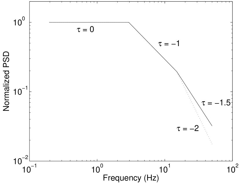
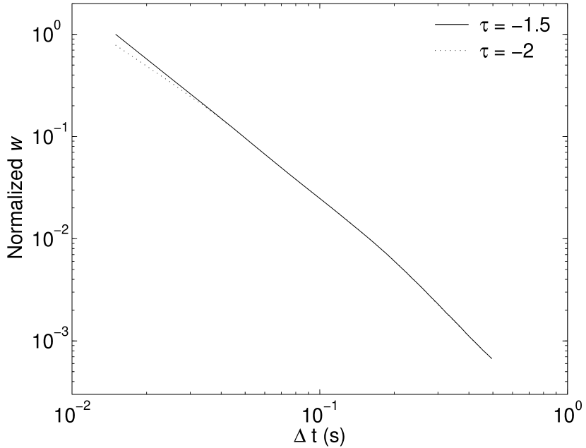
Figure 3: $w$ spectra of lightcurves with different PSD power-law indices. Left: PSDs of two lightcurves with power-law index $\tau=0$ when $f<3$ Hz, $\tau=-1$ when $f\geq 3$ and $<15$ Hz, and $\tau=-1.5$ or $-2$ when $f\geq 15$ Hz. Right: $w$ spectra of these two lightcurves. From the simulation, we can see that the frequency breaks in the PSD do not correspond to timescale cut-offs, but manifest as different slopes in the $w$ spectra.

To address the question whether $w$ spectrum may also detect the frequency breaks often seen in the PSD of the lightcurves many astrophysical sources, we simulate two lightcurves with different PSDs (using the inverse FFT method of Timmer & König, 1995). The PSD consists of power-law forms at different segments: power-law index $\tau=0$ when $f<3$ Hz, $\tau=-1$ when $f\geq 3$ and $<15$ Hz, and $\tau=-1.5$ or $-2$ when $f\geq 15$ Hz (left panel of Fig. 3). The $w$ spectra of these two lightcurves are presented in the right panel of Fig. 3. We can see that the frequency breaks in the PSD do not correspond to timescale cut-offs, but manifest as different slopes in the $w$ spectra.

In sum, the $w$ spectrum is only sensitive to the width distribution of a shot series, but insensitive to other shot parameters, such as the shot profile, shot separation distribution and shot amplitude. In particular, the $w$ spectrum is especially powerful in detecting the smallest shot width of a shot series.

3 Data Analysis

We apply the timescale analysis method to observations of a number of X-ray binaries with the Proportional Counter Array (PCA) on board Rossi X-ray Timing Explorer (RXTE). The data are screened when five PCUs are all on and the original time bin size $\delta t$ of the lightcurve is binned to 2 ms or 4 ms according to the data mode, with each segment of 50000 bins (100 s or 200 s). Because this analysis method can tolerate high level of noise, we did not avoid PCA channels 0-7, which have higher level of instrumental background. The observation IDs and other details of used data are listed in Table 1.

The top panel of Figure 4 shows the normalized $w_{s}$ spectra of five accretion BHCs, GRS 1915+105, GRO J1655-40, GX 339-4, XTE J1550-564, and Cyg X-1. All spectra show a cut-off at a timescale about 0.05 s. But for five selected NS binaries with weak magnetic field, i.e., 4U 1705-440, GS 1826-24, 4U 0614+091, 4U 1608-522, and Cyg X-2, the $w_{s}$ spectra have no obvious cut-off above $10^{-2}$ s (see the bottom panel of Fig. 4).

The energy dependent analysis is carried out for three BHC binaries: Cyg X-1, XTE J1550-564, and GRO J1655-40. All sources are at their hard state. The choice of energy bands for each observation reflects the different data mode of each observation. From Figure 5, one can see a common trend: below about 10-20 keV the cut-off timescale $\Delta t_{c}$ decreases with increasing energy, and above about 10-20 keV $\Delta t_{c}$ increases with increasing energy. An emission feature at iron K$\alpha$ line appears clearly in the energy spectra of Cyg X-1 and XTE J1550-564, and a broad peak around $\sim$ 6 keV can also be seen in their $\Delta t_{c}$ spectra. For GRO J1655-40, the Fe reflection component is very weak in the energy spectrum of this observation, and this broad peak in its $\Delta t_{c}$ spectra is also not seen.

4 Discussion

Extracting physical information from lightcurves for multi-timescale and aperiodic processes is difficult. However, it is important to study the underlying physics in high-energy processes around compact objects. The timescale analysis technique has the freedom of selecting or designing a proper statistic for a particular purpose. Our results of simulation and data analysis for accreting X-ray sources show that the proposed statistic $w$ is useful in timescale analysis of shot widths. From their $w$ spectra (the top panel of Fig. 4), we find that the BHCs have shortest shot width $\sim$ 0.05 s, consistent with that shots in BHCs have characteristic timescale $\sim$ 0.1 s, which was previously derived by a timescale analysis of power density (Li & Muraki, 2002). The fact that no short timescale cut-off appears in the $w$ spectra of NS binaries (the bottom panel of Fig. 4) is also consistent with what indicated by their timescale spectra of power density (Li & Muraki, 2002), and by Fourier spectral analysis (Sunyaev & Revnivtsev, 2000) of these systems in the hard state. The timescale analysis technique of shot width proposed in this work, like the time domain power spectrum analysis, can help us distinguish BHCs from NSs. Compared with the timescale analysis of power density spectrum, the statistic $w$ can measure more directly and sensitively the lower cut-off of shot timescale, with which we can study the energy dependence of the cut-off timescale quantitatively.

The variation timescale is usually taken as an indicator of the spatial dimensions of the underlying physical process. The remarkable result from our timescale analysis with the statistic $w$ is the energy dependent timescale cut-off of BHCs (Fig. 5) is hard to explain by a simple correspondence between the variation timescale and the radius where shots take place. The monotonic increase of the timescale cut-off with energy in the region of $E\geq 10$-20 keV is consistent with previous time domain analysis of variability in Cyg X-1 and other BHCs (e.g., Feng, Li, & Chen, 1999; Li, Feng, & Chen, 1999; Maccarone, Coppi, & Poutanen, 2000; Negoro, Kitamoto, & Mineshige, 2001), which is expected from the common understanding that hard X-rays come from inverse Compton scattering of low-energy seed photons by high-energy electrons in a hot corona (e.g., Eardley, Lightman, & Shapiro, 1975; Poutanen & Svensson, 1996; Dove et al., 1997) or hot advection-dominated accretion flow (ADAF) (e.g., Esin et al., 1998), where a shot of low energy seed photons are hardened and broadened by the Comptonization process.

A rough estimate from Figure 5 can be made to evaluate the corona size $R_{c}$ of a BHC. We assume a typical temperature of $\sim$100 keV for the hot corona at the hard spectral state. The mean free path of X-rays in corona can be considered as the corona’s spatial dimension $R_{c}$, because its optical depth is $<$ 1 from the energy spectral fitting. We assume the turning point energy $E_{0}$ at $w$ spectrum as the energy of input seed shot photons, and after $k$ times of inverse Compton scattering, the mean photon energy is increased to $E_{k}$, the timescale $\Delta t_{ck}$ of shots at energy $E_{k}$ can then be located in the $\Delta t_{c}$ spectrum. By a simple relationship of $\Delta t_{ck}=\Delta t_{c0}+k\,R_{c}/c$, where $\Delta t_{c0}$ is the turning point timescale in the $\Delta t_{c}$ spectrum and $c$ is the light speed, $R_{c}$ is then estimated. From Figure 5, the approximately derived $R_{c}$ are in order of 30, 140 and 70 $R_{s}$ (Schwarzschild radius) for Cyg X-1, XTE J1550-564 and GRO J1655-40, respectively, assuming these BHC masses are 10, 10 and 7 $M_{\odot}$ (Quirrenbach et al., 2002).

It is obvious that the general trend of timescale cut-off vs. energy in the energy region of $E\leq 10$-20 keV is opposite to that in higher energy region. We first ignore the broad peak around 6 keV in the $\Delta t_{c}$ spectrum and focus on the decreasing trend of $\Delta t_{c}$ with increasing energy at $E\leq 10$-20 keV. One probability is that shots of different energies are produced in different regions of the disk: the high energy shots are located at inner disk and low energy ones are from outer region. The turning point at $\sim$ 10-20 keV may indicate that the maximum energy of the initial shot photons, which are most probably produced at the turbulent region of the cold disk joining the hot corona, can be as high as up to $\sim$ 10-20 keV (Manmoto et al., 1996; Li, Feng, & Chen, 1999).

Another possibility to explain the $\Delta t_{c}$ spectrum at energy below the turning point is to consider the shots with energies below the turning point are produced by down-Comptonization, i.e., original shots with energy at the turning point are scattered by cold electron cloud covering the accretion disk (Zhang et al., 2000). From the top panel of figure 5 (Cyg X-1), we can see that from 11.6 keV (the turning point energy) to 2.4 keV (the lowest energy) the timescale is increased by 0.037 s. If the mean kinetic energy of cold electrons is much less than the turning point energy, about 170 times of scattering are needed for the X-ray energy increased from the turning point energy to 2.4 keV. Assuming the relationship between the increase of timescale $\Delta t$, the number of scattering $N$ and mean free path $l$ under the optically thick condition, is described by $\Delta t=lN/c$, the derived mean free path $l$ is $6.5\times 10^{6}$ cm (2.2 $R_{s}$ of Cyg X-1).

Under the above assumption that an optically thick cold electron cloud covers the initial shots (with energy at the turning point of the $\Delta t_{c}$ spectrum) located near the innermost region of the disk, we can evaluate the geometry of the cold electron cloud, from the shape of the the $\Delta t_{c}$ spectrum (top panel of fig. 5 for Cyg X-1). The distance between the location where the down-scattered photons escape to the seed shot photon region can be described as $D=\tau l$, where $\tau$ is the optical depth and equal to $\sqrt{N}$ in an optically thick system. We find that $\tau$ increases and $l$ decreases when the photon energy decreases, and consequently $D\approx 30R_{s}$ of $D$ is obtained, almost independent of the escaped photon energy. Similarly we also applied the above procedure to the data on XTE J1550-564 and GRO J1655-40. In Figure 6 we show the relationship between $D$ and the escaped photon energy.

Our calculation for Cyg X-1 also indicates that if the mean temperature of electrons is larger than 0.03 keV, the above down-Comptonization process cannot decrease the average photon energy from the turning point to below 2.4 keV. For example, if the electron temperature is 0.03 keV, after about 1000 Compton scattering the average photon energy saturates at 2.4 keV, down from the seed shot photon energy of 11.6 keV. So if the above assumed down-Comptonization scenario is true for the $\Delta t_{c}$ spectrum below the turning point, we predict that a sharp increase of timescale in the $\Delta t_{c}$ spectrum below the saturation energy, which is uniquely related to the temperature of the cold electron cloud.

Finally we examine the broad peak in the $\Delta t_{c}$ spectrum around $\sim$ 6 keV for Cyg X-1 and XTE J1550-564. It is most probably produced by the disk reflection component: reprocessed iron K$\alpha$ fluorescent photons in the cold disk irradiated by hard X-rays with energy above the $\sim$7keV iron K-edge will further broaden the shots. This interpretation is also consistent with the explanation of time delays and the behavior of the iron line (Gilfanov, Churazov & Revnivtsev, 2000; Poutanen, 2002) with frequency-resolved energy spectra (Revnivtsev, Gilfanov & Churazov, 1999). Besides producing the fluorescence iron K$\alpha$ emission, the refection also has a strong component at energies above 10 keV, which may contribute to the increase of shot width above the tuning point in addition to the up-Comptonization process we discussed above.

Table 1: RXTE/PCA observations Used

	Object	OBS ID	Band (keV)	Used at
	4U 1705-440	20073-04-01-00	3-20	Fig. 4
	GS 1826-24	30054-04-01-00	3-20	Fig. 4
Neutron Star	4U 0614+091	30054-01-01-01	3-7	Fig. 4
X-ray Binaries	4U 1608-522	30062-01-01-04	3-7	Fig. 4
	Cyg X-2	30418-01-01-00	2-5	Fig. 4
	Cyg X-1	10236-01-01-03	2-67	Fig. 4
	Cyg X-1	40100-01-01-00	2-61	Fig. 5
	GRS 1915+105	20402-01-05-00	2-5	Fig. 4
Black Hole	GRO J1655-40	20402-02-25-00	2-5	Fig. 4
X-ray Binaries	GX 399-4	20181-01-01-00	7-22	Fig. 4
	XTE J1550-564	30191-01-14-00	2-7	Fig. 4
	XTE J1550-564	30191-01-17-00	2-60	Fig. 5
	GRO J1655-40	10255-01-04-00	2-50	Fig. 5

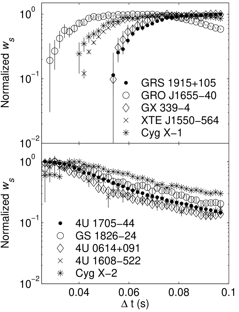
Figure 4: Timescale spectra of $w_{s}$ for BHC and NS binaries. Top: Black hole binary candidates; Bottom: weakly magnetized neutron star binaries. All BHC samples show cut-offs below about 0.05 s, contrary to NS binaries.

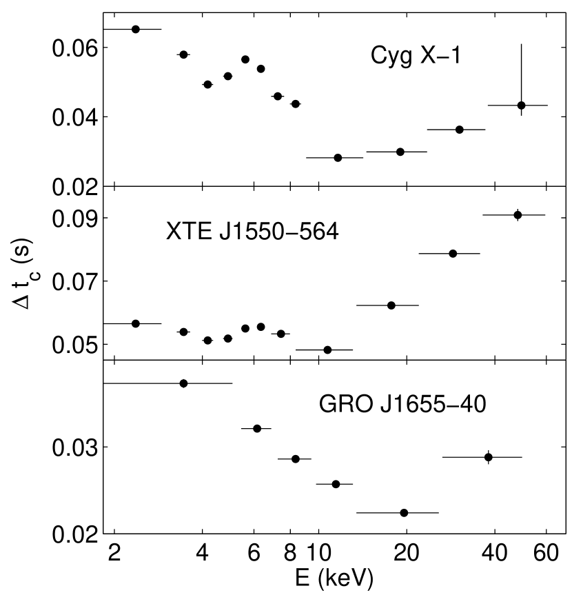
Figure 5: Timescale cut-off vs. energy for three BHCs.

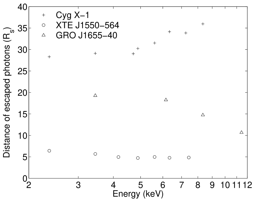
Figure 6: Transportation distance of photons from the seed shots location to the surface of the cold electron cloud.

References

- Dove et al. (1997) Dove, J.B., Wilms, J., Maisack, M.M., & Begelman, M.C. 1997, ApJ, 487, 759
- Eardley, Lightman, & Shapiro (1975) Eardley, D.M., Lightman, A.P., & Shapiro, S. 1975, ApJ, 199, L153
- Esin et al. (1998) Esin, A.A., Narayan, R., Cui, W., Grove, J.E., & Zhang, S.N. 1998, ApJ, 505, 854
- Feng, Li, & Chen (1999) Feng, Y.X., Li, T.P., & Chen, L. 1999, ApJ, 514, 373
- Gilfanov, Churazov & Revnivtsev (2000) Gilfanov, M., Churazov, E., and Revnivtsev, M. 2000, MNRAS, 316, 923
- Li, Feng, & Chen (1999) Li, T.P., Feng, Y.X., & Chen, L. 1999, ApJ, 521, 789
- Li (2001) Li, T.P. 2001, Chin. J. Astron. Astrophys., 1, 313 (astro-ph/0109468)
- Li & Muraki (2002) Li, T.P., & Muraki, Y. 2002, ApJ, 578, 374
- Lochner, Swank, & Szymkowiak (1991) Lochner, J.C., Swank, J.H., & Szymkowiak, A.E. 1991, ApJ, 375, 295
- Manmoto et al. (1996) Manmoto, T., Takeuchi, M., Mineshige, S., Matsumoto, R., & Negoro, H. 1996, ApJ, 464, L135
- Meekings et al. (1984) Meekins, J.F., Wood, K.S., Hedler, R.L., Byram, E.T., Yentis, D.J., Chubb, T.A., & Friedman, H. 1984, ApJ, 278, 288
- Maccarone, Coppi, & Poutanen (2000) Maccarone, T.J., Coppi, P.S., & Poutanen, J. 2000, ApJ, 537, L107
- Miyamoto et al. (1988) Miyamoto, S., Kitamoto, S., Mitsuka, K., & Dotani, T. 1988, Nature, 336, 450
- Miyamoto et al. (1992) Miyamoto, S., Kitamoto, S., Iga, S., Negoro, H., & Terada, K. 1992, ApJ, 391
- Negoro, Miyamoto, & Kitamoto (1994) Negoro, H., Miyamoto, S., & Kitamoto, S. 1994, ApJ, 423, L127
- Negoro, Kitamoto, & Mineshige (2001) Negoro, H., Kitamoto, S., & Mineshige, S. 2001, ApJ, 554, 528
- Nolan et al. (1981) Nolan, P.L., et al. 1981, ApJ, 246, 494
- Oda et al. (1971) Oda, M., Gorenstein, P., Gursky, H., Kelloge, E., Schreier, E., Tananbaum, H., & Giacconi, R. 1971, ApJ, 166, L1
- Oda (1977) Oda, M. 1977, Space Sci. Rev., 20, 757
- Poutanen (2002) Poutanen, J. 2002, MNRAS, 332, 257
- Poutanen & Svensson (1996) Poutanen, J., & Svensson, R. 1996, ApJ, 470, 249
- Quirrenbach et al. (2002) Quirrenbach, A., Frink, S. & Tomsick, J. 2002, Science with the Space Interferometry Mission, Project summaries, 33
- Revnivtsev, Gilfanov & Churazov (1999) Revnivtsev, M., Gilfanov, M., and Churazov, E. 1999, A&A, 347, L23
- Sunyaev & Revnivtsev (2000) Sunyaev, R., & Revnivtsev, M. 2000, A&A, 358, 617
- Sutherland, Weisskopf & Kahn (1978) Sutherland, P.G., Weisskopf, M.C., & Kahn, S.M. 1978, ApJ, 219, 1029
- Tanaka & Lewin (1995) Tanaka, Y., & Lewin, W. H. G. 1995, in X-Ray Binaries, ed. W. H. G. Lewin, J. VAN Paradijs, & E. P. J. Heuvel (Cambridge: Cambridge Univ. Press), 126
- Terrel (1972) Terrel, N.J. 1972, ApJ, 174, L35
- Timmer & König (1995) Timmer, T. and König, M 1995, A&A, 300, 707
- van der Klis (1995) van der Klis, M. 1995, in X-Ray Binaries, ed. W. H. G. Lewin, J. VAN Paradijs, & E. P. J. Heuvel (Cambridge: Cambridge Univ. Press), 252
- Zhang et al. (2000) Zhang, S.N., Cui, W., Chen, W., Yao, Y., Zhang, X.L., Sun, X.J., Wu, X.B., and Xu, H.G. 2000, Science, 287, 1239