The Sky Polarization Observatory (SPOrt)

Abstract

SPOrt is an ASI–funded experiment specifically designed to measure the sky polarization at 22, 32 and 90 GHz, which was selected in 1997 by ESA to be flown on the International Space Station. Starting in 2006 and for at least 18 months, it will be taking direct and simultaneous measurements of the Stokes parameters Q and U at 660 sky pixels, with ${\rm FWHM}=7^{\circ}$. Due to development efforts over the past few years, the design specifications have been significantly improved with respect to the first proposal. Here we present an up–to–date description of the instrument, which now warrants a pixel sensitivity of 1.7 $\mu$K for the polarization of the cosmic background radiation, assuming two years of observations. We discuss SPOrt scientific goals in the light of WMAP results, in particular in connection with the emerging double–reionization cosmological scenario.

, , , , , , , , , , , , , , , , , , , , , , , , , , , , , ,

1 Introduction

The last decade of the past century has seen a number of great achievements in observational cosmology. Among them, the assessment of the nature of the cosmic microwave background radiation (CMBR), by COBE (Mather et al. 1990, 1999), and the detection of its tiny temperature fluctuations (Smoot et al. 1992; Bennett et al. 1996), providing a sound confirmation of the gravitational instability picture. After COBE, a number of ground and balloon experiments (see, e.g., De Bernardis et al. 2000, Hanany et al. 2000 for a review), together with the ongoing WMAP mission (Bennett et al. 2003), extended the measured angular spectrum of temperature fluctuations up to $l\simeq 800$. By fitting model predictions to these measurements, the multi–dimensional parameter space of available cosmological models was significantly constrained.

The main target of further analysis was clearly polarization. Besides conveying independent information on the cosmological model, so as to remove residual degeneracies between various parameters, large angle polarization data allow to explore the thermal history of the Universe at low redshift, in the epoch when primeval fluctuations gradually turned into today’s systems and objects. Upper limits to the polarization signal had been put by ground experiments (see, e.g., Keating et al. 2001; Hedman et al. 2002), while DASI (Kovac et al. 2002) claimed a detection with significance of $4.9\sigma$ on angular scales $\sim 0.5^{o}$.

The entry into the new century of CMBR exploration was however set by WMAP detecting a clear signal of TE correlation at large angular scales (Kogut et al. 2003). This was much more than an aid to remove parameter degeneracies. Its intensity carried unexpectedly important information on the history of our Universe, operating a radical selection among reionization scenarios.

This finding makes the SPOrt experiment quite timely. This experiment, fully funded by the Italian Space Agency (ASI), was proposed to the European Space Agency (ESA) in 1997 to put a polarimeter onboard the International Space Station (ISS). Its frequency range (22–90 GHz) and angular resolution (${\rm FWHM}=7^{\circ}$), together with an almost full–sky coverage, are optimal to search for CMBR polarization on large angular scales. This strategy has now received an unexpectedly strong support by the first–year WMAP release, which favours values of the Universe optical depth $\tau\sim 0.17$.

Such high values need a confirmation, which shall come first by further WMAP releases. An independent confirmation, based on an instrument devoted to polarization and operating independently from anisotropy, will then be allowed by the SPOrt experiment. It should be stressed that a safe assessment on a so large $\tau$ is not only quantitatively relevant, but changes our views on the history of cosmic reionization and on the very epoch when the first objects populated the Universe. Besides allowing to measure $\tau$, large angle polarization will also put new constraints on the nature of Dark Energy (DE), which determines the relation between time and scale factor in the epoch when reionization occurred.

Only full sky experiments, based on space, can provide information on large angular scale polarization, ground based or balloon experiments being intrinsically unable to access such scales.

In the light of such considerations, here we report on the present advancement of the SPOrt experiment, on the technical aspects of the polarimeter we shall fly and on the physics we expect to explore through its observations.

The plan of the paper is as follows: Sect. 2 reviews large–scale CMBR polarization theory as well as the current scenario, including foregrounds; Sect. 3 describes the SPOrt experiment, with special emphasys on its technological and design aspects; Sect. 4 is focused on the main physics results SPOrt is expected to provide, compared to WMAP. The conclusion are summarised in Sect. 5.

2 Scientific targets: theory and current scenario

2.1 Anisotropy and polarization: definitions

SPOrt aims at measuring the polarization of CMBR. Quite in general, to define the properties of linearly polarized radiation coming from a sky direction $\hat{n}$, we make use of a basis $(\hat{e}_{1},\hat{e}_{2})$, in the plane perpendicular to $\hat{n}$, to define the $2\times 2$ tensor $I_{ij}=\langle E_{i}E_{j}\rangle/4\pi c$ ($E_{i}$ are components of the electric field vector $\hat{E}$, perpendicular to $\hat{n}$). The total intensity of the radiation from the direction $\hat{n}$ is then the tensor trace $I=I_{11}+I_{22}$. By angle averaging, we obtain the average radiation intensity $\bar{I}$.

This average value ought to be subtracted from the signal, to detect the main CMBR features. We therefore replace $I_{ij}$ by the tensor $\Delta_{ij}={I_{ij}/{\bar{I}}}-\delta_{ij}/2$. Its components are directly related to the temperature anisotropies and the Stokes parameters accounting for linear polarization, as follows:

$$T=(\Delta_{11}+\Delta_{22})/4~{},~{}Q=(\Delta_{11}-\Delta_{22})/4~{},~{}U=\Delta_{12}/2.$$ (1)

$Q$ and $U$ depend on the basis $(\hat{e}_{1},\hat{e}_{2})$. If such basis is rotated by an angle $\psi$, so that ${\hat{e}_{1}}^{\prime}=\cos\psi\ {\hat{e}_{1}}+\sin\psi\ {\hat{e}_{2}}$ and ${\hat{e}_{2}}^{\prime}=-\sin\psi\ {\hat{e}_{1}}+\cos\psi\ {\hat{e}_{2}}$, the Stokes parameters change into $Q^{\prime}=\cos 2\psi\ Q+\sin 2\psi\ U$, $U^{\prime}=-\sin 2\psi\ Q+\cos 2\psi\ U$. According to Tegmark & de Oliveira–Costa (2001), it is then convenient to define a 3–component quantity

$$\mathbf{D}\equiv(T,Q,U)$$ (2)

which transforms into

$$\mathbf{D^{\prime}}=\mathbf{R}(\psi)\mathbf{D}~{},$$ (3)

when the basis is rotated by $\psi$; here

$$\mathbf{R}(\psi)=\left(\matrix{1&0&0\cr 0&\cos 2\psi&\sin 2\psi\cr 0&-\sin 2\psi&\cos 2\psi\cr}\right)$$ (4)

is a $3\otimes 3$ matrix.

2.1.1 Angular Power Spectra

$T$, $Q$ and $U$ depend on the sky direction $\hat{n}$. From them we obtain angular power spectra (APS), by expanding on suitable spherical harmonics. The spherical harmonics currently used to expand anisotropies ($T$) are however inappropriate for polarization, as the combinations $Q\pm iU$ are quantities of spin $\pm 2$ (Golberg et al. 1967). In this case, one makes use of the spin–weighted harmonics $\,{}_{\pm 2}Y_{l}^{m}$ (Zaldarriaga & Seljak 1997)

$$\begin{array}[]{rll}T(\hat{n})&=&\sum_{lm}a_{T,lm}Y_{lm}(\hat{n})\\ (Q+iU)(\hat{n})&=&\sum_{lm}a_{+2,lm}\;{}_{+2}Y_{lm}(\hat{n})\\ (Q-iU)(\hat{n})&=&\sum_{lm}a_{-2,lm}\;{}_{-2}Y_{lm}(\hat{n}).\\ \end{array}$$ (5)

In order to relate CMBR polarization to its origin, instead of using the Stokes parameters $Q$ and $U$, it is more convenient to describe linear polarization through two suitable scalar quantities $E$ and $B$ (see: Seljak & Zaldarriaga 1997 and Kamionkowski et al. 1997a, who give a slightly different notation). Theory provides direct predictions on such quantities and the treatment in terms of $E$ and $B$ takes full account of the spin–$2$ nature of polarization. Their scalar harmonics coefficients are related to $a_{\pm 2,lm}$ by the linear combinations $a_{E,lm}=-(a_{2,lm}+a_{-2,lm})/2$ and $a_{B,lm}=(a_{2,lm}-a_{-2,lm})/2i$.

These combinations transform differently under parity. Thanks to that, just four angular spectra $C_{Yl}$ ($Y=T$, $E$, $B$ and $TE$) characterize fluctuations, if they are Gaussian. These APS are the transforms of the autocorrelations of $T$, $E$ and $B$ and the cross–correlation between $E$ and $T$; invariance under parity grants the vanishing of the cross–correlations between $B$ and any other quantity, and the related APS. More in detail, such APS are defined as follows:

$$\begin{array}[]{lllclll}\langle a_{T,lm}^{*}a_{T,lm^{\prime}}\rangle&=&\delta_{m,m^{\prime}}C_{Tl};&&\langle a_{E,lm}^{*}a_{E,lm^{\prime}}\rangle&=&\delta_{m,m^{\prime}}C_{El}\\ \langle a_{B,lm}^{*}a_{B,lm^{\prime}}\rangle&=&\delta_{m,m^{\prime}}C_{Bl};&&\langle a_{T,lm}^{*}a_{E,lm^{\prime}}\rangle&=&\delta_{m,m^{\prime}}C_{TEl}.\end{array}$$ (6)

In order to fit data with models, one must also be able to invert these relations, working out signal correlations from APS. This operation can be fairly intricate, because of the complex properties of spherical harmonics. One can start the procedure by defining the following functions:

$$F_{1,lm}(\theta) = 2\sqrt{\frac{(l-2)!(l-m)!}{(l+2)!(l+m)!}}\left\{\left[\frac{m^{2}-l}{\sin^{2}\theta}-\frac{l(l-1)}{2}\right]\cdot\right.$$

$$\left.P_{l}^{m}(\cos\theta)+(l+m)\frac{\cos\theta}{\sin^{2}\theta}P_{l-1}^{m}(\cos\theta)\right\}$$

$$F_{2,lm}(\theta) = 2\sqrt{\frac{(l-2)!(l-m)!}{(l+2)!(l+m)!}}\cdot\frac{m}{\sin^{2}\theta}\cdot\big{[}-(l-1)\cdot$$ (7)

$$\cos\theta P_{l}^{m}(\cos\theta)+(l+m)P_{l-1}^{m}(\cos\theta)\big{]}.$$

Then, simple but lengthy calculations provide relations, similar to the equation

$$\langle T(1)~{}T(2)\rangle=\sum_{l}{\frac{2l+1}{4\pi}}C_{Tl}P_{l}(\cos\alpha_{12})$$ (8)

($\alpha_{12}$ is the angle between the directions 1 and 2), relating fluctuations to spectra, for Stokes parameters and their correlations. Let us remind that the l.h.s. of Eq. (8) prescribes an averaging operation which, in principle, is an ensemble average. To work out such function from data, the average is taken on all pairs of sky directions with angular separation $\alpha_{12}$.

The relations analogous to Eq. (8), for the Stokes parameters, are simpler if the basis vector $\hat{e}_{1}$ is aligned with the line connecting the points 1 and 2. There they read

$$\langle Q(1)Q(2)\rangle = \sum_{l}{2l+1\over 4\pi}[C_{El}F_{1,l2}(\alpha_{12})-C_{Bl}F_{2,l2}(\alpha_{12})]$$

$$\langle U(1)U(2)\rangle = \sum_{l}{2l+1\over 4\pi}[C_{Bl}F_{1,l2}(\alpha_{12})-C_{El}F_{2,l2}(\alpha_{12})]$$

$$\langle T(1)Q(2)\rangle = -\sum_{l}{2l+1\over 4\pi}C_{TEl}F_{1,l0}(\alpha_{12})$$

$$\langle T(1)U(2)\rangle = 0.$$ (9)

For a generic basis, such relations are more complicated (Ng & Liu 1999). Owing to their definition and to Eq. (3), however, it is evident that the correlation are components of the $3\otimes 3$ matrix $\langle D_{i}D_{j}\rangle$, which transforms as follows:

$$\langle D_{i_{1}}^{\prime}D_{i_{2}}^{\prime}\rangle=R_{i_{1},j_{1}}(\psi_{1})\langle D_{j_{1}}D_{j_{2}}\rangle R_{i_{2},j_{2}}(\psi_{2})$$ (10)

with $\mathbf{R}$$(\psi)$ defined in Eq. (4); $\psi_{1,2}$ are the rotation angles to put the local polar basis in 1,2 along the great circle connecting the pair. Making use of these transformations, we can pass from the priviledged basis, where Eqs. (2.1.1) hold, to the generic basis needed for observational or modellization aims.

When real data are considered, an extra complication cannot be avoided, as detected signals suffer from both the finite resolution of antennae and pixilation effects. The total result is an effective reduction of the actual power at a given multipole, and the measured APS become

$$C_{Y,l}^{meas}=C_{Y,l}|_{s}W_{l}|^{2}$$ (11)

with

$${}_{s}W_{l}=b_{pix,l}\,{}_{s}B_{l}$$ (12)

where $b_{pix,l}$ is the spherical harmonic decomposition of the pixel window function, and ${}_{s}B_{l}$ is the beam window function. This writes

$$_{s}B_{l}=\exp[-(l(l+1)-s^{2})\sigma^{2}/2],$$ (13)

where $\sigma={\rm FWHM}/\sqrt{8\ln 2}$ for Gaussian beams and $s=2$ for polarization, whereas $s=0$ for anisotropy (Ng & Liu 1999). The rms polarization $P_{\mathrm{rms}}$ measured over a finite–resolution map is then given by

$$P_{\mathrm{rms}}^{2}=\sum_{l\geq 2}\frac{2l+1}{4\pi}C_{Pl}\,{}_{2}W_{l}^{2},$$ (14)

where

$$C_{Pl}=C_{El}+C_{Bl}.$$ (15)

When $Q$ and $U$ maps are available one can also use $P_{\mathrm{rms}}^{2}=Q^{2}_{rms}+U^{2}_{rms}$).

As an example, let us consider an instrument with a FWHM aperture of $7^{\circ}$. In this case the reduction caused by a factor $(_{2}W_{l}/b_{pix,l})^{2}$ is $e^{2}$ for $l\simeq 27$. It is then clear why, with such an aperture, it makes sense to explore spherical harmonics up to $l=30$. Let us further recall that, in order to obtain an optimal exploitation of the signal, it is convenient to set pixels with centres at a distance $\sim\rm{FWHM}/2$.

2.1.2 Small sky areas and non–Gaussian signals

The treatment of the previous subsection can be simplified, when a small patch of the sky is considered, so that the celestial sphere can be treated as flat (Seljak 1997). Then the spin–weighted harmonic expansions (5) reduce to Fourier expansions in the $(\theta_{x},\theta_{y})$ plane:

$$Y(\vec{l})=N_{\rm pix}^{-1}\sum_{k}\exp(-i\vec{l}\cdot\vec{\theta}_{k})Y(\vec{\theta}_{k})~{};$$ (16)

here $N_{\rm pix}$ is the number of pixels, and $Y$ stands for either $Q$ or $U$. Passing to $E$ and $B$ is also simpler, as

$$E({\vec{l}}) = Q({\vec{l}})\cos(\phi_{\vec{l}})+U({\vec{l}})\sin(\phi_{\vec{l}})$$

$$B({\vec{l}}) = -Q({\vec{l}})\sin(\phi_{\vec{l}})+U({\vec{l}})\cos(\phi_{\vec{l}})$$ (17)

$\phi_{\vec{l}}$ being the angle between ${\vec{l}}$ and the $\theta_{x}$ axis. From the expansion coefficients, the APS can be recovered and read

$$C_{Yl}=\Omega\left\langle Y(\vec{l})Y^{*}(\vec{l})\right\rangle\mathbf{.}$$ (18)

Here $\Omega$ is the size of the sky patch and the average $\langle\rangle$ is to be performed over those $\vec{l}$ having magnitude close to $l$. These spectral components, referring to the portion of the sky we consider, are local and can depend on the setting of such portion.

When dealing with foregrounds, which are non–Gaussian, APS can still be useful to evaluate their contamination to the CMBR signal. In such a case, an angle averaging should be explicitly performed. This amounts to summing upon $m$ and dividing by $2l+1$. Eqs. (2.1.1) should not be used, because of the phase coherence of harmonic amplitudes. Furthermore, one should carefully distinguish between local and global APS. Foreground subtraction ought to be performed using local APS; in principle locality should be enhanced as much as data uncertainties allow, in order to perform correct subtractions on small angular scales.

It was not recognized for some time that, by expanding the polarized intensity $\Pi=\sqrt{Q^{2}+U^{2}}$ in spherical harmonics, a further spectrum, $C_{\Pi l}$, is constructed. As first noted in Tucci et al. (2002) $C_{\Pi l}$ conveys an information distinct from $C_{Pl}$. In particular, $C_{\Pi l}$ provides an incomplete information, since it does not include the polarization direction; for instance, it cannot be used to build simulated polarization maps, and cannot account for beam–depolarization effects. However, it is still useful when studying the emission of Galactic foregrounds at low frequency ($\leq 2$ GHz), where $C_{El}$ and $C_{Bl}$ can be affected by Faraday rotation, whereas $C_{\Pi l}$ turns out to be quasi–independent of it (Tucci et al. 2002), and can be safely extrapolated to higher frequencies.

2.2 Origins of anisotropies and polarization of the CMBR

Photons undergoing Thomson scattering become polarized. In the presence of uniform and isotropic electron and photon distributions, however, angular averaging smears out polarization. To preserve some of it, not only must the photon distribution be anisotropic, but anisotropy must have a quadrupole component. Until photons and baryons are tightly coupled so as to form a single fluid, any quadrupole in the photon distribution is erased; accordingly, all scales entering horizon before recombination develop a quadrupole only after decoupling begins, so that photon and baryon inhomogeneities are out of phase.

When photons have acquired a mean–free–path of the order of fluctuation sizes, therefore, quadrupole anisotropies arise. Such a long mean–free–path, however, also means that the optical depth $\tau$ of baryonic materials is approaching unity (from above) and more and more photons are unscattered until present. However, only the restricted fraction of photons that still undergo a late scattering, can acquire polarization. Therefore, primary polarization is small both because quadrupole is small and because few photons are scattered after it arises. Quadrupole (and, hence, polarization) turns however higher on scales entering recombination with larger dipole, i.e. in the kinetic stage. The number of photons scattered decreases further for scales entering the horizon after recombination, where the polarization degree rapidly fades with scale increase.

All these effects can be followed in detail by numerical linear codes, like CMBFAST, able to compute the amount of polarization produced on each scale as a function of the parameters of the underlying cosmological model. The information that the tiny polarization signal carries can therefore help to reduce any parameter degeneracies that the stronger anisotropy signal cannot resolve. In particular, the detailed history of recombination, occurring at redshifts $z\sim 10^{3}$, can be inspected through these signals.

However, it is easy to see that the horizon scale at recombination occupies an angular scale $\sim 10^{-2}$ radians, on the celestial sphere. Accordingly, the primary polarization spectrum can be expected to peak at $l\sim 10^{2}$–10³ and to be negligible at $l<30$, those $l$’s we can inspect if ${\rm FWHM}\simeq 7^{\circ}$. The above inspection is therefore precluded to the SPOrt experiment.

The polarization signal SPOrt aims at detecting must be related to later events, when the scales entering the horizon subtended angles $\sim 7^{\circ}$ or were even larger than so. Should the Universe be filled with neutral gas from recombination to now, no such polarization could be expected. It is known, on the contrary, that diffuse baryonic materials, today, are almost completely ionized. But this could not be enough: baryonic materials are so diluted, today, that the scattering time for CMBR photons $t_{s}\simeq 4.45\cdot 10^{18}\Omega_{b}^{-1}h^{-2}$s ($h$: Hubble parameter in units of 100 km/s/Mpc) widely exceeds the Hubble time $t_{H}=3.09\cdot 10^{17}h^{-1}$s. Hence, secondary polarization can arise only if reionization is early enough not to be spoiled by baryon dilution.

Let us therefore extrapolate these figures to the past: while $t_{s}\propto a^{3}$ ($a$: the scale factor), the dependence of $t_{H}$ on $a$ depends on the model. Numerical computations are avoided by assuming an expansion regime dominated by ordinary non–relativistic matter, as in a standard CDM model. Then an ionized Universe is opaque ($\tau=1$) to CMBR at $z>z_{op}\simeq 5\,(\Omega_{b}h)^{-2/3}$. If $\Omega_{b}h^{2}\leq 0.022$, as from standard BBNS limits (see Dolgov 2002 for a recent review), and $h\simeq 0.5$, we obtain $z_{op}>64$. The redshift range where reionization may have occurred ($z_{ri}$) is safely below such $z_{op}$. A standard CDM model disagrees with data, but no reasonable cosmology allows a substantial reduction of $z_{op}$. A full re–scattering of CMBR at low redshift is therefore almost excluded, but the opacity $\tau$ can be non–neglegible if $z_{ri}$ is not lower than $\sim 8$–10. In turn, this may cause secondary polarization.

2.3 Relevance of secondary polarization

Let us briefly remind which kind of physics is explored through $\tau$ measurements and, hopefully, through a more sophisticated analysis, leading to estimates of $z_{ri}$ and other related parameters. They could shed new light on (i) the cosmic reionization history and the physics of systems causing it; (ii) the expansion laws during reionization and the cosmic substance ruling the expansion.

Good reviews on point (i) were provided by Loeb & Barkana (2001), Shapiro (2001), Maselli et al. (2003) and Haiman (2003). Most studies, assuming the flat $\Lambda$–dominated concordance model ($\Omega_{m}=0.3$, $h=0.7$), until recently converged in setting $z_{ri}$ in the interval 8–10 and suggested that hydrogen ionized then and remained such until now. Reionization was attributed to radiation produced by metal–free star formation in early galaxies, whose effects depend on several parameters, as the photon escape fraction $f_{esc}$ and the slope of the Salpeter Initial Mass Function (IMF). Among the limits that such theories must fulfil is that helium, at variance from hydrogen, reionized much more recently. However, although leaving all parameters vary in the widest possible range, $z_{ri}$ values above 10 had not been envisaged. Other possible sources of reionization had been identified in AGN (Ricotti & Ostriker 2003 and reference therein) as well as exotic sources like decaying heavy sterile neutrinos (see Hansen & Haiman 2003).

These predictions were strengthened by Miralda–Escudé (2003) finding that, if the ionizing flux observed today is extrapolated to high $z$, the photon flux is able to reionize the cosmic hydrogen at $z_{ri}\sim 8$–10 and $\tau\simeq 0.08$. Furthermore Djorgovski et al. (2001) and Becker et al. (2001) reported observations of QSO’s at $z>5$, showing an increase of the Ly$\alpha$ forest opacity when $z$ goes from 5 to 6. Becker et al. (2001) also found Gunn–Peterson effect in one QSO at $z\simeq 6.3$. These data confirmed that a fraction of neutral hydrogen was present, in the intergalactic medium, at $z\sim 6$. (It must be however reminded that these very authors warned the reader against an immediate conclusion that $z_{ri}\simeq 6$.) Let us also add that Bullock et al. (2000) revived the idea of the excess of galactic satellites, that N–body simulations predict, by considering the slowing down of baryon accretion on small velocity lumps after $z_{ri}$. Their analysis apparently leads to requiring $z_{ri}<10$, at least for $\Lambda$CDM cosmologies.

Assuming an (almost) immediate and complete reionization after $z_{ri}$, in Fig. 1 we plot how $\tau$ depends on $z_{ri}$ itself, in various models, assuming $\Omega_{b}h^{2}=0.02$. A larger $\tau$ arises in flat models with low $\Omega_{m}$, but $\tau>0.08$ can hardly be reconciled with $z_{ri}<10$ while, for the aforementioned range of $z_{ri}$, the range of $\tau$ values lies typically below 0.05.

Such a satisfactory self–consistent picture has been put in severe danger by the recent WMAP release. Using their first–year observation of $C_{TEl}$ at low $l$ values, Kogut et al. (2003) estimate that, independently from any model assumption, $\tau=0.17\pm 0.04$. However, Spergel et al. (2003) comment that the low value of the quadrupole anisotropy and, in general, the rather low values of $C_{Tl}$ at $l<10$ disfavour very high $\tau$ value, as reionization should enhance large angular scales anisotropies (see, however, Efstathiou 2003). In fact, once a concordance model is assumed, the likelihood distribution is quite flat towards lower $\tau$ values and decreases just of 0.05 as $\tau$ shifts from 0.19 to 0.11.

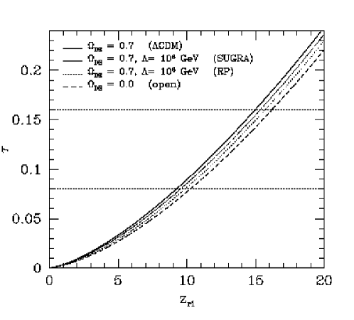
Figure 1: Opacity $\tau$ as a function of the reionization redshift, assuming instantaneous reionization at $z_{ri}$. Horizontal lines refer to $\tau$ values 0.08 and 0.16. For $\tau>0.16$ reionization must have occurred at $z_{ri}>15$, almost independently of the model.

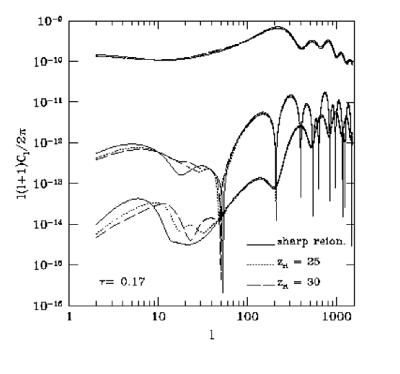
Figure 2: Dependence of angular power spectra (in K²) on model reionization histories.

Bearing in mind all these reserves and also the fact that, at the 3–$\sigma$ level, $\tau\sim 0.05$ is still consistent with observations, if we leave apart any theoretical bias, we must also accept that, e.g., a value of $\tau\sim 0.25$ is no longer excluded by the best observations now avaliable.

Such findings immediately reopened the theoretical discussion on the reionization physics. Values of $\tau\sim 0.17$ were soon found to be compatible with galaxy formation simulations by Ciardi et al. (2003), with reionization caused by stars in galaxies with total masses $\sim 10^{9}$–$10^{10}M_{\odot}$, assuming a (moderately) top–heavy Salpeter IMF, a high stellar production of ionizing photons, and a fairly high $f_{esc}\simeq 0.05$. These values are however hardly compatible with Gunn–Peterson effect findings.

A more speculative perspective becomes however more realistic in the light of high $\tau$ values: reionization might have occurred twice. Models where this occurred have been proposed by Cen (2003), Wyithe et al. (2003) and Sokasian et al. (2003). A redshift interval $\Delta z\simeq 3$, when $H$ is only partially ionized, should have elapsed between the two reionization stages. Temporary recombination might be due to feedback by SNe reducing star formation efficiency (see, e.g., Scannapieco et al. 2000, Madau et al. 2001); otherwise, a similar SNe action, concentrated in suitable spatial volumes, caused a partial temporary recombination in regions where QSO with Gunn–Peterson effect have been seen.

Figure 3: Likelihood distributions for the simultaneous determination of reionization redshift $z_{ri}$ and ionization rate $x_{e}$ in models with fixed $\tau=0.17$; the left (right) panel corresponds to a $7^{\circ}$–pixel noise $\sigma_{\rm pix}=2\,\mu$K (0.5$\,\mu$K).

Within this context, let us remind that cosmological models with equal $\tau$, but different reionization histories, predict different CMBR anisotropy and polarization. This is shown, first of all, in Fig. 2, where APS, for a fixed $\tau$ value, but different reionization histories, are shown. The other parameters of this spatially flat model are $\Omega_{b}h^{2}=0.02$, $\Omega_{m}=0.3$, $h=0.7$.

Besides the case of a sharp reionization, taking place at the nearest possible redshift, we also consider reionizations starting at larger $z_{ri}$, followed by a single zero–ionization interval, suitably set to recover the fixed $\tau$ value. Notice, in particular, that the high–$l$, apparently, does not depend on $z_{ri}$, while the shift, at low $l$, is quite significant.

The plot in Fig. 2 was made with a suitable generalization of the CMBFAST program. Using the techniques described in Sect. 4.1, we can estimate likelihood distributions and see that the differences shown in Fig. 2 enable us to set significant constraints on cosmological parameters, already with a sensitivity close to SPOrt’s.

In Fig. 3 (see Colombo et al. 2003; Mainini et al. 2003), we consider two models with $\tau=0.17$, either due to full reionization ($x_{e}=1.0$) arising at the nearest possible redshift ($\simeq 17$) or to a reionization with constant $x_{e}=0.6$, again since the nearest possible redshift ($\simeq 24$); the other model parameters are as in Fig. 2.

In both plots 1– and 2–$\sigma$ confidence curves for the simultaneous determination of $x_{e}$ and $z_{ri}$ are shown, by solid and dashed lines, respectively. Such curves are obtained by averaging over 1000 realizations of each model. The plots are also crossed by constant–$\tau$ curves corresponding to three $\tau$ values. The l.h.s. (r.h.s.) plot corresponds to a pixel noise $\sigma_{\rm pix}=2\,\mu$K (0.5$\,\mu$K), where the pixel size is about $7^{\circ}$.

A first observation is that $\tau$ is more easily determined than $x_{e}$ and $z_{ri}$, separately. Furthermore, it is clear that the level of pixel noise that SPOrt is likely to achieve ($\sigma_{\rm pix}\simeq 2\,\mu$K) is just marginal to distinguish between the two models. If $\sigma_{\rm pix}=0.5\,\mu$K, instead, at the 1–$\sigma$ level, confidence curves are disconnected and have just a marginal intersection at the 2–$\sigma$ level. The capability of SPOrt to distinguish reionization histories cannot be excluded and depends on the model realization in the real Universe.

In principle, however, the aforementioned figures show that an analysis of CMBR polarization data is an excellent probe into the reionization pattern of the Universe and, therefore, on birth, evolution and death of early starlike objects.

Let us now come to the point (ii): in shaping polarization spectra, the nature of the Dark Energy (DE) component of the Universe plays a role. For the sake of example, in Fig. 4 we show the $l$–dependence of $C_{TEl}$ for $l$ up to 40. In all plots $\Omega_{b}=0.05$, $h=0.7$, $\Omega_{m}=0.3$, while the solid (dashed) curve refers to $\tau=0.14$ (0.20). In all plots the spectra of a $\Lambda$CDM model are shown, together with the spectra for models where DE is due to a scalar field $\phi$, self–interacting through a Ratra–Peebles (1988, RP hereafter) power–law potential $V(\phi)=\Lambda^{\alpha+4}/\phi^{\alpha}$. [In some figure of this paper we consider also SUGRA potentials $V(\phi)=(\Lambda^{\alpha+4}/\phi^{\alpha})\exp(4\pi G\phi^{2})$, Brax & Martins 1999, 2000]. The three plots differ for the choice of the energy scale $\Lambda$ and $\lambda=\log_{10}(\Lambda/{\rm GeV})$. The differences between $\Lambda$CDM and RP models, already significant for $\lambda=2$, become huge for $\lambda=14$, where the first correlation peak has even negative values.

The impact of DE nature can be even better appreciated in Fig. 5, where we plot the likelihood distributions on $\Lambda$, as obtainable when artificial data built from RP models, with the $\lambda$ scale indicated in top of each frame, are “observed”. Here again, the techniques described in Sect. 4.1 have been used. In the plots, the histograms report the distribution of the peak likelihood, as obtained from 1000 realizations of each model. The solid curves, instead, are the likelihood distributions, as obtained by averaging over all realization. Upper (lower) plots refer to a pixel noise of 0.2$\,\mu$K (2.0$\,\mu$K).

While, for the unlikely model $\lambda=8$, the RP potential is discriminated from $\Lambda$CDM at more than 3–$\sigma$’s, at the noise level expected for SPOrt, the discrimination, with such noise and for lower $\lambda$’s, is not safer than 1 or 2 $\sigma$’s. These plots, however, put in evidence that, even for $\sigma=0.2\,\mu$K, the histogram of the peak distribution lays well inside the average likelihood distribution, so outlining that we are still far from a regime where cosmic variance dominates.

Figure 4: TE correlation spectra (in K²) for $\Lambda$CDM and RP models compared. Here $\lambda=\log(\Lambda$/GeV). Solid and dashed lines refer to $\tau=0.14$ and $\tau=0.20$, respectively.

Figure 5: Likelihood distribution on $\Lambda$ (solid line), averaged on cosmic and noise variance, in measures of artificial data, built from different RP models ($\lambda=\log(\Lambda$/GeV)). Upper (lower) plots refer to a pixel noise of 0.2$\,\mu$K (2.0$\,\mu$K). Histograms yield the distribution of the likelihood peak in the 1000 realizations considered.

Besides considering the point (i) and (ii) separately, one should discuss how far DE parameters and recombination history can be simultaneously studied, at different sensitivity levels. This is an open question that will be debated elsewhere.

All these arguments converge to indicate the importance of inspecting polarization at low $l$, where we are still quite far from meeting cosmic variance limits.

2.4 The foregrounds

Detecting a cosmological signal requires a fair subtraction of all foreground signals. Depending on frequency, this may be not so simple; foregrounds, however, can be separated from cosmological backgrounds because of their spectral properties and their non–Gaussian nature.

Galactic foregrounds, e.g., have strongly non–Gaussian distributions, so that their APS do not provide a complete statistical description. The coordinate space description is often more satisfactory. As a matter of fact, the angular distribution of total intensity foregrounds has been provided by WMAP, at five frequencies between 23 and 94 GHz. The published maps (Bennett et al. 2003) have a $1^{\circ}$ resolution; around this scale, it is recognized that CMBR anisotropies dominate in total intensity for Galactic latitudes $|b|>15^{\circ}$ and frequencies $\nu=30$–$100\,$GHz.

However, the APS are very convenient for storage of information with a clear separation of angular scales, and by analogy with previous CMBR studies, they have been applied to foregrounds for about a decade, especially for extensive predictions at many scales. Such investigations must be performed at many frequencies since the APS of any backgrounds except CMBR depend both on $l$ and $\nu$. A common simplifying assumption is

$$C_{Yl}=A_{Y}(\nu)l^{-\alpha_{Y}}$$ (19)

with $\alpha_{Y}$ independent of both $\nu$ and $l$. This is similar to the common real–space assumption, that the frequency spectral index be independent of sky position, and is likely to be as much unsatisfactory for an accurate description of data.

Until 2000 the only available experimental knowledge regarded total intensity, and rather steep APS were often supported for Galactic foregrounds. For dust emission $\alpha_{T}^{\mathrm{(D)}}\simeq 3$ was found from IRAS (Gautier et al. 1992) and DIRBE (Wright 1998); from the combined DIRBE and IRAS maps a slightly flatter slope, $\alpha_{T}^{\mathrm{(D)}}\simeq 2.5$, was derived by Schlegel et al. (1998). For free–free emission, correlating COBE–DMR with DIRBE gave $\alpha_{T}^{\mathrm{(FF)}}\simeq 3$ (Kogut et al. 1996). However modelling free–free emission from H$\alpha$ maps leads to a flatter slope $\alpha_{T}^{\mathrm{(FF)}}\simeq 2.3$ and a much lower normalization at 53 GHz (Veeravagham & Davies 1997). This discrepancy supported the case for anomalous dust emission in the microwave region down to a few GHz, and Draine & Lazarian (1998,1999) proposed two possible mechanisms for it (rotational excitation of small grains, and magnetic grains). Some further evidence for anomalous emission has been proposed over the years [see, e.g. Lazarian & Prunet (2002) for a short review]; however, extensive investigations of available low–latitude surveys, carried out within the SPOrt project (Tucci et al. 2000, 2001, 2002), supported a more conventional view, that the total intensity APS around a few GHz are generally dominated by synchrotron, except in low emission regions where unresolved point sources dominate especially for $l\mathrel{\mathchoice{\vbox{\offinterlineskip\halign{\hfil$\displaystyle#$\hfil\cr>\cr\sim\cr}}}{\vbox{\offinterlineskip\halign{\hfil$\textstyle#$\hfil\cr>\cr\sim\cr}}}{\vbox{\offinterlineskip\halign{\hfil$\scriptstyle#$\hfil\cr>\cr\sim\cr}}}{\vbox{\offinterlineskip\halign{\hfil$\scriptscriptstyle#$\hfil\cr>\cr\sim\cr}}}}10^{2}$ (cfr. Sect. 2.4.2). WMAP’s analysis shows that the contribution of spinning dust, if any, is less than 5% the foreground intensity at 23 GHz, and this casts serious doubts on the relevance of such emission at any frequency. The correlation of radio and dust emissions is simply explained as due to the fact that both trace star–formation activity. WMAP’s total foreground APS exhibit moderate slopes, $\alpha_{T}\simeq 2$ for $l\mathrel{\mathchoice{\vbox{\offinterlineskip\halign{\hfil$\displaystyle#$\hfil\cr<\cr\sim\cr}}}{\vbox{\offinterlineskip\halign{\hfil$\textstyle#$\hfil\cr<\cr\sim\cr}}}{\vbox{\offinterlineskip\halign{\hfil$\scriptstyle#$\hfil\cr<\cr\sim\cr}}}{\vbox{\offinterlineskip\halign{\hfil$\scriptscriptstyle#$\hfil\cr<\cr\sim\cr}}}}10^{2}$ in all frequency bands. Since thermal dust dominates at 94 GHz, we can easily infer $\alpha_{T}^{\mathrm{(D)}}\simeq 2$; the same conclusion is likely to apply to free–free and synchrotron which appear to be mixed at 23–41 GHz.

For the synchrotron total intensity, results on the slope of the low–frequency angular spectrum have been published since 1996, based on several surveys such as the 408 MHz maps of Haslam et al. (1981), the 1420 MHz northern–sky survey of Reich & Reich (1986) and the 2326 MHz Rhodes/HartRAO survey (Jonas et al. 1998). Slopes $\alpha_{T}^{\mathrm{(S)}}\simeq 2.5\div 3$ were given by Tegmark & Efstathiou (1996), Bouchet et al. (1996) and Bouchet & Gispert (1999); for the Rhodes/HartRAO survey Giardino et al. (2001) report a Galactic latitude dependence, with $\alpha_{T}^{\mathrm{(S)}}\simeq 2.4$ in the full maps and $\alpha_{T}^{\mathrm{(S)}}\simeq 2.9$ at $\left|b\right|>20^{\circ}$ down to the resolution limit $\sim 1^{\circ}$. However, at the same frequencies an analysis of the Tenerife patch reported by Lasenby (1997) provided a nearly scale–invariant spectrum $\alpha_{T}^{\mathrm{(S)}}\simeq 2$; see also the analysis of the 5 GHz Jodrell Bank interferometer by Giardino et al. (2000). More recently, local APS slopes in the Galactic Plane at 2.4 and 2.7 GHz were found to be $\alpha_{T}^{\mathrm{(S)}}\simeq 1.7$ (Tucci et al. 2000; Bruscoli et al. 2002). This result is expected to be affected by free–free emitting point sources. However, as already remarked, the WMAP full–sky maps give moderate slopes for the APS in all of its frequency bands; therefore the low slopes found by Tucci et al. (2000) are confirmed. We can infer $\alpha_{T}^{\mathrm{(S)}}\simeq 2$, although a detailed analysis of APS of the individual foreground components has not been provided yet.

Clearly, foregrounds with APS slopes $\alpha_{T}\sim 2$ or larger are relatively more important at large angular scales. An important exception is given by unresolved point sources, for which flat intensity APS are predicted, $\alpha_{T}^{\mathrm{(PS)}}=0,$ provided their distribution in unstructured (shot noise). Modelling for populations of extragalactic radio sources has provided predictions for the amplitude factor $A_{Y}(\nu)$ (Toffolatti et al. 1998; Guiderdoni 1999); however Galactic HII regions also contribute, and should dominate near the Galactic Plane. Point sources must be the most important foreground at sufficiently high $l$; for instance, for the BOOMERANG 153 GHz experiment this happens at the smallest angular scales of the measurement, i.e. $l\simeq 10^{3}$ (Netterfield et al. 2002). WMAP’s APS for $l\geq 200$ at 41, 61 and 94 GHz exhibit a similar behaviour, which however may be due to instrumental noise.

2.4.1 Dust polarization APS

While waiting for a more complete analysis of the WMAP data, at the time of writing direct measurements of foreground $Q$ and $U$ fields, or $E$ and $B$ APS, are still lacking. Studies of Galactic polarization APS have been initiated by the work of Prunet et al. (1998), who modelled polarized cross–sections assigning grain compositions and shapes, the distribution of Galactic dust using the HI Dwingaloo survey, and the magnetic field by means of gas density structures (assuming the field lines to be parallel or perpendicular to gas filaments). A template for polarized emission from thermal dust was obtained, and applying the discrete Fourier transform to it in the small–scale limit, local APS were derived for $l\mathrel{\mathchoice{\vbox{\offinterlineskip\halign{\hfil$\displaystyle#$\hfil\cr<\cr\sim\cr}}}{\vbox{\offinterlineskip\halign{\hfil$\textstyle#$\hfil\cr<\cr\sim\cr}}}{\vbox{\offinterlineskip\halign{\hfil$\scriptstyle#$\hfil\cr<\cr\sim\cr}}}{\vbox{\offinterlineskip\halign{\hfil$\scriptscriptstyle#$\hfil\cr<\cr\sim\cr}}}}2000$. The resulting slopes are $\alpha_{E}\simeq 1.3$, $\alpha_{B}\simeq 1.4$ and $\alpha_{TE}\simeq 1.95$, and predictions are provided for the scenario to be met by PLANCK at 142–217 GHz. Although some assumptions underlying the model are now regarded as simplistic by Lazarian & Prunet (2002), the importance of this paper should not be underrated, because it clearly recognized that polarization APS cannot simply mimic intensity APS up to a constant polarization degree. In a paper studying the $C_{\Pi l}$ spectrum of starlight (i.e., of the distribution of star polarization vectors over the sky), Fosalba et al. (2002) notice that polarized emission in the sub–mm/FIR should be related to optical polarization by differential absorption, and suggest the use of starlight data to improve modelling of polarized dust emission.

In the light of WMAP and previous results, we do not expect spinning dust to be important in polarization. Interesting effects however might arise at some frequencies in the magnetic–grain scenario. For grain models with random Fe inclusions the polarized emission appears to be peaked around $\nu\approx 80$ GHz, and differing from the usual expectation for thermal emission (but also for spinning dust), the polarization vector should be parallel to the Galactic magnetic field, as is the case for starlight polarization by differential absorption. APS modelling has not been provided so far for the anomalous dust emission; the best estimates for spinning dust provided by Tegmark et al. (2000) simply assume the same APS behaviour as for thermal dust.

2.4.2 Galactic synchrotron APS

Differing from total emission, polarized Galactic emission is not expected to be much affected by free–free in the microwave region. Most investigations have thereby been focused on synchrotron. Starting with the work of Tucci et al. (2000), a number of papers tackled the problem of polarized synchrotron APS at low frequencies in view of extrapolations to the cosmological window. In particular, within the ambit of the SPOrt project the following surveys were analysed:

• The Parkes 2.417 GHz survey of the southern Galactic Plane, described by Duncan et al. (1997) (henceforth, D97). It covers a strip, $127^{\circ}$ long, with a FWHM resolution of $10.4^{\prime}$.

• The Effelsberg 2.695 GHz survey (Duncan et al. 1999: D99), covering a $70^{\circ}$ strip of the first–quadrant Galactic Plane with a resolution of $5.1^{\prime}$.

• The Effelsberg 1.4 survey (Uyaniker et al. 1999: U99) with five disjoint regions fairly close to the Galactic Plane, $-15^{\circ}\leq b\leq 20^{\circ}$. The angular resolution is there $9.35^{\prime}$.

• The Leiden survey of Brouw & Spoelstra (1976) (BS76). It covers about 40% of the sky up to near the north Galactic Pole at five frequencies, between 408 and 1411 MHz, with resolution varying between $2.3^{\circ}$ and $0.6^{\circ}$, but with a significant undersampling (BS76).

• The ATCA interferometric survey of the SGPS Test Region, a $4^{\circ}\times 7^{\circ}$ region internal to the Parkes survey, with an elliptic beam of $67^{\prime\prime}\times 87^{\prime\prime}$ (Gaensler et al. 2001: G01). Only the 1.404 GHz channel has been used so far for computation of APS.

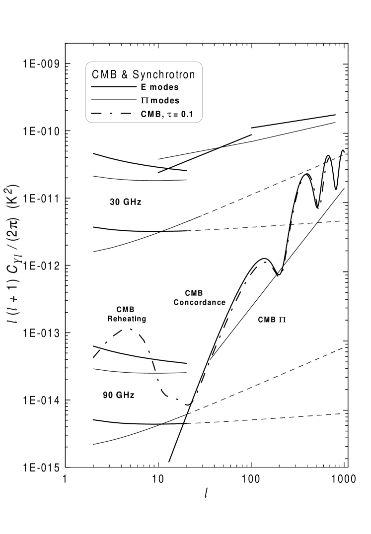
Figure 6: The APS for $E$ mode (thick and dash–dotted lines) and polarized intensity (thin lines). The CMBR concordance model assumes the parameters adopted by Kovac et al. (2002). The thin and dash–dotted CMB lines refer to a model with a reheating optical depth $\tau=0.1$; the polarized intensity curve is a power–law approximation to the output of simulations reported by Tucci et al. (2002). The synchrotron APS are best–fit curves, extrapolated to 30 and 90 GHz from the following maps: The template of Bernardi et al. (2003), $l=2$–20; olation; the intermediate–latitude patch in BS76 (Bruscoli et al. 2002), $l=10$–70; the D97 survey (Tucci et al. 2000), $l=100$–800. For the template of Bernardi et al. (2003) we also give the APS from reduced maps at high Galactic latitudes, with extrapolations to $l=20$–$1000$ represented by dotted lines.

The D97 and D99 surveys showed that Galactic–Plane polarization is not much correlated to total intensity, being often high in the absence of sources in total intensity, and exhibits a foreground component generally supposed to originate locally, i.e. within a few kpc. Local APS have been computed in twelve D97 patches and six D99 patches of size $10^{\circ}\times 10^{\circ}$ (Tucci et al. 2000, 2001) and exhibit moderate slopes $\alpha_{E}$ $\simeq\alpha_{B}\simeq 1.5$, with no systematic differences between high– and low–polarized emission regions. A recent re–analysis of D97 data by another group (Giardino et al. 2002) gives similar results. Out of the Galactic plane, the U99 survey shows larger dispersions in the spectral parameters, due to structures with strong polarized signals (e.g., in the Cygnus and Fan regions) and regions of very low total intensity. Five low–intensity patches with $\alpha_{T}$ $\simeq 0$, which must be dominated in intensity by discrete sources, have been used to infer a rather accurate estimate $C_{Tl}^{\mathrm{(PS)}}\simeq 5\times 10^{-7}$ K² for the sum of all point source populations at 1.4 GHz. Adopting a radio–source polarization degree $\sim 5\%$, the estimate $C_{Pl}^{\mathrm{(PS)}}\sim 1.3\times 10^{-9}$ K² was provided at 1.4 GHz, as well as other estimates at different frequencies with reasonable assumptions on the frequency spectral index (Bruscoli et al. 2002). Such estimates imply that the contribution of point sources should be negligible for all of the polarization APS reported for all of the aforementioned surveys, as confirmed by the fact, that the slopes of polarization APS do not show any flattening towards higher $l$. The impact of Faraday rotation, however, is not clear from the data, and must be investigated looking at different frequencies and angular scales. A multiwavelength study has been performed in the range $l\leq 70$ by Bruscoli et al. (2002) using three large patches of the BS76 survey at various latitudes up to near the Galactic Pole. At such scales no definite trends were found in the spectral slopes for increasing Galactic latitude. A clear flattening of polarization APS, $\alpha_{E,B}\simeq 1$, appears at low frequencies, $\nu\leq 610$ MHz, where Faraday rotation is larger; on the other hand, at 1.4 GHz no significant dependence on Galactic latitude appears, due to the large error bars. Also the APS normalizations are essentially consistent, as shown by Fig. 6. According to the analysis of D97, D99 and BS76 data, the $C_{\Pi l}$ spectra at $\nu\geq 1.4$ GHz may be only slightly steeper than $C_{Pl}$, since the best slope estimate is $\alpha_{\Pi}\simeq 1.6\div 1.7$ and the difference has little statistical significance. The substantial agreement does not prove, however, that the polarization APS at $\nu\geq 1.4$ GHz do reflect the intrinsic properties of synchrotron at all scales.

A more recent analysis of Tucci et al. (2002) in fact shows that this is not the case at 1411 MHz at high resolutions. Rich small–scale structures appear in the ATCA maps (G01) and other polarimetric observations. The sharp–edge patches in the G01 maps of polarization angles are particularly impressive, and strongly suggest that many structures are in fact produced by sharp Faraday–rotation changes in the polarization angle. This has a strong bearing on $C_{El}$ and $C_{Bl}$: The polarization APS computed in a $4^{\circ}\times 4^{\circ}$ box and several smaller patches give $\alpha_{E}$ $\simeq\alpha_{B}\simeq 2.8,$ whereas $\alpha_{\Pi}{}\simeq 1.6$. Such values have been compared to those computed in an overlapping $5^{\circ}\times 5^{\circ}$ box extracted from the D97 survey. Large discrepancies are found for $\alpha_{E}$ and $\alpha_{B},$ $\Delta\alpha\simeq 1$, but not for $\alpha_{\Pi}$. Rescaling the data with a synchrotron spectral index $\beta_{\mathrm{sync}}$ between $-2.5$ and $-3,$ The ATCA $C_{\Pi l}$ spectrum appears to be the natural extension to smaller scales of the corresponding spectrum at $l\leq 800$, since the normalization is also quite consistent. On the other hand, the power excess of $E$ and $B$ modes in the ATCA spectra is nearly one order of magnitude at scales $600\mathrel{\mathchoice{\vbox{\offinterlineskip\halign{\hfil$\displaystyle#$\hfil\cr<\cr\sim\cr}}}{\vbox{\offinterlineskip\halign{\hfil$\textstyle#$\hfil\cr<\cr\sim\cr}}}{\vbox{\offinterlineskip\halign{\hfil$\scriptstyle#$\hfil\cr<\cr\sim\cr}}}{\vbox{\offinterlineskip\halign{\hfil$\scriptscriptstyle#$\hfil\cr<\cr\sim\cr}}}}l\mathrel{\mathchoice{\vbox{\offinterlineskip\halign{\hfil$\displaystyle#$\hfil\cr<\cr\sim\cr}}}{\vbox{\offinterlineskip\halign{\hfil$\textstyle#$\hfil\cr<\cr\sim\cr}}}{\vbox{\offinterlineskip\halign{\hfil$\scriptstyle#$\hfil\cr<\cr\sim\cr}}}{\vbox{\offinterlineskip\halign{\hfil$\scriptscriptstyle#$\hfil\cr<\cr\sim\cr}}}}1000$ and declines at $l$ greater than a few thousand. This excess must be due to Faraday boosts of the polarization angles (Tucci et al. 2002).

2.4.3 A synchrotron template at SPOrt scales

In the light of the aforementioned results, a simple extrapolation of $C_{El}$ and $C_{Bl}$ from $\nu\sim 1$ GHz to higher frequencies is not possible using an $l$–independent spectral index. How can we get rid of Faraday rotation? Giardino et al. (2002) use D97, the total–intensity survey of Haslam et al. (1981) and other radio data to produce a real–space model of polarized synchrotron emission $T$ and $\Pi$; the polarization angle however is just taken as a random quantity, so the final synthetic maps were declared to be a toy model. A more powerful approach has been recently introduced by Bernardi et al. (2003), intended to produce a Faraday–free template of polarized synchrotron. It is based on the following steps: (a) A synchrotron intensity map is built using the 408 MHz total intensity survey of Haslam et al. (1981) and the 1.4 GHz survey of Reich & Reich (1986). Two different frequencies are necessary to clean the maps from free–free emission. (b) The polarized intensity $\Pi$ is modelled, assuming that polarization is produced within a spherical “polarization horizon” and calibrating a normalization factor with comparison with BS76 in the Fan region. (c) A map of polarization angles is built from starlight polarization data, with interpolation from Heiles (2000) catalog and a $90^{\circ}$ rotation. The last step, which assumes an essentially common location for dust selective absorption of starlight and for synchrotron emission, is of crucial importance. Several tests discussed by Bernardi et al. (2003) support the reliability of the template under this respect, and in connection with the polarization horizon modelling for $\Pi$ as well. Due to the Heiles data sampling the template has been provided for an angular scale of $7^{\circ}$. An update of the template, taking advantage of the WMAP intensity maps at 23 GHz, is in preparation. APS computed on Faraday–free templates can be extrapolated to higher frequencies better than those of current surveys. Due to the low resolution, results could be provided by Bernardi et al. (2003) only for $l\leq 20$, where the full–map template gives $\alpha_{P}=1.9\pm 0.2$ and $\alpha_{\Pi}=1.9\pm 0.2$. The substantial agreement with surveys at $2.4$–$2.7$ GHz reinforces both the validity of the template and our previous support to moderate spectral slopes. The high slopes $\alpha_{E,B}\simeq 2.8$ found by ATCA in the SGPS Test Region at 1.4 GHz, on the other hand, must overrate intrinsic synchrotron slopes substantially, being due to the high–$l$ decline of the spectral power excess.

In Fig. 6 we have collected the extrapolations to 30 and 90 GHz of some of the power–law fits to $E$–mode and polarized intensity APS, without attempting to give error bars. Such extrapolations, which at present provide only reasonable guidelines, cover the entire range $l=2$–$1000$ including results from various surveys at $\nu=1.4\div 2.4$ GHz and the aforementioned template. For the template we show the APS derived from both full maps and reduced maps (50%) containing only the lowest–signal pixels; for the latter, the extrapolation to the angular range $l=20\div 1000$ is also provided. Clearly, in view of the differences in the investigated sky regions, coverages and frequencies, one should not expect to find a detailed agreement. However, the curves displayed in Fig. 6 are roughly consistent with each other even for the normalization factor. Only the template APS derived from the reduced maps (with low–signal pixels) have a lower normalization, and suggest that the detection of the secondary–ionization spectral bump should not be hampered by synchrotron at 90 GHz.

3 The SPOrt Experiment

The SPOrt experiment, carried on under the scientific responsibility of an international collaboration of Institutes headed by the IASF–CNR in Bologna, and fully funded by the Italian Space Agency (ASI), was selected by ESA in 1997 to be flown on board the International Space Station (ISS) during the Early Utilization Phase.

The payload, shown in Fig. 7, houses four corrugated feed horns feeding a 22, a 32, and a pair of 90 GHz channels providing direct measurements of the $Q$ and $U$ Stokes parameters. It will be located on the Columbus External Payload Facility of the ISS in 2006, for a mission with a minimum lifetime of 18 months.

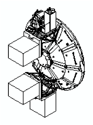
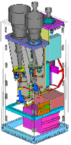
Figure 7: Left: The SPOrt position on the Columbus External Payload Facility, onboard the ISS (courtesy by Alenia Spazio). Right: Expansion of the SPOrt payload.

Table 1: SPOrt main features: $N_{\rm pix}$ is the number of FWHM pixels covered by SPOrt, $\sigma_{1s}$ is the istantaneous sensitivity (1 second), and $\sigma_{\rm pix}$ is the pixel sensitivity for a two–year mission.

${\nu}$	channels	BW	FWHM	Orbit Time	Coverage	$N_{\rm pix}$	${\sigma}_{1s}$	$\sigma_{\rm pix}$
(GHz)	(#)	(∘)		(s)	(%)		(mK s1/2)	($\mu$K)
22	1						0.5	$1.6$
32	1	10%	7	5400	80	660	0.5	$1.6$
90	2						0.57	$1.8$

The SPOrt antennae, looking at the zenit, will cover 80% of the sky thanks to the motion of the Space Station, whose orbit is tilted by $51.6^{\circ}$ with respect to the Celestial equator and is characterized by a period of about 5400 s and a precession of about 70 days. This results in the sky scanning pattern shown in Fig. 8, providing a full coverage of the accessible region every 70 days. In Fig. 8 a map of the time spent over each pixel, of about 7^∘ (HEALPix parameter $Nside=8$), is also shown.

The main features of the SPOrt experiment, summarised in Table 1, have been chosen to allow the accomplishment of SPOrt primary goals, e.g. a tentative detection of CMBR polarization on large angular scales, and the mapping of Galactic synchrotron emission. The former asks for both a nearly all–sky survey and a multifrequency approach to control possible contaminations from Galactic foregrounds; the latter is expected from the channels at 22 and 32 GHz.

The direct and simultaneous measurement of both Stokes parameters $Q$ and $U$ optimizes the observing time efficiency, a remarkable improvement compared to other schemes providing either $Q$ or $U$ and thus reducing it by a factor $2$.

The SPOrt expected sensitivity to CMBR, resulting from the combination of the four channels and taking into account the worsening due to foreground subtraction (Dodelson 1997), is reported in Table 2. In the frame of recent WMAP results on the optical depth of the Universe at the re–ionization epoch, SPOrt promises a solid detection of large scale CMBR polarization.

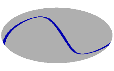
Figure 8: Left: The sky, in Celestial coordinates, as scanned by SPOrt in few orbits. Right: Pixel observing time (seconds) for two years of data taking. The pixel size is about $7^{\circ}$ (HEALPix parameter $Nside=8$).

Table 2: SPOrt sensitivity to CMBR, in thermodynamic temperature, combining the four channels and including Galactic synchrotron subtraction, for a two–year mission.

$\sigma_{1s}$	$\sigma_{\rm pix}$	$\sigma$(Prms)
(mKs1/2)	($\mu$K)	($\mu$K)
0.53	$1.7$	$0.15$

3.1 Instrument Design and Analysis

The main concern in designing an experiment to measure CMBR polarization is the low level of the expected signal (1–10% of the already tiny temperature anisotropies, depending on the scale), requiring specific instrumentation.

The design optimization with respect to systematics generation, long term stability and observing time efficiency is indeed even more critical here than for experiments primarily designed to investigate CMBR temperature anisotropies. This is demonstrated by previous attempts to measure CMBR polarization where the final sensitivity was sizeably worse than that expected from the istantaneous sensitivity of the front–end noise (Keating et al. 2001; Hedman et al. 2002; Kogut et al. 2003).

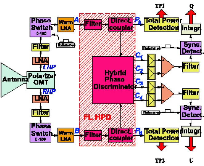
Figure 9: Schematic block diagram of the SPOrt radiometers. Polarizer and OMT extract the two circularly polarized components $LHP$ and $RHP$ collected by the horn. After amplification, the correlation unit (based on a Hybrid Phase Discriminator, see Peverini et al. 2002 for details) provides directly both $Q$ and $U$.

The following main choices were made while designing the polarimeter:

• correlation architecture to improve the stability;

• correlation of the two circularly polarized components $E_{L}$ and $E_{R}$ to directly and simultaneously measure both Q and U from the real and imaginary parts of the correlation, respectively,

  $$\begin{array}[]{rcr}Q\propto\Re(E_{R}E_{L}^{*});&&U\propto\Im(E_{R}E_{L}^{*})\end{array}$$ (20)

  while keeping 100% efficiency;

• detailed analysis of the correlation scheme to identify critical components and set their specifications in order to keep the systematics at a level suitable to measure CMBR polarization;

• custom development of components when state–of–the–art is not compliant with SPOrt requirements;

• on axis simple optics (corrugated feed horns) to minimize the spurious polarization induced by both the $f$ pattern (see Carretti et al. 2001 for its definition) and the CMBR temperature anisotropy on the beam scale.

The equation giving the radiometer sensitivity (Wollack 1995; Wollack et al. 1998)

$$\Delta T_{\rm rms}=\sqrt{{k^{2}\,T_{\rm sys}^{2}\over\Delta\nu\,t}+T_{\rm offset}^{2}\left({\Delta G\over G}\right)^{2}+\Delta T_{\rm offset}^{2}}$$ (21)

can help us find the parameters to be controlled to minimize the systematics. Here $T_{\rm sys}$, $T_{\rm offset}$ and $\Delta T_{\rm offset}$ represent the system temperature, the offset equivalent temperature and its fluctuation, respectively; $G$ is the radiometer gain, $t$ the integration time, $\Delta\nu$ the radiofrequency bandwidth and $k\simeq 1$ a constant depending on the radiometer type.

The first term in Eq. (21) represents the white noise of an ideal and stable radiometer. Its contribution can be reduced by cooling to cryogenic temperature the front–end (first stage of the Low Noise Amplifiers (LNAs), polarizer and the OMT). Unfortunately, passive cooling is not feasible for low orbits because of variations of the Sun illumination. For SPOrt, a mechanical pulse–tube cryocooler was adopted, ensuring high cooling efficiency down to $\sim$80–90 K. The needed temperature stability ($\pm 0.1$ K) is achieved by a closed–loop active control. An active control is also adopted for the warm parts (Horn and back–end), allowing a temperature stability of $\pm 0.2$ K.

The second and the third term of Eq. (21) represent the contributions of gain and offset fluctuations, respectively, generated by instrument instabilities. It is clear that the noise behaviour can be kept close to the ideal (white) case provided the offset is kept under due control.

A scheme of the SPOrt radiometers is sketched in Fig. 9. The Polarizer and the OMT extract the two circularly polarized components $E_{L}$ and $E_{R}$ collected by the dual–polarization feed horn. After amplification, the two components are correlated by the Correlation Unit (CU), consisting of an Hybrid Phase Discriminator (HPD), four diodes and two differential amplifiers. In details, the HPD generates the four outputs:

$$C_{1} \propto E_{L}+E_{R}$$ (22)

$$C_{2} \propto E_{L}-E_{R}$$ (23)

$$C_{3} \propto E_{L}+j\,E_{R}$$ (24)

$$C_{4} \propto E_{L}-j\,E_{R}$$ (25)

which are square–law detected by the four diodes

$$\left|C_{1}\right|^{2} \propto \left|E_{L}\right|^{2}+\left|E_{R}\right|^{2}+2\Re(E_{R}E_{L}^{*})$$ (26)

$$\left|C_{2}\right|^{2} \propto \left|E_{L}\right|^{2}-\left|E_{R}\right|^{2}-2\Re(E_{R}E_{L}^{*})$$ (27)

$$\left|C_{3}\right|^{2} \propto \left|E_{L}\right|^{2}+\left|E_{R}\right|^{2}+2\Im(E_{R}E_{L}^{*})$$ (28)

$$\left|C_{4}\right|^{2} \propto \left|E_{L}\right|^{2}-\left|E_{R}\right|^{2}-2\Im(E_{R}E_{L}^{*}).$$ (29)

The differences performed by the two differential amplifiers provide

$$\begin{array}[]{lllll}\left|C_{1}\right|^{2}-\left|C_{2}\right|^{2}&\propto&\Re(E_{R}E_{L}^{*})&\propto&Q\\ \left|C_{3}\right|^{2}-\left|C_{4}\right|^{2}&\propto&\Im(E_{R}E_{L}^{*})&\propto&U\end{array}$$ (30)

allowing the simultaneous measurement of the two Stokes parameters $Q$ & $U$. A nice feature is that no effort is needed to equalize the mean phase difference between $E_{R}$ and $E_{L}$ when propagating the signal through the instrument, since an error on this difference simply results in a polarization angle rotation, well recoverable in the calibration procedure. Indeed, linear polarization might also be measured by correlating the two linear polarizations $E_{x}$, $E_{y}$. However, this would only provide one linear Stokes parameter ($U$), reducing the experiment efficiency, and would generate a combination of $U$ and $V$ in the output in case of errors in the phase difference. Therefore, great care would be needed in equalizing the path of the two components.

Our analysis to track down critical components for the offset generation pointed out important sources in both the CU and the antenna system (horn, polarizer and OMT).

We found that the CU needs an HPD with high rejection of the unpolarized component, at a level well beyond available instrumentation. A custom device (Tascone et al. 2002; Peverini et al. 2002) providing $>30$ dB rejection was thus developed. In combination with a lock–in system, this makes the CU contribution to the offset negligible, the total rejection being $\simeq 60$ dB.

The contribution to the offset coming from the antenna system is given by (Carretti et al. 2001):

$$T_{\rm offset}=S\!P_{\rm OMT}\left(T_{\rm sky}+T_{\rm noise}^{\rm Ant}\right)+S\!P_{\rm pol}\left(T_{\rm sky}+T_{\rm noise}^{\rm horn}-{T_{\rm ph}^{\rm pol}\over\eta}\right),$$ (31)

where $T_{\rm sky}$ is the signal coming from the sky, $T_{\rm noise}^{\rm horn}$ is the noise generated by the horn alone, $T_{\rm noise}^{\rm Ant}$ is the noise temperature of the whole antenna system, $\eta$ is the efficiency of the feed horn and $T_{\rm ph}^{\rm pol}$ is the physical temperature of the polarizer. The two quantities

$$S\!P_{\rm OMT} = 2\,{\Re(S_{A1}S_{B1}^{*})\over\left|S_{A1}\right|^{2}},$$ (32)

$$S\!P_{\rm pol} = {1\over 2}\left(1-{\left|S_{\perp}\right|^{2}\over\left|S_{\parallel}\right|^{2}}\right),$$ (33)

describe the performances of the OMT and the polarizer, respectively, in terms of offset generation. Uncorrelated signals like noise and sky emission are partially detected as correlated because of the OMT cross–talk ($S_{A1}$ and $S_{B1}$ representing the transmission and cross–talk coefficients of the OMT, respectively) and the polarizer attenuation difference ($S_{\parallel}$ and $S_{\perp}$ giving the transmissions of the two polarization states).

To set specification requirements for our OMT and polarizer we considered the radiometer knee frequency, $f_{\rm knee}$. This parameter provides the time scale at which the low frequency component of the noise, also known as 1/$f$, prevails on the white one, and is therefore suitable to quantify radiometer instabilities.

Figure 10: Magnitude of both the isolation between the two rectangular ports and the cross–talk between the two polarization states for the 32 GHz OMT of SPOrt. The vertical dotted lines define the 10% band.

As is known, destriping techniques can remove most of the effects of 1/$f$ noise provided the radiometer knee frequency is lower than the signal modulation frequency (see Sect. 3.3) that, for SPOrt, corresponds to the orbit frequency $f_{\rm o}=0.18$ mHz.

Currently available InP LNA have rather high knee frequencies ($f_{\rm knee}^{\rm lna}\sim$ 100–1000 Hz). However, the knee frequency of a correlation receiver is related to that of its amplifiers by the formula:

$$f_{\rm knee}=\left({T_{\rm offset}\over T_{\rm sys}}\right)^{2/\alpha}f_{\rm knee}^{\rm lna}$$ (34)

where $T_{\rm offset}$ is the radiometric offset, $T_{\rm sys}$ the system temperature and $\alpha\sim 1$ (Wollack 1995) is the power–law index of the LNA’s $1/f$ noise behaviour.

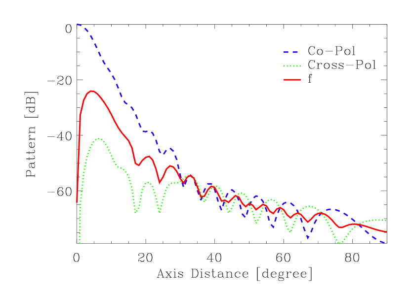
Figure 11: Co–polar, cross–polar and $f$ patterns, with respect to the axis distance $\theta$, for the 90 GHz feed horns of SPOrt . The spurious polarization coming from the horn is generated by the anisotropy distribution $\Delta T(\theta\phi)$ in combination with the $f$ pattern (see text).

To match the condition for a successful destriping ($f_{\rm knee}<f_{\rm o}$, with $f_{\rm knee}=0.1f_{\rm o}=0.018$ mHz as a goal), SPOrt requirements on the OMT cross–talk and the difference between the attenuations of the two polarization states were quantified in $-60$ dB and $-30$ dB, respectively. This guarantees an offset value as low as $T_{\rm offset}\sim$ 50 mK which, combined with a $T_{\rm sys}\sim$ 100 K, translates into the knee frequency

$$f_{\rm knee}\sim 2.5\times 10^{-7}f_{\rm knee}^{\rm lna}$$ (35)

fully satisfying the requirements for an efficient destriping.

Commercially available state–of–the–art OMTs have isolation values not better than $-40$ dB, which forced us to develop new hardware. Fig. 10 shows the extremely good results already obtained for the 32 GHz channel: the cross–talk is as low as $-65$ dB, with an isolation of about 70 dB.

Besides the offset generation, a further worrysome source of systematic errors is the spurious polarization generated by the optics (Carretti et al. 2001). This is due to the anisotropy distribution of the unpolarized radiation, modulated by the $f$ pattern:

$$\Delta T^{\rm horn} = {1\over\Omega_{A}}\int_{0}^{\pi}\sin\theta\,d\theta\int_{0}^{\pi/2}\left[\Delta T_{b}(\theta,\phi)\right.$$ (36)

$$- \Delta T_{b}(\theta,\phi+\pi/2)+\Delta T_{b}(\theta,\phi+\pi)$$

$$- \left.\Delta T_{b}(\theta,\phi+3/2\pi)\right]\,f(\theta,\phi)\,d\phi\,,$$

$$f(\theta,\phi) = -P(\theta,\phi)\chi^{*}(\theta,\phi+\pi/2)$$ (37)

$$+ \chi(\theta,\phi)P^{*}(\theta,\phi+\pi/2)\,,$$

where $P$ and $\chi$ are the co–polar and cross–polar patterns, normalized to the P maximum, respectively, and $\Omega_{A}$ is the antenna beam. The $f$ pattern consists of a 4–lobe structure, with lobe size close to the FWHM of the instrument. A worst–case analysis of the contamination gives

$$\Delta T^{\rm horn}=S\!P_{\rm horn}\,\,\Delta T_{\rm rms}({\rm FWHM})\,,$$ (38)

with

$$S\!P_{\rm horn}=2\,{1\over\Omega_{A}}\int_{0}^{\pi}\sin\theta\,d\theta\int_{0}^{\pi/2}\,d\phi\,f(\theta,\phi)$$ (39)

and $\Delta T_{\rm rms}({\rm FWHM})$ the rms temperature anisotropy on FWHM scale. As shown in Fig. 11, in case of the SPOrt feed horns the contribution of the $f$ pattern is $S\!P_{\rm horn}\sim-24$ dB and the rms contamination due to the 30 $\mu$K–CMBR anisotropy is thus lower than 0.2 $\mu$K.

3.2 Calibration procedure

The accuracy needed for measuring CMBR polarization requires good methods for calibrating the response of the instrument to small polarized signals. Furthermore, in the absence of well–characterized astrophysical sources, specialized techniques are needed to inject calibration markers. In fact, standard marker injectors are not suitable for calibrating tensorial quantities as the ($Q$, $U$) pair measured by SPOrt. A new concept calibrator, valid for any radio–polarimeter and based on the insertion of three signals at different position angles, has thus been developed (Baralis et al. 2002).

To focus the problem it is convenient to represent the entire radiometer in terms of a system with two input and output signals. The two inputs $A$ and $B$ are high frequency signals in the circular polarization base ($E_{L}$ and $E_{R}$), whereas the two outputs $Q_{m}$ and $U_{m}$ are the low frequency signals corresponding to the Stokes parameters directly measured by the radiometer. According to this model, the output of the radiometer can be described by the following matrix expression:

$$\left[\matrix{Q_{m}\cr U_{m}}\right]=\left[\matrix{H_{qq}&H_{qu}\cr H_{uq}& H_{uu}}\right]\left[\matrix{Q\cr U}\right]+\left[\matrix{T_{qa}&T_{qb}\cr T_{ua}& T_{ub}}\right]\left[\matrix{|A|^{2}\cr|B|^{2}}\right]$$ (40)

where $Q$ and $U$ are the input Stokes parameters. The matrices $\underline{\underline{H}}$ and $\underline{\underline{T}}$ in Eq. (40) are generic, but real, since they deal with quadratic quantities. Moreover, they transform polarization circles in the $QU$–plane into rotated and translated ellipses. Under the reasonable assumption that the intensities of the total signals $A$ and $B$ are equal ($|A|^{2}=|B|^{2}\propto P$), Eq. (40) can be rewritten as $\underline{Y}=\underline{\underline{H}}\,\underline{X}+\underline{C}\,P$, where $\underline{C}$ is a two–element column vector. The calibration procedure, i.e. the evaluation of the matrices $\underline{\underline{H}}$ and the vector $\underline{C}$, can be accomplished by directly measuring the quantities $Q_{m}$ and $U_{m}$ in presence of predefined signals (markers). In fact, by injecting at different times three markers with known polarization angles $\theta_{i}$, each corresponding to a linearly polarized field, and by detecting the corresponding output variations, one ends up with a matrix equation to be solved for the matrix $\underline{\underline{H}}$:

$$\underline{\underline{H}}\left[\matrix{\frac{\Delta\underline{X}_{3}}{\Delta P_{3}}-\frac{\Delta\underline{X}_{1}}{\Delta P_{1}} \frac{\Delta\underline{X}_{2}}{\Delta P_{2}}-\frac{\Delta\underline{X}_{1}}{\Delta P_{1}}}\right]=\left[\matrix{\frac{\Delta\underline{Y}_{3}}{\Delta P_{3}}-\frac{\Delta\underline{Y}_{1}}{\Delta P_{1}}\;,& \frac{\Delta\underline{Y}_{2}}{\Delta P_{2}}-\frac{\Delta\underline{Y}_{1}}{\Delta P_{1}}}\right]$$ (41)

where $\Delta\underline{X}_{i}$, $\Delta\underline{Y}_{i}$ and $\Delta P_{i}$ are the variations of the input and output Stokes parameters and of the total power, respectively. To obtain a well–conditioned matrix the markers should correspond to signals with a relative rotation of either 45^∘ or 60^∘.

3.2.1 Marker injector

The calibration procedure described in the previous section requires the injection of different markers in the radiometer, just behind the antenna. Unfortunately, this procedure must be carried out in operative conditions, e.g. in presence of both polarized and unpolarized radiation. Therefore, the marker injector must degrade the relevant signals as little as possible. In particular, this device has to exhibit a high return loss and prevent depolarization of the incoming signals.

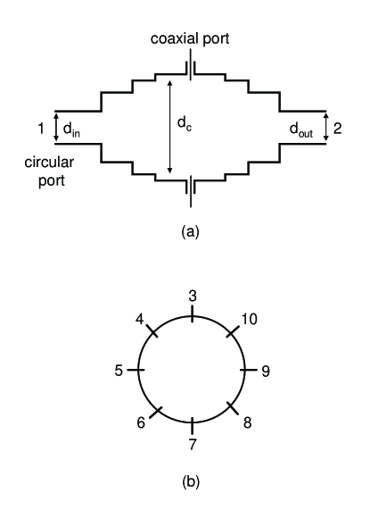
Figure 12: Scheme of the marker injector. a) Longitudinal cut. b) Cross–section of the central block.

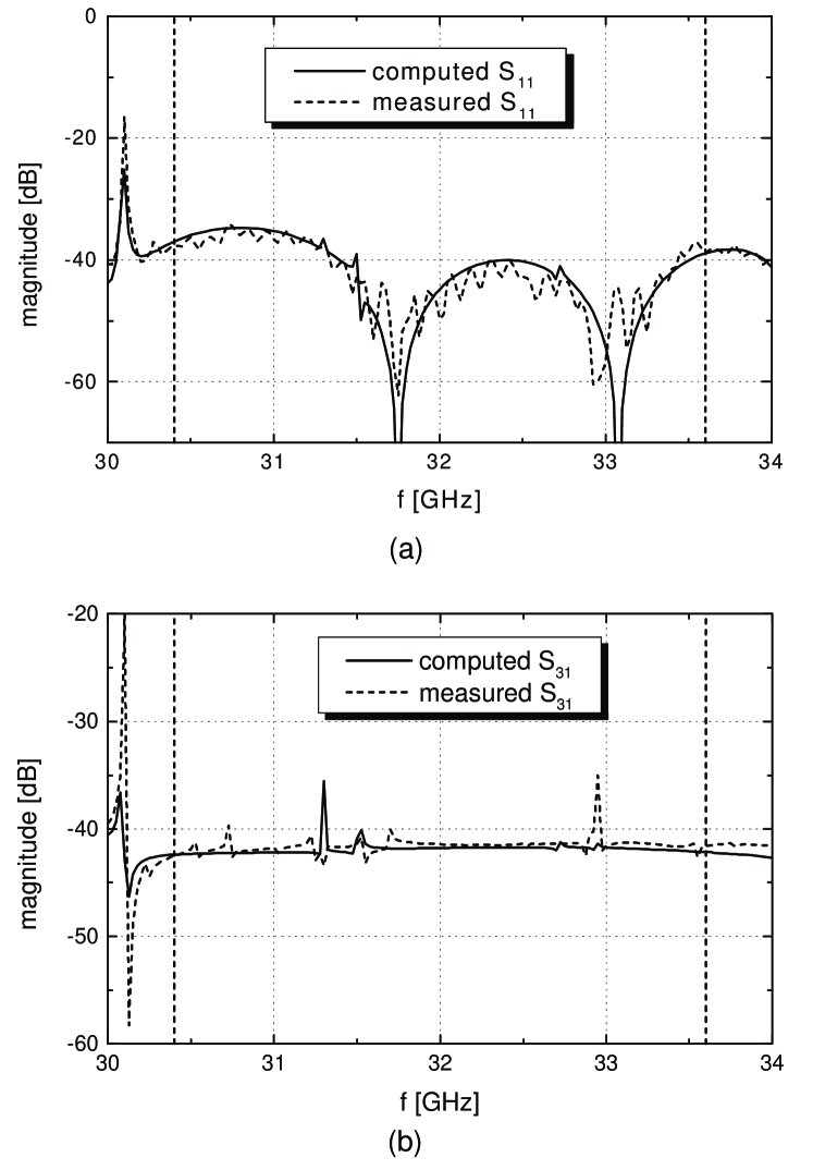
Figure 13: Measured an computed scattering parameters of the Ka–band marker injector. Top: Reflection coefficient. Bottom: Coaxial/circular coupling factor. Vertical dashed lines define the SPOrt band.

The design of the Ka–band prototype is depicted in Fig. 12, and consists of three blocks (Peverini et al. 2002b). The central block is formed by an enlarged circular waveguide in which eight K–connectors are inserted. Although only three markers have to be injected inside the circular waveguide, all the eight connectors are necessary to preserve the azimuthal symmetry of the structure and, hence, to avoid depolarization of the incoming signals. The coupling level between coaxial and circular ports can be controlled by adjusting the penetration length of the internal wire of the K–connectors. The two lateral blocks provide a matching structure between the input/ouput circular waveguides and the enlarged central waveguide. The matching section is formed by a cascade of several circular steps. The device was analyzed by the Generalized Scattering Matrix approach (Itoh 1989) and designed by evolution–strategy methods. All the components were manufactured by highly precise electrical–discharge techniques.

In Fig. 13 the measured and simulated reflection coefficient $S_{11}$ at the circular port for the fundamental TE₁₁ mode and the coupling $S_{31}$ between circular and coaxial ports are reported. The measured coaxial/circular coupling factor is $\approx-42\,\rm dB$ in all the band of interest ($30.4\div 33.6\,\rm GHz$) and the fundamental mode at the circular port exhibits a reflection coefficient better than $-35\,\rm dB$ in the same band. The measured in–band insertion loss is about 0.02 dB, which can be correctly predicted by using an equivalent surface resistance of $10\,\rm\mu\Omega cm$.

3.3 Destriping and Map Making

Low frequency noise induces correlations among successive samples of the measured signal and leads to typical striping effects when producing sky maps.

However, when data are taken from spinning spacecrafts, most of the low frequency noise can be removed by software, provided the radiometer knee frequency is lower than the satellite spin frequency (Janssen et al. 1996). As detailed in Sect. 2.1.1, the low frequency noise of the SPOrt radiometers is expected to have a $1/f$–like spectrum dominated by transistor gain fluctuations. The present state of the instrument already guarantees a knee frequency $f_{\rm knee}$ lower than the ISS orbit frequency $f_{o}$.

Various destriping algorithms have been proposed in recent years to clean CMBR anisotropy data (e.g. Delabrouille 1998; Maino et al. 1999), together with a first algorithm specifically designed for the polarization case (Revenu et al. 2000). They are generally based on $\chi^{2}$ minimizations and involve large matrix inversions.

A different technique has been implemented for SPOrt (Sbarra et al. 2003), consisting of a simple but effective iterative algorithm relying upon minimal assumptions: the radiometer must be stable during the signal modulation period (the time needed to complete one orbit in case of SPOrt), so that the instrumental offset can be assumed to be constant over the same period, and there must be enough overlap between different orbits. In such a situation the noise can be split into two parts: for time scales shorter than the orbit period it is essentially white, whereas for longer timescales the $1/f$ component can be modelled as a different constant offset for each orbit. A simple iterative procedure can then be applied to remove these offsets from the Time Ordered Data (TOD) before map–making. No assumptions need to be made about the statistical properties of the noise. The map–making itself consists of a simple average of the measurements corresponding to the same pixel, which is the optimal method once only white noise is left (Tegmark 1997).

Although the algorithm has been studied to destripe $Q$ and $U$ data, it can be easily simplified to deal with scalar quantities. The average of the measured signal is lost in the latter case. However, for maps of polarization data like $Q$ and $U$, the average signal can still be kept provided the polarimeter reference frame rotates about the standard reference frame (polar basis, see Berkhuijsen 1975) while running along each orbit, as in case of SPOrt. This is a nice feature, especially when measuring foreground contributions.

The good performances of the technique are made evident in Fig. 14 where we show a simulated noise map (both $1/f$ and white) before and after destriping.

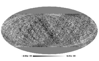
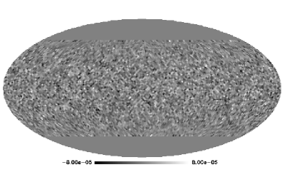
Figure 14: Noise simulated maps before (top) and after (bottom) destriping, for the case $f_{\rm knee}=1.8\cdot 10^{4}$, in Kelvin. The HEALPix parameter $Nside$ is 32 (courtesy of A&A).

Table 3: Excess rms noise due to low–frequency contributions, with respect to the white noise level, for pixels of $\simeq 7^{\circ}$.

$f_{\rm knee}$ (Hz)	Before Destriping	After Destriping
$1.8\times 10^{-4}$	310%	6%
$1.8\times 10^{-5}$	35%	$<1$%

Figure 15: Average and 1$\sigma$ band of correlation functions $C^{Q}(\theta)$ measured from 500 noise maps, before and after destriping, for two values of the knee frequency $f_{\rm knee}$. Before destriping the $y$ scale is not the same for the two $f_{\rm knee}$ values. Each simulation corresponds to about one year of SPOrt realistic data taking. The case of purely white noise is shown for comparison (courtesy of A&A).

Figure 16: Increment, due to the presence of residual correlated noise, in the rms of measured noise power spectra, after destriping, as a function of the multipole, in percentage of the rms of purely white–noise power spectra (courtesy of A&A).

One possible way to quantify the quality of the destriping is measuring the fractional excess pixel noise with respect to the case of purely white noise. Results are shown in Table 3 for two different values of the knee frequency, corresponding to the SPOrt goal knee frequency, $f_{\rm knee}=1.8\times 10^{-5}$ Hz, and the SPOrt orbit frequency, $f_{\rm o}=1.8\times 10^{-4}$ Hz, the latter representing a conservative case.

Another way to quantify the residual correlated noise is measuring and inspecting the two–point correlation functions C${}^{Q}(\theta)=\langle Q(1)Q(2)\rangle$ and C${}^{U}(\theta)=\langle U(1)U(2)\rangle$ (see Sect. 2.1.1) of simulated $Q$ and $U$ noise maps. Averages and 1$\sigma$ bands of 500 correlation functions C${}^{Q}(\theta)$ measured from maps containing both white and $1/f$ noise, before and after destriping, are compared to the purely white noise case in Fig. 15 for the same knee frequencies as in the previous test. As expected, the correlated noise is strongly reduced by the destriping procedure, the residuals falling within the statistical error of the white noise case for $f_{\rm knee}=f_{\rm knee}^{\rm goal}$.

The polarization power spectra $C_{El}$ and $C_{Bl}$ can be obtained from the measured correlation functions by inverting Eqs. (2.1.1) (Kamionkowski et al. 1997b; Zaldarriaga 1998; Ng & Liu 1999). If the correlation functions are measured directly on $Q$ and $U$ maps via $O(N_{\rm pix}^{2})$ operations ($N_{\rm pix}$ being the number of pixels in the measured map), this method (Sbarra et al. 2003) has the advantage of avoiding edge problems (Chon et al. 2003) arising when using fast spherical transforms.

The region of low multipoles is the most sensitive to low frequency residuals, some contributions being always found here even after the application of other destriping techniques (Maino et al. 1999). Even though residual noise correlations can be modelled and subtracted from the measured $C^{Q,U}(\theta)$ functions before integration, their presence translates into an increment of the rms of the measured power spectra. A rough estimate for the case of SPOrt is shown in Fig. 16.

4 Astrophysics and Cosmology with SPOrt

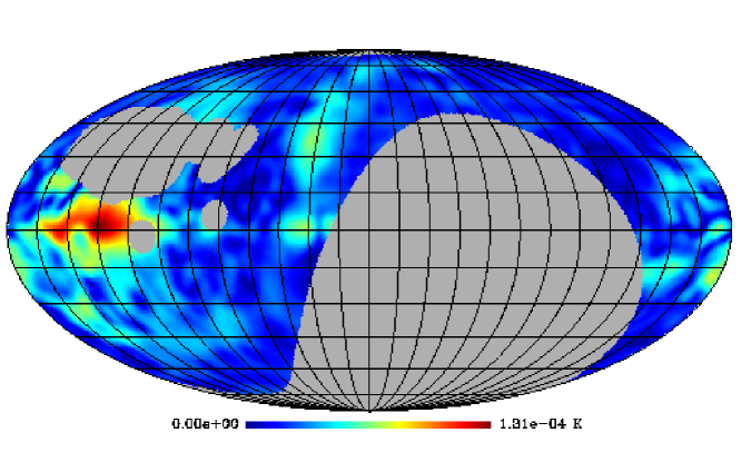
Figure 17: Synchrotron template at 22 GHz (see Sect. 2.4.3), featuring a $P_{\rm rms}=17\mu$K.

A first goal that SPOrt will achieve is a deeper knowledge of the polarization of the Galactic signal, in the microwave band. In particular, according to the synchrotron template described in Sect. 2.4.3, which we believe to be not too far away from reality, SPOrt should be able to produce polarized Galaxy maps at both 22 and 30 GHz. In fact, as shown in Fig. 17, the synchrotron polarized emission, as seen by the $7^{\circ}$–FWHM SPOrt optics at 22 GHz, is expected to have a peak of about $100\,~{}\mu$K, two orders of magnitude larger than the experimental pixel sensitivity in the same channel ($\sigma_{\rm pix}=1.6~{}\mu$K); furthermore, the average of the polarized signal is $P_{\rm rms}=17~{}\mu$K. Assuming a power–low dependence on the frequency with index $\beta_{\rm synch}=-3$, the polarized intensity at 30 GHz is then expected to be just a factor 2–3 lower than at 22 GHz, so that SPOrt is likely to provide a Galaxy map at this frequency as well.

The SPOrt pixel sensitivity quoted in Table 2 does not allow the building of CMBR polarization maps. However, a CMBR band power spectrum as that shown in Fig. 18 is expected to be provided if the recent WMAP results are confirmed. 1–$\sigma$ error bands are calculated following the recipe provided by Tegmark (1997). The plot also suggests that a non–null (at 95%C.L.) measurement of the mean polarized signal $P_{rms}$ might be provided, already for $\tau\simeq 0.1$, by full–sky statistical analyses like the Maximum Likelihood flat–spectrum analysis developed by Zaldarriaga (1998).

Figure 18: $1-\sigma$ error bands, as expected from SPOrt measurement of the $C_{El}$ power spectrum, including cosmic variance, considering the sensitivity quoted in Table 2 and $\tau=0.17$, as recently found by WMAP. APS corresponding to $\tau=0.1$ and $\tau=0.05$ are shown for comparison.

In addition to measuring two low–multipole bands of the $C^{E}_{l}$ power spectrum, combining SPOrt polarization data with WMAP temperature data will provide a measurement of the $C^{TE}_{l}$ power spectrum where errors on $T$ will be completely decorrelated from those on $Q$,$U$.

4.1 Measuring the reionization history of the Universe

In this subsection we briefly describe our procedure to work out cosmological parameters from SPOrt data, stressing, in particular, our expected capacity to inspect the actual value of the cosmic opacity $\tau$ to CMBR photons. $Q$ and $U$ maps are assumed to be free from foreground contamination, the sensitivity worsening coming from this separation, estimated with the procedure suggested by Dodelson (1997), being already included in the quoted pixel sensitivity (see Table 2 in Sect. 3).

In particular, we shall recall and extend previous results by Colombo & Bonometto (2003), showing how measurements on $\tau$ and $n_{s}$ (primeval spectral index) are far less degenerate when polarization data are exploited, at variance from what happens if anisotropy data only are used.

SPOrt large beamwidth allows us to bin data in a fairly low number of pixels ($\sim 2400$ for a HEALPix parameter $Nside=16$, yielding a mean angular distance $\sim 3.5^{\circ}$ between pixel centres); therefore, working in the angular (pixel) space is not numerically expensive; moreover this choice eases the combination of data from experiments with different sky coverages and detector specifications, as we expect to have for anisotropy and polarization: anisotropy data specify $T$ on $N_{T}$ pixels and polarization data specify $Q$ and $U$ on $N_{P}$ pixels. We order data into a $(N_{T}+2N_{P})$–component vector ${\bf x}\equiv\{T(i=1,...,N_{T}),Q(i=1,....,N_{P}),U(i=1,....,N_{P})\}$.

We build artificial data sets, binned according to HEALPix, by using CMBFAST. Data are realizations of a given cosmological model $\mathcal{M}$ and, in each data–map, a white noise map in included. Therefore, the correlation matrix $\langle{\bf x^{T}}_{i}{\bf x}_{j}\rangle\equiv{\bf C}_{ij}={\bf S}_{ij}+{\bf N}_{ij}$ (brackets mean ensemble average) is the sum of a signal term $\bf S$_ij, which depends on cosmology and can be evaluated using the relations given in Sec. 2.1.1, and a term ${\bf N}_{ij}$, which accounts for the detector noise. We assume no correlation among noise in different modes and pixels, so that $\bf N$_ij is diagonal and has distinct values $\sigma_{T}^{2}$ and $\sigma_{P}^{2}$, in $N_{T}$ and $2N_{P}$ pixels, respectively.

Making use of the matrix ${\bf C}_{ij}$, the likelihood of a model $\mathcal{M}^{\prime}$ given the synthetic data x reads:

$${\mathcal{L}}({\mathcal{M}^{\prime}}|{\bf x})=[(2\pi)^{N_{T}+2N_{P}}\det{\bf C^{\prime}}]^{-1/2}\exp[-{\bf x}^{\rm T}{\bf C^{\prime}}^{-1}{\bf x}/2]~{}.$$ (42)

Confidence regions in parameter space are found by a likelihood ratio criterion. This procedure is applied to extract cosmological parameters, by inspecting sets of models ${\mathcal{M}}^{\prime}$ against real data.

Confidence regions in the $n_{s}$–$\tau$ plane are obtained while keeping the other parameters at the fixed values: $\Omega_{m}=0.35$, $\Omega_{\Lambda}=0.65$, $\Omega_{b}=0.05$, $h=0.65$, and assuming no tensor modes. Disentangling $\tau$ and $n_{s}$ measurements is a typical degeneracy removal allowed by polarization data.

All models considered here reionize at the nearest possible redshift, where baryonic materials undergo a (nearly) sharp transition from $x_{e}\simeq 0$ to $x_{e}\simeq 1$. In Sec. 2.3 we outlined that this simple reionization history, not only is not unique, but could also be rather unlikely, if the highest values of $\tau$ found by the first–year WMAP release are confirmed. In that section, however, we also showed that detecting details in the reionization history, at our expected level of sensitivity, is hard (although some indication is possible), while the polarization signal is grossly affected by the overall $\tau$ value. Hence, considering just the case of sharp reionization does not limit the significance of our conclusions. We show results obtained if the model $\mathcal{M}$ has spectral index $n_{s}=1$; but significant quantitative shifts occur only for true $n_{s}$ values unexpectedly different from unity.

The SPOrt sensitivity quoted in Table2 corresponds to a pixel noise

$$~{}~{}~{}~{}~{}~{}~{}~{}~{}~{}~{}~{}~{}~{}~{}~{}\sigma_{P}=3.3\,\sqrt{{2\,{\rm yr}\over\Delta t}{1\over E_{0}}}~{}~{}\mu{\rm K}$$ (43)

for an $Nside=16$ pixilation; here $\Delta t$ and $E_{0}$ are the flight duration and the detection efficiency, respectively. Previous analysis carried out by Colombo & Bonometto (2003) explored the cases $\sigma_{P}=4\,\mu$K, and $\sigma_{P}=2\,\mu$K. In this paper we report results for $\sigma_{P}=3\,\mu$K as well, this value being closer to the SPOrt expected sensitivity. For anisotropy data, assumed to originate from an independent experiment, we take $\sigma_{T}=2\,\mu$K. A similar noise is typical of WMAP anisotropy data, once rescaled to our apertures. Cosmic and noise variances are taken into account by performing 1000 independent realizations of the model $\mathcal{M}$.

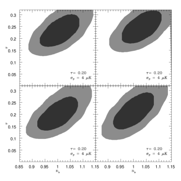
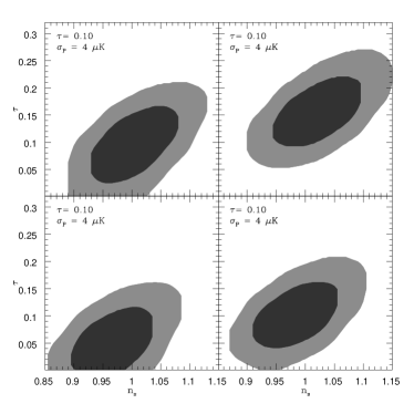
Figure 19: Likelihood contours from the analysis of both polarization ($Q$ and $U$) and anisotropy data, with $\sigma_{P}=4\,\mu$K and $\sigma_{T}=2\,\mu$K, for $\tau=0.20$ (left) and $\tau=0.10$ (right). We assumed a flat model with DE due to cosmological constant, $\Omega_{m}=0.3$, $h=0.65$, $\Omega_{b}h^{2}=0.22,n_{s}=1$. Four independent realizations of the model are shown (see text). More or less heavily shaded areas indicate 1 or 2–$\sigma$ confidence regions, on the $n_{s}$–$\tau$ plane.

In Figs. 19–20 we show joint confidence regions obtained in four realizations, chosen at random, for three different values of $\tau$ in the model $\mathcal{M}$, with $\sigma_{P}=4\,\mu$K. as well as a realization with $\sigma_{P}=2\,\mu$K.

A plot similar to Figs. 19–20 is shown by Spergel et al. (2003), reporting WMAP results. A direct comparison shows that we expect to constrain $\tau$ better than the 1–year WMAP release, already with $\sigma_{P}=4\,\mu$K.

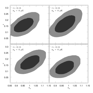
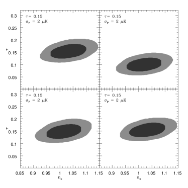
Figure 20: As in Fig. 19, with $\tau=15$ and either $\sigma_{P}=4\,\mu$K (left) or $\sigma_{P}=2\,\mu$K (right).

Let us also stress that, on very large angular scales, information on the optical depth is carried almost exclusively by the polarization (and cross–correlation) APS. This can be seen by comparing the likelihood contours in Fig. 20, where the noise on $T$ data is the same.

In Fig 21 we show the likelihood contours, averaged on cosmic and noise variances, for $\sigma_{P}=3\,\mu$K. Average results are often used to describe the expected performance of an experiment. However, when the likelihood distribution is not expected to approach a Gaussian behaviour, a more detailed analysis of how cosmic and noise variance can affect data is in order.

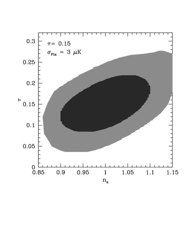
Figure 21: Average likelihood distribution, from the analysis of both polarization ($Q$ and $U$) and anisotropy data, with $\sigma_{P}=3\,\mu$K and $\sigma_{T}=2\,\mu$K. The underlying model is the same as in Fig 19. 1 or 2–$\sigma$ confidence regions, in the $n_{s}$–$\tau$ plane, are shaded as in previous figures.

Figure 22: Fractions of realizations where a lower limit on $\tau$ is found, at different confidence levels, assuming $\sigma_{T}=2\,\mu$K and three different values for $\sigma_{P}$.

Accordingly, Fig. 22 shows in which fraction of realizations various $\tau$ limitations can be achieved. Already for $\sigma_{P}=4\,\mu$K, minimum and maximum values of $\tau$ are detectable in 90$\,\%$ of realizations, at 2–$\,\sigma$ level, provided that the real $\tau\mathrel{\mathchoice{\vbox{\offinterlineskip\halign{\hfil$\displaystyle#$\hfil\cr>\cr\sim\cr}}}{\vbox{\offinterlineskip\halign{\hfil$\textstyle#$\hfil\cr>\cr\sim\cr}}}{\vbox{\offinterlineskip\halign{\hfil$\scriptstyle#$\hfil\cr>\cr\sim\cr}}}{\vbox{\offinterlineskip\halign{\hfil$\scriptscriptstyle#$\hfil\cr>\cr\sim\cr}}}}0.18$. If $\tau\simeq 0.14$, such percentage reduces to $\sim 60\,\%$. These figures should not be confused with those obtainable from the average likelihood. In the latter case, still for $\sigma_{P}=4\,\mu$K and at the 2–$\sigma$ level, the minimum $\tau$ value should be distinguishable from zero if the real $\tau$ is just above 0.10. In this very case, there is also a 20$\ \%$ of a–priori probability that a minimum value of $\tau$ is fixed at the 3–$\sigma$ level.

For the case $\sigma_{P}=3\,\mu$K, minimum and maximum $\tau$ values can be detected, in 90$\,\%$ of realizations, at 2(3)–$\,\sigma$ C.L., provided that the real $\tau>\sim 0.12(0.14)$. Such percentage reduces to $\sim 60\,\%$ only if the real $\tau$ is below 0.07 (0.085). Then, if we refer to the average likelihood, $\tau$ should be lower than 0.06 not to be distinguished from zero.

It is however worth pointing out that, even if $\tau$ was as low as 0.03, a value smaller than the lower WMAP limit, we should still have a $\sim 30\,\%(20\,\%)$ probability to distinguish it from zero at 2(3)–$\sigma$ C.L. Most of these estimates can be deduced from Fig. 22, in which we also point out the case $\tau=0.17$, as from WMAP peak probability.

Let us remind that an improvement in $\tau$ determination is certainly welcome, as widely discussed in Sec. 2. Large $\tau$ values were the main finding of the first–year WMAP release and the physical implications of such $\tau$’s concern the evolution of the Universe at the eve of object formation. Such results arise from the TE correlation at small $l$. Testing such correlation on data coming from instruments measuring $T$ and Stokes parameters separately is, in our opinion, extremely important and urgent.

5 Conclusions

The recent results of the NASA–WMAP satellite put particular emphasis on the importance of CMBR–polarization investigations on large scales, able to either confirm or revise the estimate $\tau=0.17$ obtained from the $C_{TEl}$ spectrum of the WMAP first–year data. Such an unexpectedly high value of $\tau$ suggests fascinating scenarios, some of them discussed in Sect. 2.3, like a double reionization. However, due to systematics still to be fully understood, WMAP did not produce any polarization map yet. Thus, after their first results, there are more and more reasons for investigating large–scale properties of CMBR polarization, independently from the anisotropy.

Previous attempts to measure the CMBR polarization had already demonstrated that the istantaneous sensitivity of the instruments, which essentially depends on the front–end noise, does not always reflect in the final sensitivity. This was due to the presence of systematics cancelling out the advantages of long integration times. Such systematics have been widely treated for anisotropy experiments, but not so deeply for polarization experiments that led to positive detections much more recently.

The SPOrt experiment represents the first attempt to measure the $Q$ and $U$ Stokes parameters of the microwave sky on large angular scales as direct outputs of the instrument. No off–line process is needed to extract the primary information, e.g. the linear polarization in each pixel as defined by the $7^{\circ}$ FWHM of each SPOrt antenna. The SPOrt radiometers have been designed to minimize every source of systematics (in polarization) following an original analytical approach that could lead the way to next generation instruments aiming at B–mode investigations of CMBR. A quite new philosophy, in fact, has been adopted beginning from the identification of the most critical parts of the instrument, passing through their requirement definition and ending up with custom realization of components that actually represent a new state–of–the–art.

Following this idea several new devices have been realized, as for example the onboard calibrator, based on a complex of marker injectors, that allows a full monitoring of the instrument response. The analog correlation is performed by a custom passive microwave device, namely the Hybrid Phase Discriminator and, similarly, other critical components of the SPOrt radiometers have been realized reaching performances often two–three orders of magnitude better than equivalent off–the–shelf components.

As far as data–reduction and analysis are concerned, a new destriping technique has been studied to minimize the correlated noise due to residual systematics and typically affecting the low order multipoles, where most of the cosmological information resides. As a consequence, the SPOrt capability to measure large scale CMBR polarization shall be similar to that of WMAP. Although it is not as high as that planned by PLANCK, SPOrt will make use of true polarimeters.

In parallel to the efforts on both the analysis and the technological development, a relevant activity has also started for understanding and modelling the expected major source of polarized foreground, e.g. the Galactic synchrotron radiation. Existing data sets on Galactic polarized emission, unfortunately limited to regions around the galactic plane and frequencies below 2.7 GHz, have been studied in their spectral and angular properties. Since it was recognized that any simple extrapolation from few GHz to much higher frequencies would fail, the strategy was to build a template estimating the synchrotron polarized emission free from Faraday rotation. The result is a Faraday–free template whose computed APS can be extrapolated up to 90 GHz, at least for multipoles $l<20$.

In summary, SPOrt can be expected to provide a direct measurement of $\tau$, discriminating it from zero at the 2–$\sigma$ level, if the real $\tau>\sim 0.06$. This assumes an excellent performance of observational apparati, leading to a pixel sensitivity $\sigma_{P}=3\,\mu$K for a HEALPix–like pixilation with $Nside=16$. Actual results, of course, are subject to cosmic and noise variances. If we consider that in more detail, minimum and maximum $\tau$ values can be detected, in 60$\,\%$ (90$\,\%$) of realizations, at 2$\,\sigma$ level, if the real $\tau>\sim 0.075$ (0.12). Finally, if $\tau\simeq 0.17$, according to WMAP peak probability, not only considering the average likelihood, but also in 83$\,\%$ of realizations, the detected value will be distinguishable from zero at the 3–$\sigma$ level.

Furthermore, at the 1–$\sigma$ level, some separate information on the reionization redshift $z_{ri}$ and ionization rate $x_{e}$ may be obtainable (see Fig. 3). In the same way, we can hope to put some constraints on the nature of Dark Energy, thanks to the effects on CMBR of different ISW patterns. The SPOrt capability to obtain separate information on cosmic reionization histories and DE nature, is however to be explored in more detail. It should never be forgotten that the SPOrt outputs will be completely free of any possible bias due to instrumental polarization–anisotropy correlation.

Besides testing reionization and discriminating between different values of the Universe optical depth, which is its most appealing goal, SPOrt will provide almost full sky polarization maps of the Galaxy at 22 and 32 GHz. Last but not least, SPOrt will allow testing of new technologies presently beyond the state of the art, thus opening a real window upon more challenging scientific and civil space applications.

References

- [1] Baralis, M., Peverini, O.A., Tascone, R., et al. 2002, in Astrophysical Polarized Backgrounds, Bologna, Italy, October 9–12 2001, ed. S. Cecchini, S. Cortiglioni, R. Sault & C. Sbarra, AIP Conf. Proc. 609, 257
- [2] Becker, R. H., Fan, X., White, R. L., et al. 2001, AJ, 122, 2850
- [3] Bennett, C. L., et al. 1996,ApJ, 464, L1
- [4] Bennett, C., Hill, R.S., Hinshaw, G., et al. 2003, ApJS, 148, 97
- [5] Berkhuijsen, E. M. 1975, A&A, 40, 311
- [6] Bernardi, G., Carretti, E., Fabbri, et al. 2003, MNRAS, 344, 347
- [7] Bouchet, F.R., Gispert, R., & Puget, J.L. 1996, in Unveiling the cosmic infrared background, ed. E. Dwek, AIP Conf. Proc 255
- [8] Bouchet, F.R., & Gispert, R. 1999, NewA 4, 443
- [9] Brax, P. & Martin, J. 1999, Phys. Lett. B, 468, 40
- [10] Brax, P. & Martin, J. 2000, Phys. Rev. D, 61, 103502
- [11] Brouw, W.N., & Spoelstra, T.A. 1976, A&AS26, 129
- [12] Bruscoli, M., Tucci, M., Natale, V., et al. 2002, NewA, 7, 171
- [13] Bullock, J.S., Kravtsov, A.V., & Weinberg, D.H. 2000, ApJ,539, 517
- [14] Carretti, E., Tascone, R., Cortiglioni, S., Monari, J. & Orsini, M. 2001, NewA 6, 173
- [15] Cen, R. 2003, ApJ, 591, 12.
- [16] Chon G., Challinor, A., Prunet, S., Hivon, E. & Szapudi, I. 2003, astro–ph/0303414
- [17] Ciardi, B., Ferrara, A., White, S.D.M. 2003, MNRAS, 344, L7
- [18] Colombo, L. P. L. & Bonometto, S. A. 2003, NewA, 8, 313
- [19] Colombo, L. P. L.. Mainini R. & Bonometto, S. A. 2003, astro–ph/0309438. To appear in proceedings of Marseille 2003 Meeting, ’When Cosmology and Fundamental Physics meet’
- [20] de Bernardis, P., Ade, P. A. R., Bock, J. J., et al. 2000, Nature, 404, 955
- [21] Delabrouille, J. 1998, A&AS, 127, 555
- [22] Djorgovski, S. G., Castro, S., Stern, D. & Mahabal, A.A. 2001, ApJ, 560, L5
- [23] Dodelson, S. 1997, ApJ, 482, 577
- [24] Dolgov A.D. 2002, Nucl.Phys.Proc.Suppl., 110, 137
- [25] Draine, B.T., & Lazarian, A. 1998, ApJ, 494, L19
- [26] Draine, B.T., & Lazarian, A. 1999, ApJ, 512, 740
- [27] Duncan, A.R., Haynes, R.F., Jones, K.L., & Stewart, R.T. 1997, MNRAS, 291, 279
- [28] Duncan, A.R., Reich, P., Reich, W., & Fürst, E. 1999, A&A, 350, 447
- [29] Efstathiou G., 2003, astro–ph/0310207, MNRAS (submitted)
- [30] Fosalba, P., Lazarian, A., Prunet, S. & Tauber, J.A. 2002, ApJ, 564, 762
- [31] Gaensler, B.M., Dickey, J.M., McClure–Griffiths, N.M., Green, A.J., Wieringa, M.H., & Haynes, R.F. 2001, ApJ, 549, 959
- [32] Gautier, T.N., Boulanger, F., Perault, M., & Puget, J.L. 1992, AJ, 103, 1313
- [33] Giardino, G., Asareh, H., Melhuish, S.J., Davies, R.D., Davis, R.J., & Jones, A.W. 2000, MNRAS, 313, 689
- [34] Giardino, G., Banday, A.J., Fosalba, P., et al. 2001, A&A, 371, 708
- [35] Giardino, G., Banday, A.J., Gòrski, K.M., Bennet, K., Jonas, J.L. & Tauber, J. 2002, A&A, 387, 82.
- [36] Goldberg,N., et al. 1967, J.Math.Phys. 8, 2155
- [37] Guiderdoni, B. 1999, in Microwave foregrounds, ed A. De Oliveira–Costa, & M. Tegmark, ASP Conf. Series, 181, 173
- [38] Haiman, Z. 2003, to appear in ”Carnegie Observatories Astrophysics Series, Vol. 1: Coevolution of Black Holes and Galaxies”, ed. L. C. Ho (Cambridge: Cambridge Univ. Press), astro–ph/0304131
- [39] Hanany, S., Ade, P., Balbi, A., et al. 2000, ApJ 545, L5
- [40] Hansen, S. H. & Haiman, Z. 2003, astro–ph/0305126, accepted by ApJ
- [41] Haslam, C.G.T., Klein, U., Salter, C.J., et al. 1981, A&A, 100, 209
- [42] Hedman, M. M., Barkats, D., Gundersen, J. O., McMahon, J. J., Staggs, S. T. & Winstein, B. 2002, ApJ, 573, L73
- [43] Heiles, C. 2000, AJ, 119, 923.
- [44] Itoh, T. 1989, Numerical techniques for microwave and millimeter–wave passive structures, ed J. Wiley, New York
- [45] Janssen, M.A., Scott, D., White, W., et al. 1996, Internal Report PSI–96–01, astro–ph/9602009
- [46] Jonas, J.L., Baart, E.E., & Nicolson, G.D. 1998, MNRAS, 297, 977.
- [47] Kamionkowski M., Kosowsky A. & Stebbins A., 1997a Phys.Rev.Lett. 78, 2058
- [48] Kamionkowski, M., Kosowsky, A., & Stebbins, A. 1997b, Phys. Rev. D, 55, 7368
- [49] Keating, B. G., O’Dell, C. W., de Oliveira–Costa, A., et al. 2001, ApJ, 560, L1
- [50] Kogut, A., Banday, A. J., Bennett, C. L., Gorski, K. M., Hinshaw, G. & Reach, W. 1996, ApJ, 460, 1
- [51] Kogut, A., Spergel, D. N., Barnes, C., et al. 2003, ApJS, 148, 161
- [52] Kovac, J., Leitch, E.M., Pryke, C., Carlstrom, J.E., Halverson, N.W., & Holzapfel, W.L. 2002, Nature, 420, 772
- [53] Lasenby, A. N. 1997, in: Microwave background anisotropies, ed. Bouchet, F.R., Gispert, R., Guiderdoni, B. & Tran Thanh Van, J., Editions Frontieres, Gif–sur–Ivette, 453
- [54] Lazarian, A., & Prunet, S. 2002, in Astrophysical Polarized Backgrounds, Bologna, Italy, October 9–12 2001, ed. S. Cecchini, S. Cortiglioni, R. Sault & C. Sbarra, AIP Conf. Proc. 609, 32
- [55] Loeb A.& Barkana R., 2001, ARA&A, 39, 19
- [56] Madau P., Ferrara A. & Rees M.J. 2001, ApJ555, 92
- [57] Mainini R., Colombo, L. P. L. & Bonometto, S. A. 2003, astro–ph/0301215 and New Astr. 8, 751
- [58] Maino D., Burigana C., Maltoni M.,et al. 1999, A&AS, 140, 383
- [59] Maselli, A., Ferrara, A. & Ciardi, B. 2003, MNRAS 345,379
- [60] Mather, J. C., Cheng, E. S., Eplee, R. E., et al. 1990, ApJ, 354, L37
- [61] Mather, J. C., Fixsen, D. J., Shafer, R. A., Mosier, C. & Wilkinson, D. T. 1999, ApJ, 512, 511
- [62] Miralda–Escudé, J. 2002, ApJ 597, 66.
- [63] Netterfield, C. B., Ade, P. A. R., Bock, J. J., et al. 2002, ApJ571, 604
- [64] Ng, K.–W. & Liu, G.–C. 1999, Int. J. Mod. Phys. D8, 61 [astro–ph/9710012]
- [65] Peverini O.A., Baralis M., Tascone R., et al. 2002a, in Astrophysical Polarized Backgrounds, Bologna, Italy, October 9–12 2001, ed. S. Cecchini, S. Cortiglioni, R. Sault & C. Sbarra, AIP Conf. Proc. 609, 177
- [66] Peverini O., et al. 2002b, in Proc. of 25th ESA Antenna Workshop on Satellite Antenna Technology, Noordwijk (The Netherlands), 563
- [67] Prunet, S., Sethi, S.K., Bouchet, F.R., & Miville–Deschenes, M.–A. 1998, A&A, 339, 187.
- [68] Ratra, B. & Peebles, P.J.E. 1988, Phys. Rev. D37, 3406
- [69] Reich, P., & Reich, W. 1986, A&AS, 63, 205
- [70] Revenu, B., Kim, A., Ansari, R., Couchot, F., Delabrouille, J. & Kaplan, J. 2000, A&AS, 142, 499
- [71] Ricotti, M. & Ostriker, J. P. 2003, astro–ph/0310331, submitted to MNRAS
- [72] Sbarra, C., Carretti, E., Cortiglioni, S. et al.2003, A&A 401, 1215
- [73] Scannapieco, E., Ferrara, A. & Broadhurst, T. 2000, ApJ, 536, L11
- [74] Seljak, U. 1997, ApJ, 482, 6
- [75] Seljak, U. & Zaldarriaga, M. 1997, Phys. Rev. Lett. 78, 2054
- [76] Schlegel, D.J., Finkbeiner, D.P., & Davis, M. 1998, ApJ, 500, 525.
- [77] Shapiro, P. R., 2001, in Relativistic Astrophysics: 20th Texas Symposium, AIP Conference Proceedings Vol. 586, eds. J. C. Wheeler and H. Martel, pp. 219 - 232.
- [78] Smoot, G. F., Bennett, C. L., Kogut, A., et al. 1992, ApJ, 396, L1
- [79] Sokasian, A., Yoshida,N., Abel, T., Hernquist, L. & Springel, V. 2003, astro–ph/0307451
- [80] Spergel, D.N., Verde, L., Peiris, H. V., et al.2003, ApJS, 148, 175
- [81] Tascone, R., Trinchero, D., Baralis, M., et al. 2002, in Experimental Cosmology at Millimetre Wavelengths, Breuil–Cervinia, Italy, 9–13 July, 2001, ed. M. De Petri & M. Gervasi , AIP Conf. Proc., 616, 150
- [82] Tegmark, M., & Efstathiou, G. 1996, MNRAS, 281, 1297
- [83] Tegmark, M. 1997, Phys. Rev. D, 56, 4514
- [84] Tegmark, M., Eisenstein, D.J., Hu, W., & de Oliveira–Costa, A. 2000, ApJ, 530, 133.
- [85] Tegmark, M. & de Oliveira–Costa, A. 2001, Phys. Rev. D, 64, 063001.
- [86] Toffolatti, L., Argüeso Gomez, F., De Zotti, G., et al. 1998, MNRAS, 297, 117.
- [87] Tucci, M., Carretti, E., Cecchini, S., Fabbri, R., Orsini, M., & Pierpaoli, E. 2000, NewA, 5, 181
- [88] Tucci, M., Carretti, E., Cecchini, S., Cortiglioni, S., Fabbri, R. & Pierpaoli, E. 2001, in Relativistic Astrophysics, ed. Wheeler, J. C., & Martel H., AIP Conf. Proc., 586, 184
- [89] Tucci, M., Carretti, E., Cecchini, S., et al. 2002, ApJ, 579, 607
- [90] Uyaniker, B., Fürst, E., Reich, W., Reich, P., & Wielebinski, R. 1999, A&AS, 138, 31.
- [91] Veeravagham, S., & Davies, R.D. 1997, in Proc ParticlePhysics and the Early Universe, University of Cambridge
- [92] Wollack, E. J. 1995, Rev. Sci. Instr., 66, 435
- [93] Wollack, E. J., et al. 1998, IEEE MTT–S Digest, 69
- [94] Wright, E.L. 1998, ApJ, 496, 1
- [95] Wyithe, J., Stuart, B., Loeb, A. 2003, ApJ, 586, 693
- [96] Zaldarriaga, M. 1998, ApJ, 503, 1
- [97] Zaldarriaga, M. & Seljak, U. 1997, Phys. Rev. D, 55, 1830