[OII] as a Star Formation Rate Indicator
Abstract
We investigate the [O II] emission-line as a star formation rate (SFR) indicator using integrated spectra of 97 galaxies from the Nearby Field Galaxies Survey (NFGS). The sample includes all Hubble types and contains SFRs ranging from 0.01 to 100 yr-1. We compare the Kennicutt [O II] and H SFR calibrations and show that there are two significant effects which produce disagreement between SFR([O II]) and SFR(H): reddening and metallicity. Differences in the ionization state of the ISM do not contribute significantly to the observed difference between SFR([O II]) and SFR(H) for the NFGS galaxies with metallicities . The Kennicutt [O II]–SFR relation assumes a typical reddening for nearby galaxies; in practice, the reddening differs significantly from sample to sample. We derive a new SFR([O II]) calibration which does not contain a reddening assumption. Our new SFR([O II]) calibration also provides an optional correction for metallicity. Our SFRs derived from [O II] agree with those derived from H to within 0.03-0.05 dex. We show that the reddening, E(), increases with intrinsic (i.e. reddening corrected) [O II] luminosity for the NFGS sample. We apply our SFR([O II]) calibration with metallicity correction to two samples: high-redshift galaxies from the NICMOS H survey, and galaxies from the Canada-France Redshift Survey. The SFR([O II]) and SFR(H) for these samples agree to within the scatter observed for the NFGS sample, indicating that our SFR([O II]) relation can be applied to both local and high- galaxies. Finally, we apply our SFR([O II]) to estimates of the cosmic star formation history. After reddening and metallicity corrections, the star formation rate densities derived from [O II] and H agree to within %.
1 Introduction
Observing the star formation rate since the earliest times in the Universe is crucial to our understanding of the formation and evolution of galaxies. The star formation rate indicators developed four decades ago provided a first quantitative measure of the global star formation in galaxies (Tinsley, 1968, 1972; Searle, Sargent, & Bagnuolo, 1973). These indicators were based on stellar population synthesis models of galaxy colors. More recent and precise star formation rate indicators rely on optical emission-lines, UV continuum, radio, and infrared fluxes (e.g., Kennicutt & Kent, 1983; Donas & Deharveng, 1984; Rieke & Lebofsky, 1978). These indicators, applied to nearby samples, provide insight into the properties of galaxies along the Hubble sequence (see Kennicutt, 1998, for a review).
The advent of large spectroscopic surveys enabled significant progress in our understanding of global galaxy evolution as a function of redshift. Lilly et al. (1995) studied the cosmic evolution of the field galaxy population to a redshift of using the Canada-France Redshift Survey (CFRS). They showed that the field galaxy population evolves and that this evolution is strongly related to galaxy color. Ellis et al. (1996) confirmed this observation using Autofib redshift survey data over a similar redshift range. Ellis et al. concluded that the steepening of the luminosity function with look-back time is a direct consequence of the increasing space density of blue star forming galaxies at moderate redshift.
Deep surveys like the Hubble Deep Fields allowed the study of star formation history of galaxies over an even wider redshift range. Madau et al. (1996) estimated the star formation history of galaxies between and . Using the Hubble Deep Fields and UV surveys from Lilly et al. (1996), Madau et al. argued that the peak star formation rate occurs at redshifts from . Many large, deep spectroscopic surveys carried out recently have sparked an explosion of research into the star formation history of the universe (for example, Hammer et al., 1997; Rowan-Robinson, 2001; Cole et al., 2001; Baldry et al., 2002; Lanzetta et al., 2002; Rosa-Gonzàlez, Terlevich, & Terlevich, 2002; Tresse et al., 2002; Hippelein et al., 2003).
Cosmic star formation history studies over a large redshift range require the use of different star formation rate indicators. Unfortunately, there are significant discrepancies among SFR estimates made using different indicators. To obtain a more reliable view of the cosmic star formation history, it is essential to gain a detailed understanding of and to reach agreement among the star formation indicators at multiple wavelengths .
The hydrogen Balmer line H 6563Å is currently the most reliable tracer of star formation, provided H can be corrected for reddening. In the ionization-bounded nebulae of H II regions and star-forming galaxies, the Balmer emission line luminosity scales directly with the total ionizing flux of the embedded stars. For many years there was an apparent disagreement between the star formation rate derived from H and those derived at other wavelengths, including the far-infrared (FIR). Correction of H for stellar absorption and reddening brings the H and FIR SFRs into agreement for active star-forming galaxies (e.g., Rosa-Gonzàlez, Terlevich, & Terlevich, 2002; Charlot et al., 2002; Dopita et al., 2002) and for the normal star-forming galaxies of all Hubble types in the Nearby Field Galaxy Survey (Kewley et al., 2002; Jansen et al., 2000a, b).
Although H provides a useful SFR indicator for nearby galaxies, it is not easily observable for more distant galaxies. H redshifts out of the visible band for . An alternative diagnostic for the range is the [O II] doublet. Several authors have calibrated the [O II] star formation rate (e.g., Gallagher et al., 1989; Kennicutt, 1998; Rosa-Gonzàlez, Terlevich, & Terlevich, 2002). Unfortunately, the [O II] emission-line is plagued by problems including reddening and abundance dependence (Jansen, Franx, & Fabricant, 2001; Charlot et al., 2002). Most previous comparisons of [O II] with other SFR indicators were based on spectra which lack sufficient spatial coverage, signal-to-noise, and/or wavelength coverage to make a detailed correction for reddening (eg., Kennicutt, 1983; Hopkins et al., 2001; Charlot et al., 2002; Buat et al., 2002). For example, Charlot et al. (2002) had to assume an ‘average’ attenuation for the galaxies in the Stromlo-APM survey. They found significant discrepancies between the H and [O II] SFRs which they attributed to variations in the effective gas parameters (ionization, metallicity, and dust content) of the galaxies. Similarly, Teplitz et al. (2003) showed that there is a large disagreement among the SFR estimates based on H and those based on the [O II] emission line.
At temperatures typical of star-forming regions (10000-20000 K), the excitation energy between the two upper D levels for [O II] and the lower S level is roughly the thermal electron energy . The [O II] doublet is therefore closely linked to the electron temperature and consequently abundance. In fact, the [O II] emission-line doublet enters most reliable optical abundance diagnostics developed over the last two decades (eg., Pagel, Edmunds & Smith, 1980; Edmunds & Pagel, 1984; Dopita & Evans, 1986; Torres-Peimbert, Peimbert & Fierro, 1989; Skillman, Kennicutt & Hodge, 1989; McGaugh, 1991; Zaritsky, Kennicutt & Huchra, 1994; Charlot & Longhetti, 2001; Kewley & Dopita, 2002). Most of these abundance diagnostics use the intensity ratio ([O II] 3727 + [O III] 4959,5007)/H, commonly known as . Jansen, Franx, & Fabricant (2001) showed that the [O II]/H ratio is strongly correlated with the ratio for the Nearby Field Galaxies Survey (NFGS). Jansen et al. concluded that [O II] is affected by metallicity and that H is a significantly better tracer of star formation when detected at a sufficient signal-to-noise (S/N) and spectral resolution to correct for underlying stellar absorption. None of the SFR calibrations so far take abundance into account, largely because a set of high S/N integrated (global) spectra for galaxies spanning a large range of SFRs is required to derive a reliable calibration. Such a sample has not been available.
Here, we investigate [O II] as a star formation rate diagnostic using integrated (global) spectra for the NFGS. Our spectra have the advantage that: (1) they contain both [O II] and H, (2) we can correct H and H for underlying stellar absorption, (3) we can measure the reddening using the Balmer Decrement, and (4) we can resolve H and [N II]. Furthermore, we can calculate global galaxy abundances from the common diagnostic to investigate the relationship between SFR([O II]) and abundance.
We describe the sample selection and optical spectra in Section 2. The commonly-used SFR indicators are discussed in Section 3. In Section 4, we explore the discrepancy between the SFR([O II]) and SFR(H) and derive a new SFR([O II]) calibration which takes abundance and reddening into account. In Section 5, we use theoretical population synthesis and photoionization models to investigate the theoretical dependence of SFR([O II]) on the ionized gas properties and we derive a theoretical SFR([O II]) diagnostic. In Section 6, we discuss the use of [O II] as a SFR indicator in more distant samples and apply our SFR([O II]) calibrations to the sample of Hicks et al. (2002) and the sample of Tresse et al. (2002). Based on these findings, in Section 7, we investigate the implications for cosmic star formation history studies which use [O II] as a SFR indicator. Throughout this paper, we adopt the flat -dominated cosmology as measured by the WMAP experiment (, ; Spergel et al. 2003).
2 Sample Selection and Spectrophotometry
The NFGS is ideal for investigating star formation rates because it is an objectively selected sample for which integrated spectra are available. Jansen et al. (2000a) provide a detailed discussion of the NFGS sample selection. Briefly, Jansen et al. selected 198 nearby galaxies in an objective (unbiased) manner by sorting the CfA catalog into 1 mag-wide bins of . Within each bin, the sample was sorted according to their CfA1 morphological type. To avoid a strict diameter limit, which might introduce a bias against the inclusion of low surface brightness galaxies in the sample, Jansen et al. used a radial velocity limit, (with respect to the Local Group standard of rest). To avoid a sampling bias favoring a cluster population, they excluded galaxies in the direction of the Virgo Cluster. Finally, Jansen et al. selected every galaxy in each bin to approximate the local galaxy luminosity function (e.g., Marzke, Huchra, & Geller, 1994). The final 198-galaxy sample represents the full range in Hubble type and absolute magnitude present in the CfA1 galaxy survey (Davis & Peebles, 1983; Huchra et al., 1983).
Both integrated and nuclear spectrophotometry are available for almost all galaxies in the NFGS sample, including integrated H, H, and [O II] fluxes (Jansen et al., 2000b). The integrated spectra typically cover 827% of each galaxy. We have calibrated the integrated fluxes to absolute fluxes by careful comparison with B-band surface photometry (described in Kewley et al., 2002, ; hereafter Paper I). The H and H emission-line fluxes were carefully corrected for underlying stellar absorption as described in Paper I.
A total of 116 galaxies in the NFGS have spectra with measurable H, H, [N II] fluxes, [O II] , and [O III] emission lines. Due to low S/N ratios in the [O III] emission-line, we used the theoretical ratio [O III] /[O III] to calculate the [O III] flux.
The NFGS emission-line fluxes have been corrected for Galactic extinction by two methods: (1) using the HI maps of Burnstein & Heiles (1984), listed in the Third Reference Catalogue of Bright Galaxies (de Vaucouleurs et al., 1991), and (2) using the COBE and IRAS maps (plus the Leiden-Dwingeloo maps of HI emission) of Schlegel, Finkbeiner & Davis (1998). The average Galactic extinction is E()= (method 1) or E()= (method 2).
We corrected the emission line fluxes for reddening using the Balmer decrement and the Cardelli, Clayton, &Mathis (1989) (CCM) reddening curve. We assumed an and an intrinsic H/H ratio of 2.85 (the Balmer decrement for case B recombination at TK and ; Osterbrock 1989). After underlying Balmer absorption was removed, ten galaxies have Balmer decrements less than 2.85. A Balmer decrement less than 2.85 results from a combination of: (1) intrinsically low reddening, (2) errors in the stellar absorption correction, and (3) errors in the line flux calibration and measurement. Errors in the stellar absorption correction and flux calibration are discussed in detail in Paper I, and are 12-17% on average, with a maximum error of %. For the S/N of our data, the lowest E(B-V) measurable is 0.02. We therefore assign these ten galaxies an upper limit of E(B-V). The difference between applying a reddening correction with an E(B-V) of 0.02 and 0.00 is minimal: an E(B-V) of 0.02 corresponds to an attenuation factor of 1.04 at H and 1.09 at [O II] using the CCM curve.
To rule out the presence of AGN in the NFGS sample, we used the theoretical optical classification scheme developed by Kewley et al. (2001a). The optical diagnostic diagrams indicate that the global spectra of 97/116 NFGS galaxies are dominated by star formation. These 97 galaxies (Table 1) constitute the sample we analyse here. The spectra of the remaining 19 galaxies are either dominated by AGN (5/19) or are “ambiguous” galaxies (14/19). Ambiguous galaxies have line ratios that indicate the presence of an AGN in one or two out of the three optical diagnostic diagrams. Because these galaxies are likely to contain both starburst and AGN activity (see e.g., Kewley et al., 2001a; Hill et al., 1999), we do not include them in the following analysis.
3 The K98 [OII] and H SFR indicators
The development of SFR calibrations has been an intense topic of research for more than three decades (see Kennicutt, 1998, for a review) (hereafter K98). We start with the K98 SFR relations for [O II] and H because these relations are applied in many current SFR studies.
The K98 H SFR calibration is derived from evolutionary synthesis models that assume solar metallicity and no dust. K98 assumed that the total integrated stellar luminosity shortward of the Lyman limit is re-emitted in the nebular emission lines. The K98 relation between H luminosity and SFR is:
| (1) |
where L(H) denotes the intrinsic H 6563Å luminosity. Paper I shows that, once the SFR(H) is corrected for underlying Balmer absorption and reddening, the mean SFR derived from H agrees with the mean SFR derived from the far-infrared luminosity to within 10% (Kewley et al., 2002).
The [O II] SFR calibration is much less straightforward. The K98 [O II] calibration is:
| (2) |
K98 derived this calibration from the K98 SFR(H) relation (equation 1) and two previous [O II] calibrations by Gallagher et al. (1989, ; hereafter G89) and Kennicutt (1992, ; hereafter K92). The error estimate in equation (2) reflects the difference between the G89 and K92 samples. There are a number of important points to consider regarding the K92 and G89 calibrations:
1. The K92 calibration is based on the [O II]/(H+[N II]) ratio. K92 assumes an average value for [N II]/H of 0.5 because H and [N II] are blended for many galaxies in the K92 sample. Recent higher resolution spectroscopy and theoretical photoionization models show that the average [N II]/H ratio is around for most optical and infrared selected samples with metallicities exceeding 0.5solar. For metallicities below 0.5solar, the [N II]/H ratio may be as low as 0.01 (Kewley et al., 2001b). The mean [N II]/H ratio for any particular sample depends on the sample selection criteria and on the diagnostic used to remove galaxies containing AGN from the sample. For the NFGS, the [N II]/H ratio ranges between 0.03 and 0.50 (Jansen et al. 2000b) with a mean value of , significantly different from the K92 value of 0.5.
2. The K92 calibration is derived by starting with an H SFR calibration from population synthesis models assuming no dust. K92 uses the average [O II]/H ratio for their sample to convert the H SFR calibration into an SFR calibration based on [O II]. The average [O II]/H ratio used by K92 is uncorrected for reddening. Such reddening corrections were difficult to make at the time: lower resolution and lower S/N spectra limited the ability to obtain a reliable estimate for the Balmer decrement. The K92 [O II] SFR calibration therefore assumes an average reddening for the sample. The G89 [O II] SFR calibration is derived in a similar manner, but with an uncorrected average [O II]/H. The effect of reddening is less severe for the [O II]/H ratio than for the [O II]/H ratio. (Note that the K98 [O II] SFR indicator requires correction for reddening at H rather than at [O II] because the H SFR calibrations are calculated from stellar population synthesis models assuming no dust.)
The problem with applying the K92 or G89 [O II] indicators to individual galaxies or to samples of galaxies is that the reddening between [O II] and H may not be the same as the average reddening for either of the K92 or G89 samples. Indeed, Aragón-Salamanca et al. (2003) showed that prior to reddening correction, there is a significant difference between the average [O II]/H ratio for the NFGS sample and for galaxies in the H selected Universidad Complutense de Madrid (UCM) Survey.

In Figure (1a), we show the difference between the [O II]/H ratio for the NFGS and the K92 high resolution sample, prior to reddening correction. The mean [O II]/H for the K92 sample is compared to for the NFGS. However, after correction for reddening, the [O II]/H ratio difference disappears (Figure 1b). The mean [O II]/H for the K92 sample after reddening correction is , compared to for the NFGS. Aragón-Salamanca et al. (2003) found a similar agreement between the mean [O II]/H for the NFGS and UCM samples after reddening correction. These results suggest that the [O II] SFR indicator can be recalibrated in a reddening-independent manner. The SFR [O II] indicator would then be applicable in an unbiased way to a wider range of samples.
3. Hidden in the [O II] SFR indicator may be errors resulting from stellar absorption underlying the H and H emission-lines. Balmer absorption is difficult to measure reliably with lower S/N, lower resolution data. This problem does not affect the K98 H SFR indicator; it assumes that the H emission-line is corrected for underlying stellar absorption. This problem does however affect the [O II]/H ratio derived for the K92 sample and the [O II]/H ratio for the G89 sample. Underlying stellar absorption reduces the flux of the H or H emission-line; without correction, the [O II]/H ratio is overestimated.
4. Differences in metallicity also hinder the calibration of [O II]. K98 states that metal abundances have a relatively small effect on the [O II] calibration over most of the abundance range of interest for the K92 galaxies: (). However, Jansen, Franx, & Fabricant (2001) find that there is a correlation between [O II]/H and the oxygen-abundance sensitive line ratio . Charlot et al. (2002) observe a similar dependence.
In summary, the SFR([O II]) estimated using K98 for any individual galaxy may not provide the true SFR because of differences in the reddening, Balmer absorption, the [N II]/H ratio, ionization properties and metallicity of the galaxy compared to the average of the K92 sample. For an entire sample, the combination of these effects could result in an increase in the error (scatter) in the SFR([O II]) relation, and possibly systematic shifts, depending on the sample selection criteria.

In Figure (2), we compare the SFR(H) with the SFR([O II]) derived using the K98 calibrations. We corrected the [O II] flux for reddening at H as required by K98. We fit a straight line to the logarithm of the SFRs using linear least-squares minimization that includes error estimates for both variables. We assumed errors of 30% as in Kewley et al. (2002). The resulting fit (dotted line in Figure 2) has the form:
| (3) |
Figure 2 shows that the K98 SFR(H) calibration predicts a lower SFR than the K98 SFR([O II]) calibration for SFRs below 1 /yr, but a larger SFR estimate for SFRs above 1 /yr. The rms dispersion around the line of best-fit in Figure 2 is 0.11 in the log. We will investigate the difference in slope and the relatively large scatter in Section 4.
Other SFR([O II]) calibrations have been derived in a manner similar to K98. Hippelein et al. (2003) provided an [O II] SFR based on extinction-corrected [O II]/H measurements but did not correct for Balmer absorption. Rosa-Gonzàlez, Terlevich, & Terlevich (2002), however, did correct for reddening and underlying Balmer absorption. Gallagher et al. (1989) and Cowie et al. (1997) used the [O II]/H ratio to obtain the SFR([O II]) for different samples. None of these methods, however, take abundance into account.
4 Derivation of the New SFR([O II]) Indicator
As mentioned earlier, in the NFGS spectra, (1) the [N II] and H lines are cleanly separated, (2) reddening can be estimated from the Balmer decrement, and (3) the stellar absorption under H can be measured from the H emission-line profile. Furthermore, theoretical strong-line abundance diagnostics now enable the reliable determination of abundances from a wide variety of available emission-lines (eg., McGaugh, 1991; Zaritsky, Kennicutt & Huchra, 1994; Charlot et al., 2002; Kewley & Dopita, 2002). These diagnostics allow us to derive a new SFR([O II]) calibration which includes an explicit correction for abundance.
4.1 Reddening Correction
In Figure (3a) we show the relationship between [O II]/H and the reddening E() derived from the Balmer decrement. The [O II]/H ratio is uncorrected for reddening. The Spearman Rank correlation coefficient is -0.80. The two-sided probability of obtaining a value of -0.80 by chance is almost zero (), indicating a strong correlation between [O II]/H and E().

As described in Section 2, we correct the [O II]/H ratio for reddening using the CCM reddening curve. Figure (3b) shows the relationship between [O II]/H and E() after reddening correction. The Spearman Rank correlation correlation coefficient is -0.02. The probability of obtaining a value of -0.02 by chance is 83%, indicating that reddening correction by the CCM method removes the dependence of [O II]/H on E().
The mean [O II]/H for the NFGS sample after reddening correction is . If we apply this factor to equation (1), we obtain:
| (4) |
where L([O II]) should be corrected for reddening at [O II]. Note that in contrast to the K98 SFR([O II]) equation (2), our equation (4) makes no assumption about the typical reddening.
Figure 4 shows the SFR([O II]) derived with equation (4) compared to SFR(H). The line of best-fit to the data is now:
| (5) |
Clearly the difference in reddening between [O II] and H for the NFGS compared to the K92 sample is responsible for the departure of the slope from unity in Figure 2. The rms scatter of the data about the fit is slightly smaller, 0.08 dex. In Sections 4.2 and 4.3, we explore the remaining sources of scatter between SFR([O II]) and SFR(H).

4.2 [O II]/H and the Ionization Parameter
There is some concern (eg K98) that the SFR([O II]) calibration is less precise than the SFR(H) calibration because [O II] is sensitive to the excitation state of the gas. For example, the excitation of [O II] is particularly high in the diffuse gas in starburst galaxies (e.g., Martin, 1997). The ionization parameter is a measure of the excitation of the gas, and is defined as
| (6) |
where is the ionizing photon flux per unit area, and is the local number density of hydrogen atoms. The ionization parameter , can be physically interpreted as the maximum velocity of an ionization front driven by the local radiation field. Dividing by the speed of light gives the more commonly used dimensionless ionization parameter;
If the [O II] SFR calibration depends upon the ionization parameter, then we expect to observe this dependence in the [O II]/H ratio. In Figure 5, we plot the ionization-parameter sensitive ratio [O III]/[O II] versus [O II]/H. The Spearman Rank correlation coefficient is 0.11. The two-sided probability of obtaining this value by chance is 30%, indicating that there is no statistically significant dependence of [O II]/H on the ionization parameter as traced by [O III]/[O II]. Our local sample covers a small range in ionization parameter ( - cm/s; Dopita et al. 2001). The majority of the oxygen emission in the NFGS is likely to result from the O+ species: the [O I] 6300 emission is weak or immeasurable, and the majority of the NFGS (72%) have [O III]/[O II] ratios less than 0.5, with a mean([O III]/[O II]).
Note that the NFGS is representative of galaxies in the local universe. Samples which have not been objectively selected, and perhaps those at high redshifts could exhibit different ionization properties from those observed in the NFGS. In particular, active starburst galaxies and blue compact galaxies may contain radiation fields characterized by larger ionization parameters than observed for the NFGS (e.g., Martin, 1997). For example, the K92 local “high resolution” sample (excluding the galaxies known to contain AGN) has a mean [O III]/[O II] ratio of , compared to the mean NFGS [O III]/[O II] ratio of . The larger K92 mean [O III]/[O II] is caused by one galaxy in the K92 sample that has an extremely large [O III]/[O II] ratio of 4.57, a factor of 8 times larger than any other galaxy in the K92 sample. If this outlying galaxy is removed, the average [O III]/[O II] ratio is much lower: [O III]/[O II]. Clearly the [O III]/[O II] ratios can vary significantly from galaxy to galaxy. In addition, the range in ionization parameter and metallicity covered by a particular sample may be influenced by the sample selection criterion. Lilly, Carollo, & Stockton (2003) observed the [O III]/[O II] ratio for 66 galaxies with redshifts . They find that the [O III]/[O II] ratio (uncorrected for reddening) in these galaxies is . Lilly et al. note that if an average reddening of E() is applied to the CFRS sample, then the range in [O III]/[O II] for the CFRS sample is similar to the range observed in the NFGS. However, the [O III]/[O II] ratio is much higher in the five Lyman break galaxies () observed by (Pettini et al., 2001) with [O II] and [O III] line fluxes. These Lyman break galaxies all have [O III]/[O II]. The dominant process affecting the [O II]/H ratio in such galaxies may be ionization parameter rather than abundance because relatively large amounts of oxygen may exist in [O III] 4959,5007 and higher levels of excitation.

4.3 [O II]/H and the Oxygen Abundance
We now investigate the dependence of the [O II]/H ratio on the oxygen abundance. The oxygen abundance is ideally measured directly from the ionic abundances obtained from a determination of the electron temperature of the galaxy. An appropriate correction factor accounts for the unseen stages of ionization. The electron temperature can be determined from the ratio of the auroral line [O III] 4363 to a lower excitation line such as [O III] 5007. In practice, however, [O III] 4363 is very weak in metal-poor galaxies, and is not observed in higher metallicity galaxies. In addition, [O III] 4363 may be subject to systematic errors when using global spectra: Kobulnicky, Kennicutt & Pizagno (1999) found that for low metallicity galaxies, the [O III] 4363 diagnostic systematically underestimates the global oxygen abundance.
Without a reliable electron temperature diagnostic, global abundance determinations are dependent on the measurement of the ratios of strong emission-lines. The most commonly-used ratio is ([O II] 3727 + [O III] 4959,5007)/H (otherwise known as ), first proposed by Pagel et al. (1979).
The logic for the use of this ratio is that it provides an estimate of the total cooling due to oxygen. Because oxygen is one of the principle nebular coolants, the ratio should be sensitive to the oxygen abundance. One of the caveats, however, with using is that it is double valued: at low abundance, the intensity of the oxygen lines scales roughly with the chemical abundance; at high abundance the nebular cooling becomes dominated by the infrared fine structure lines and the electron temperature (and therefore ) decreases. Detailed theoretical model fits to H II regions have been used to develop a number of calibrations of with abundance (see e.g., Kewley & Dopita, 2002, for a review). Calibrations of produce oxygen abundances which are generally comparable in accuracy to direct methods relying on the measurement of nebular temperature, at least in the cases where these direct methods are available for comparison (McGaugh, 1991).
Because different abundance diagnostics can have systematic problems, we applied four independent abundance diagnostics; (1) the Kewley & Dopita (2002) [N II]/[O II] diagnostic (hereafter KD02), (2) the McGaugh (1991) diagnostic (hereafter M91), (3) the Zaritsky, Kennicutt & Huchra (1994) diagnostic (hereafter Z94), and (4) the Charlot & Longhetti (2001) “case F” diagnostic (hereafter C01).
The KD02 [N II]/[O II] calibration is based on a combination of stellar population synthesis and detailed photoionization models. The [N II]/[O II] ratio is sensitive to abundance for for two reasons: (1) [N II] is predominantly a secondary element for , and therefore [N II] is a stronger function of metallicity than [O II], (2) at high metallicity, the lower electron temperature decreases the number of collisional excitations of the [O II] lines. For , [N II]/[O II] is less sensitive to abundance, and is only useful for providing an initial guess to a more sensitive abundance diagnostic. There are 17/97 galaxies with (log([N II]/[O II])). Four galaxies have very low [N II]/[O II] ratios (log([N II]/[O II])). Only galaxies with low abundances () are likely to have such low [N II]/[O II] ratios, but the KD02 [N II]/[O II] diagnostic can not provide a more specific estimate.
The M91 calibration of makes use of detailed H II region models based on the photoionization code CLOUDY (Ferland & Truran, 1981). The M91 diagnostic includes the effects of dust and variations in the ionization parameter. We have used the analytic expressions for the M91 models given in Kobulnicky, Kennicutt & Pizagno (1999). An initial guess is required to determine which branch of the M91 curve to use. We use the [N II]/[O II] diagnostic to provide this initial abundance estimate.
The Z94 calibration of is an average of the three independent calibrations given by Edmunds & Pagel (1984); Dopita & Evans (1986); McCall, Rybski & Shields (1985), with the uncertainty reflecting the difference among the three determinations. A solution for the ionization parameter is not explicitly included in the Z94 calibration. The Z94 diagnostic was calibrated against H II regions spanning the metallicity range . As a result, the Z94 calibration does not reflect the fact that is double-valued with abundance: the use of the Z94 diagnostic assumes that all objects have . We use the [N II]/[O II] ratio to provide an initial guess of the abundance to ensure that the Z94 calibration is not applied to the objects with .
C01 gives a number of calibrations depending on the availability of observations of particular spectral lines. Their calibrations are based on a combination of stellar population synthesis and photoionization codes with a simple dust prescription, and include ratios to account for the ionization parameter. We use the C01 “case F” diagnostic which is based on the [O III]/H ratio for abundance sensitivity and the [O II]/[O III]5007 ratio for ionization parameter correction. C01 recommends using the “case F” diagnostic when the only available emission lines are [O II] [O III], and H. For [O II]/[O III]5007, the C01 diagnostic uses both [O III]/H and [O II]/[O III]5007, but for [O II]/[O III]5007, only the [O III]/H ratio is utilized. Only one of our galaxies has [O II]/[O III]5007, so the C01 “case F” diagnostic is based on the [O III]/H ratio for the majority of our sample. An [O II]/[O III]5007 ratio is not unusual: the majority of H II regions in van Zee et al. (1998), Kennicutt & Garnett (1996), Walsh & Roy (1997), and Roy & Walsh (1997) have [O II]/[O III]5007 (Dopita et al., 2000). The C01 “case F” diagnostic is potentially problematic for our sample because the [O III]/H ratio is relatively insensitive to metallicity (e.g. Dopita et al., 2000). Nevertheless, we include the C01 “case F” diagnostic because the various C01 diagnostics are becoming widely used.

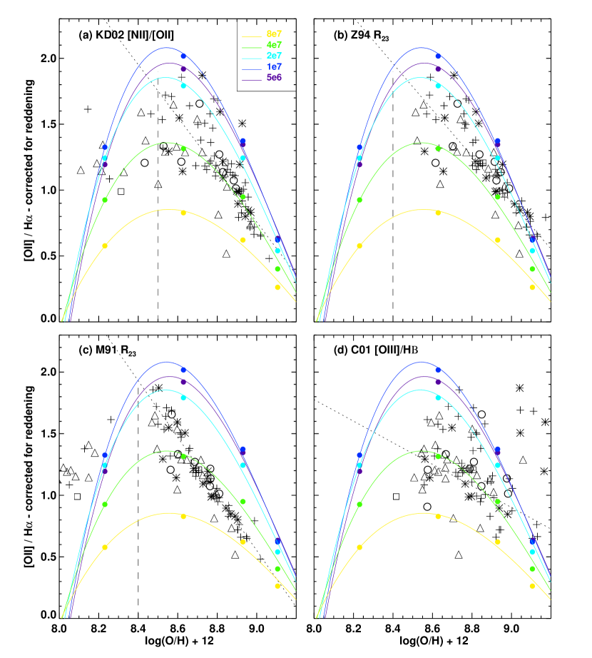
Figures (6a-d) show the relationship between the metallicity in units of log(O/H)+12 and [O II]/H (corrected for reddening) for the KD02, Z94, M91 and C01 abundance diagnostics respectively. The absolute values of the abundances vary depending on the diagnostic (Kewley & Dopita, 2002). The mean abundances are: (M91), (KD02 [N II]/[O II]), (C01), and (Z94). Note that the Z94 diagnostic is an overestimate because Z94 abundances cannot be calculated for galaxies with . The KD02 [N II]/[O II] diagnostic is also an upper limit because of the decreasing sensitivity of [N II]/[O II] with smaller abundances.
For metallicities (M91, Z94, C01 methods) and (KD02 method), we fit a least-squares line of best fit to the relationship between [O II]/H and abundance (dotted line in Figure 6). This line has the form:
| (7) |
where is the slope and is the y-intercept. Table 2 gives the slope, y-intercept, and rms for each of the four abundance diagnostics. Ideally, all diagnostics should produce the same estimate for the oxygen abundance for each galaxy. Unfortunately, abundance diagnostics are subject to systematic errors resulting from either the modeling, or the data used to calibrate the diagnostic (see Kewley & Dopita, 2002, for a review). These errors are particularly significant for the and [O III]/H diagnostics: and [O III]/H are double valued with abundance and are strongly influenced by the ionization parameter. Because of these errors, the observed relationship between [O II]/H and abundance is influenced by the shape of the model curves used to calibrate the diagnostics. The shape of the model curves demonstrate the theoretical temperature sensitivity of [O II] with increasing abundance. Because the linear relations are model-dependent, it is rather remarkable that for , the KD02 [N II]/[O II], M91 , and Z94 diagnostics have the same slope and y-intercept to within the errors. Table 2 lists the Spearman Rank coefficients and probabilities. For the M91, Z94 and KD02 methods, the correlation coefficient is , with the probability of obtaining such a correlation coefficient by chance . Because the M91, Z94, and [NII]/[OII] diagnostics are independent, we can be reasonably confident that the strong correlation observed between [O II]/H and abundance is real. Indeed, the ratio is a valid abundance diagnostic for precisely this reason. For the ionization parameter range of our sample, the shape of the curves derives from the temperature sensitivity of the [O II] emission-line compared to H. At high metallicities, is strongly sensitive to the metallicity because the [O II] and (to a lesser degree) [O III] fluxes drop dramatically with the low electron temperatures associated with the increasing abundance. However, at low metallicities (), the electron temperature is high and the [O II] flux increases slowly with abundance. The strong relationship between [O II]/H and metallicity should also be observed for metallicities derived from non- methods. Figure (6a) supports this statement: the [O II]/H ratio is strongly correlated with the oxygen abundance derived from [N II]/[O II]. The Spearman-Rank correlation coefficient is -0.79 and the probability of obtaining this value by chance is negligible (1.75). The slope and y-intercept for the [N II]/[O II]-derived abundances are within the error range for the other three diagnostics.
The C01 [O III]/H diagnostic, however, shows a considerably larger scatter, with an rms of 0.24 about the best-fit line. KD02 showed that the C01 “case a” ([N II]/[S II]) diagnostic also exhibits a larger scatter compared to the M91, Z94, or KD02 theoretical methods (including, but not limited to ). In addition to placing most galaxies at abundances , the C01 diagnostic also predicts that 16 galaxies have very low global abundances (). The C01 [O III]/H diagnostic appears to introduce a strong systematic effect in the abundance estimates. We will analyze this issue for the C01 diagnostic in Section 5.
4.4 SFR([O II]) and Oxygen Abundance Correction
In this section, we apply an abundance correction to our [O II] SFR calibration. SFR([O II]) is normally calibrated using an assumed [O II]/H ratio. This ratio is not independent of abundance. We have shown that the actual [O II]/H ratio varies considerably for the NFGS sample, and that this variation is strongly correlated with the oxygen abundance. For , the use of any particular [O II]/H ratio automatically implies a metallicity which may or may not be appropriate for the sample being studied.
Ideally, one should use the [O II]/H ratio for each galaxy to derive an SFR([O II]) diagnostic. However, if H were available, it would be used as an SFR diagnostic rather than [O II]. For redshifts , it is theoretically possible to use H as a SFR diagnostic through the SFR(H) calibration. In practice, H is often contaminated by an unknown amount of underlying stellar absorption. In the absence of H or a high S/N, high resolution H an oxygen abundance estimate can be used as a tracer of the [O II]/H ratio. To obtain the SFR([O II]), we start with the SFR(H) calibration derived by K98:
| (8) |
| (9) |
The SFR([O II]) spans four orders of magnitude and is therefore particularly sensitive to the values of and . Care should be taken to use , , and derived from the same abundance diagnostic (Table 2). This process assumes (1) that the relationship between [O II]/H and metallicity is linear, and (2) that the abundance diagnostic being applied is reliable. Both of these assumptions are only valid for metallicities where the [O II]/H emission decreases with increasing abundance. The [O II] flux is not a strong function of electron temperature at low metallicities because the nebular cooling is dominated by hydrogen free-free emission.
Figure 7 shows the relationship between the K98 H SFR and the SFR([O II]) derived from our new calibration (equation 9) for each of the abundance diagnostics. In each plot, a dotted line indicates the best fit to the data. Table 3 gives the slope, y-intercept, and rms for each fit. For comparison, Table 3 also lists the slope, y-intercept, and rms for the K98 SFR([O II]) and SFR(H) plot in Figure 2. After correction for oxygen abundance, in all four cases the line of best fit to the data has a slope of and a y-intercept of within the errors, indicating that the abundance correction does not introduce a systematic offset. For the KD02, M91 and Z94 diagnostics, the rms scatter decreases significantly after correction for oxygen abundance (0.03-0.05 versus 0.08-0.11).
Cardiel et al. (2003) also observed a decreased scatter after metallicity correction in a small sample of 7 galaxies with redshifts of and . Cardiel et al. applied a metallicity correction to [O II] based on and found excellent agreement between SFR([O II]) and SFR(H). This result gives us confidence that our abundance-corrected SFR([O II]) calibration will be applicable to more distant samples than the NFGS. Indeed, we derive our SFR([O II]) calibration only from the strong [O II]/H-metallicity correlation. In theory, this correlation is a result of the temperature sensitivity of [O II] relative to H and, therefore, should not be sensitive to redshift. In practice, however, the situation is more complicated. The abundance diagnostics are based on theoretical models calibrated against nearby H II regions or galaxies. It is unclear whether the model assumptions apply at high-. Model assumptions which may differ at high- include (but are not limited to) the gas geometry, dust geometry, density, and the initial mass function.

The large scatter (Figure 7d) for the C01 “case F” ([O III]/H) abundance diagnostic propagates into the SFR([O II]) calibration based on the C01 constants and abundance estimate. We therefore do not recommend the use of C01 case F to derive an abundance-corrected [O II] star formation rate if large scatter is a concern. As we have seen, the M91, Z94 and KD02 abundance diagnostic methods (and associated and constants) give almost identical relations (within the errors) between SFR(H) and SFR([O II]) with a very small scatter (0.03-0.05 dex). The fact that Z94, M91, and KD02 ([N II]/[O II]) are independent of one another and still produce identical relations (within the errors) supports the use of these to correct the NFGS [O II] SFRs for oxygen abundances between .
The drawback to using diagnostics is that they are double-valued with abundance. The M91 diagnostic requires an initial guess of the oxygen abundance to determine which branch of the curve to use. The Z94 calibration is only valid for the upper metallicity branch (). Unfortunately, the [O II], [O III], and H lines alone are not sufficient to determine which branch of the curve to use. For the NFGS sample, we use the [N II]/[O II] line ratio to resolve this problem. In local galaxies, the luminosity-metallicity (L-Z) correlation may help to break the degeneracy. For example, objects more luminous than generally have metallicities greater than (e.g., Z94) and therefore probably lie on the upper branch. Figure 8 supports this conclusion. In Figure 8, we compare the absolute magnitude for the NFGS galaxies with the abundances derived with the KD02 [N II]/[O II] and the M91 methods. Even though the KD02 [N II]/[O II] method is less sensitive to abundance for , the KD02 [N II]/[O II] method shows a strong correlation between abundance and . For abundances estimated using KD02, all eight galaxies with have . For abundances calculated using M91, 13/15 (87%) of the galaxies with have . For , therefore, is a useful discriminator between the two branches in nearby galaxies and provides a crude estimate of the abundance in the absence of alternative methods. The error in the abundance is likely to be in units of log(O/H)+12. At lower luminosities (), the -metallicity relation provides, at most, an upper limit.
It is not clear whether the same -metallicity relationship applies for galaxies at higher redshifts. The few studies of the luminosity-metallicity (L-Z) relation at larger redshifts appear to produce conflicting results. Carollo & Lilly (2001) analysed a sample of 13 star forming galaxies between and find no significant evolution in the L-Z relation out to . Lin et al. (1999) examined 2000 late-type CNOC2 (Canadian Network for Observational Cosmology Field Galaxy Redshift Survey) galaxies and found no significant luminosity evolution between . However, results from the DEEP Groth Strip Survey suggest that the L-Z relation does evolve from the local relation between to (Kobulnicky et al., 2003). At larger redshifts , the L-Z relation appears to be significantly different from the local relation (Kobulnicky & Koo, 2000; Pettini et al., 2001). Therefore, although potentially useful, the local -metallicity relationship should not be applied blindly to non-local samples.

To conclude, the Z94 abundance estimates agree well with those obtained using the KD02 [N II]/[O II] diagnostic. The [N II]/[O II] ratio is very sensitive to metallicity and is almost independent of ionization parameter (KD02). Therefore, if an initial guess of the abundance gives , and the ionization parameter is likely to cover a small range (similar to the NFGS or local H II regions), we recommend using the Z94 diagnostic. Using the slope and y-intercept appropriate for Z94 (Table 2) gives:
| (10) |
where comes from
| (11) |
and .
Given the difficulty in estimating abundances with limited data, our SFR([O II],Z) calibration should be useful for deriving an SFR([O II]) calibration for samples which have a different mean abundance from the NFGS. Equation (4) is based on the mean intrinsic [O II]/H of the NFGS sample. Any SFR([O II]) calibration that is derived from SFR(H) and an [O II]/H ratio automatically includes an assumption about the average abundance. As we have seen, the remaining cause of discrepancies in [O II]/H from galaxy to galaxy in the NFGS is abundance. If the mean abundance of a sample is not the same as for the NFGS (using the same abundance diagnostic), then equation (10) can be used to calculate a new SFR([O II]) calibration based on the mean or assumed abundance for the new sample. This approach could be useful in cases where individual galaxy abundances are not available, but an estimate of the sample mean abundance can be made. Such estimates could be based on known abundances for similar galaxies, or could be calculated using a subsample of galaxies for which abundance measurements are available (e.g., Lilly, Carollo, & Stockton, 2003). A similar process can be utilized for deriving a mean sample extinction estimate.
If no abundance estimate can be made, we recommend using equation (4) derived in Section 4.1. This SFR indicator is most useful for large samples because, provided the mean abundance is similar to that observed in the NFGS, the mean SFR([O II]) should approximate the mean SFR(H), thus reducing the scatter. Note that our equations (4) and (10) assume that the [O II]/H ratio does not depend significantly on the ionization parameter. Investigations using SFR([O II],Z) should also include a calculation of [O III]/[O II] to measure the dominant ionization state of oxygen. If [O III]/[O II] covers a wide range, and the oxygen abundance covers a relatively small range, then equation (4) would be a more appropriate SFR([O II]) calibration to use.
5 A Theoretical Calibration of SFR([O II]) and Abundance
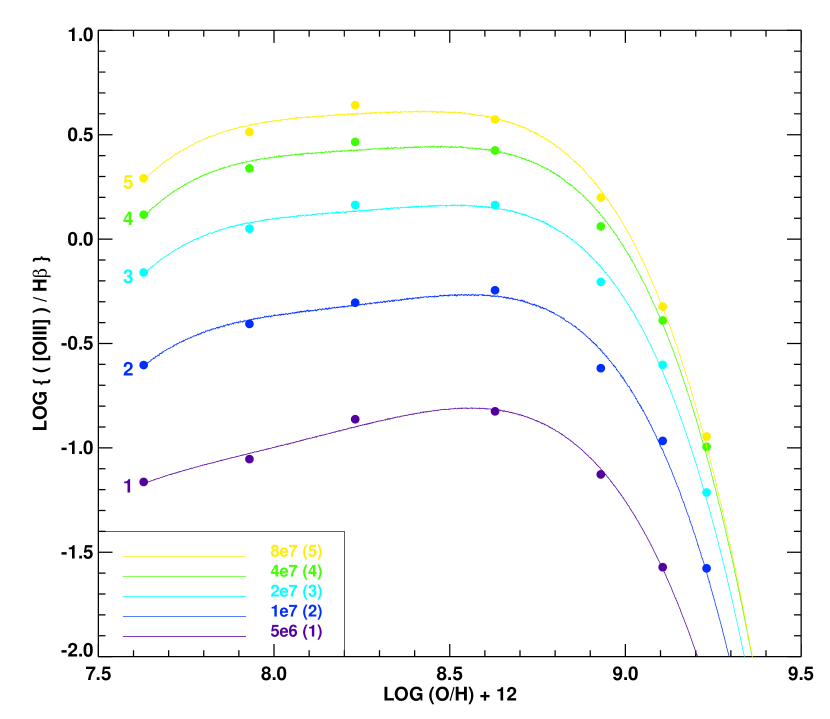
In this section, we utilize theoretical models to further investigate the relationship between the [O II]/H ratio, abundance, and the ionization state of the gas. We use the stellar population synthesis models Pegase (Fioc & Rocca-Volmerange, 1997) and Starburst99 (Leitherer et al., 1999) to provide the ionizing stellar radiation field for the photoionization code, Mappings III (eg., Sutherland & Dopita, 1993; Groves et al., 2003). Mappings III self-consistently calculates radiative transfer through gas in the presence of dust. Our models, described in Kewley et al. (2001b); Dopita et al. (2000), have been successfully applied to H II regions (Kewley & Dopita, 2002; Dopita et al., 2000) and nearby starburst galaxies (Kewley et al., 2001b; Calzetti et al., 2003). We use the instantaneous burst models with an ionization parameter range of cm/s. The models cover metallicities of 0.05, 0.1, 0.2, 0.5, 1.0, 1.5, 2.0, and 3.0solar, where solar metallicity is defined in Anders & Grevesse (1989). The corresponding metallicities in are 7.6, 7.9, 8.2, 8.6, 8.9, 9.1, 9.2, 9.4. Note that for the currently favored value of solar abundance (; Allende Prieto, Lambert, & Asplund, 2001), the model metallicities become 0.09, 0.2, 0.4, 0.9, 1.7, 2.6, 3.5, 5.2solar. The metallicities correspond to specific stellar tracks used in the population synthesis models and to the nebular abundance of the photoionization models. Typical metallicities for H II regions range between (e.g., Kewley & Dopita, 2002).
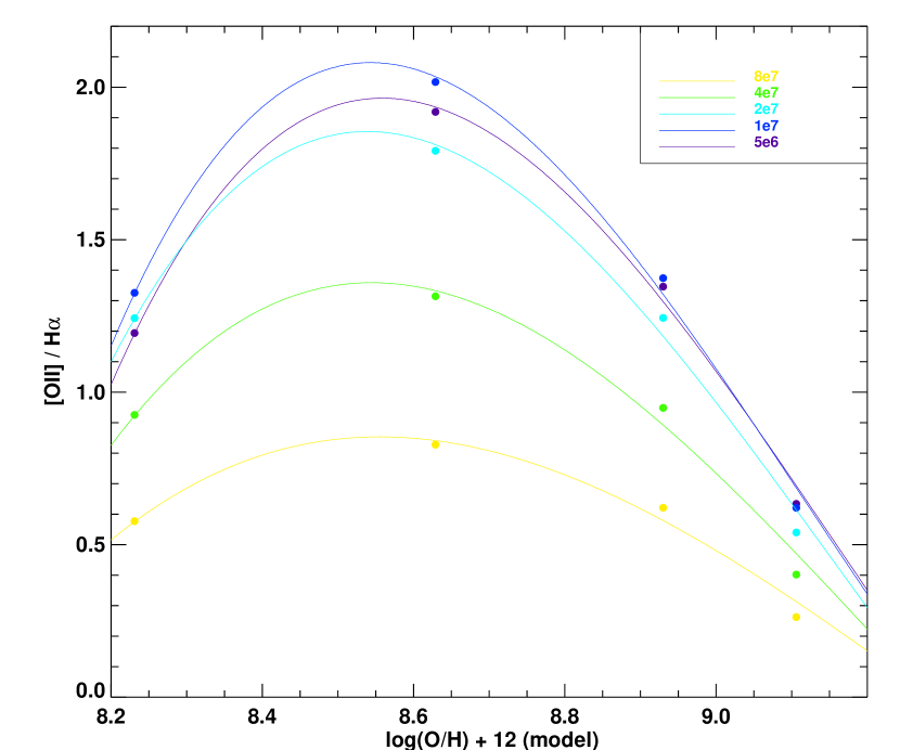
Figure 9 shows the theoretical relationship between [O II]/H and metallicity. We conclude that: (a) both ionization parameter and metallicity affect the [O II]/H ratio, and (b) for a particular sample, the relative importance of the ionization parameter compared to metallicity is governed by the range in abundances and ionization parameters spanned by the sample. The [O II]/H ratio is relatively insensitive to metallicity for . However, for , [O II]/H becomes a strong function of metallicity, particularly for low ionization parameters. This behaviour reflects the temperature sensitivity of the [O II] emission-line. As we have discussed, for temperatures typical of star-forming regions (10000-20000 K), the excitation energy between the two upper D levels for [O II] and the lower S level is of the order of the thermal electron energy . The [O II] doublet is therefore closely linked to the electron temperature. At low metallicities, the electron temperature is high, and [O II] emission increases with metallicity. In this regime, the thermal cooling is dominated by hydrogen free-free emission. However, when the metallicity increases, the number of coolants in the nebula rises, thus lowering the electron temperature. The [O II] emission therefore drops rapidly with increasing metallicity.
Figure 9 predicts that samples covering a small range of metallicities will not show a correlation between [O II]/H and abundance because of the range of possible ionization parameters. Samples spanning metallicities will also not show a strong relationship between [O II]/H and because at these metallicities [O II]/H is a weak function of and [O II]/H is more strongly affected by the ionization parameter. Only samples with a normal range of ionization parameters (cm/s; Dopita et al., 2000) and covering a large range of metallicities exceeding will exhibit a correlation between [O II]/H and metallicity.
Note that our models do not require a specific method for calculating metallicities from the data. If the metallicities are calculated using some reliable abundance diagnostic, our models predict that galaxies with typical ionization parameters and metallicities lie along the curves in Figure 9. The curve for each ionization parameter can be characterized by a third order polynomial:
| (12) |
where and the coefficients are displayed in Table 4.
In Figure (10), we compare the theoretical models with the abundances derived using the different diagnostics. In Figure (10a) we show the abundances derived using [N II]/[O II]. The ionization parameters are typically cm/s , and the data follow a similar trajectory to the models. As we have discussed, the oxygen abundances derived using the [N II]/[O II] diagnostic show a larger scatter, particularly for oxygen abundances . The models show that the [N II]/[O II] and [O II]/H ratios become less sensitive to abundance as metallicity decreases, increasing the scatter. The Z94 method produces abundances similar to the [N II]/[O II] method. The data follow a similar trajectory to the models and the ionization parameters are between typically cm/s.
The M91 method (Figure 10c) shows a systematic offset compared to the Z94 and KD02 methods and to the models. This offset has been observed previously (Kewley & Dopita, 2002) and is probably a result of the different stellar atmospheres and stellar models used to derive the ionizing radiation fields. The difference in abundances estimated for the M91 and KD02 method is in . This variation is within the errors associated with the diagnostics (0.15 dex for M91 and 0.1 for KD02). We note that the diagnostics may be minimizing the scatter by making a hidden assumption about the ionization parameter. The ratio is sensitive to the ionization parameter and the ionization parameter diagnostic [O III]/[O II] is sensitive to abundance. If the ionization parameter correction is not made iteratively, then a calibration may, in effect, favor a particular ionization parameter or range of ionization parameters. This effect may contribute to the difference between the M91 and Z94 diagnostics. The Z94 abundance estimates agree well with the ionization-parameter independent diagnostic [N II]/[O II].
The C01 “case F” diagnostic produces some [O II]/H-abundance combinations which can not be produced using our stellar population synthesis+photoionization models, even with the 0.1 dex error estimates. As we discussed earlier, the C01 “Case F” diagnostic is based on [O III]/H for the majority of galaxies in our sample. Figure 11 shows the theoretical relationship between [O III]/H and abundance. The [O III]/H ratio is much more sensitive to the ionization parameter than metallicity for all but the highest metallicities. In addition, [O III]/H is double valued with abundance. Any particular [O III]/H ratio could correspond to a range of abundance/ionization parameter combinations, and the possibility of obtaining an incorrect abundance estimate is high.
We can conclude from Figures 10a-c that the [O II]/H ratio depends on abundance for , and that a linear correction for abundance is theoretically plausible for samples with metallicities in this range, providing the data do not span a larger range in ionization parameters than is observed in local H II regions. For the KD02, Z94, and M91 abundances, the NFGS data follow a trajectory with a similar slope to the models for . The model trajectory for each ionization parameter can be used to derive a theoretical [O II] SFR calibration. We begin, once again, with the K98 SFR(H) calibration:
| (13) | |||||
| (14) |
where the constants are given in Table 4 for each ionization parameter and . The subscript indicates that the calibration is based on theoretical models. The majority of the NFGS have ionization parameters between cm/s, according to the KD02 [N II]/[O II] and Z94 diagnostics. Interpolating between the and 4cm/s curves gives a curve with an approximate ionization parameter of cm/s:
| (15) |
This curve provides a useful theoretical description of the behavior of [O II]/H with metallicity for the NFGS sample. We emphasize that the metallicities of the models correspond to the metallicities in the stellar tracks and the modeled nebulae, and are independent of the method used to derive . Therefore, any method can be used to derive , as long as the method is reliable over the expected abundance range of the sample. The Z94 diagnostic can easily be used if the abundances exceed .
In Figure 12, we compare the H and [O II] SFRs with SFR([O II],Z) calculated according to our theoretical models (equation 15) with abundances estimated by either (a) the KD02 [N II]/[O II] method or (b) the Z94 method. Table 3 contains the slope, intercept, and scatter. The slope and y-intercept are close to unity and zero respectively, for both abundance diagnostics. The scatter is 0.05 dex compared to 0.08 dex using our SFR([O II]) calibration without correction for abundance (equation 4; Figure 4). Clearly our theoretical SFR([O II],Z)t calibration is successful in reducing the scatter observed in the SFR([O II]) estimates. This diagnostic will be most useful for deriving a new SFR([O II]) calibration for samples which have a different mean abundance from the NFGS.

6 The application of SFR([O II]) to high galaxies
6.1 Reddening Determination
Recently, many investigations have used [O II] to constrain the cosmic star formation history for redshifts (e.g., Hammer et al., 1997; Hogg et al., 1998; Rosa-Gonzàlez, Terlevich, & Terlevich, 2002; Hippelein et al., 2003). At these redshifts, H is usually unavailable and correction for reddening using the methods outlined above is thus impossible. Without the Balmer decrement, many investigators apply an “average” or “recommended” mean attenuation of mag prior to the calculation of either SFR([O II]) or abundance. Assuming , corresponds to E(. Figure 13 shows the distribution of reddening traced by E(B-V) for our sample. The mean E(B-V) for the galaxies in our sample (after correction for Galactic extinction) is , consistent with the common choice of E(.

If we apply an E( to and L([O II]) and use equations (10)-(11) or equation (15) to derive the SFR, the slope is (Figure 14a,b). Thus, with a single E() the SFR([O II]) is a systematic underestimate at high SFRs and a systematic overestimate at low SFRs. This effect would be observed if the galaxies at the highest SFRs are more highly extincted than galaxies with lower SFRs. Wang & Heckman (1996) showed that the reddening (measured using the H/H ratio) correlates with FIR luminosity for a sample of nearby disk galaxies. A similar effect appears in a sample of nuclear starburst and blue compact galaxies by Calzetti et al. (1995). We also know from Kewley et al. (2002) that the SFR(FIR) agrees to within 10% on average with SFR(H), and we have shown here that there exists a 1:1 relationship between SFR(H) and SFR([O II]) after reddening and abundance correction. It is therefore not surprising that we observe increasing reddening with SFR([O II]).


Figure 15 shows a strong correlation of L([O II]) with E(B-V) for our sample with a large scatter (rms=0.13 dex). We corrected L([O II]) for reddening using the Balmer decrement. The Spearman Rank coefficient is 0.73; the probability of obtaining this coefficient by chance is . We made two fits to the data to estimate the impact of the upper limits: one with the upper limits on E(B-V) set at their maximum value of 0.02 (dashed line in Figure 15), and the second line with the upper limits set at zero (dot-dashed line). The fits are almost identical: the slope and y-intercepts agree to within 1%, well within the errors. The best fit (including E(B-V) upper limits as either 0.02 or 0.00) is:
| (16) |
where the subscript i indicates that L([O II]) (in ergs/s) has been corrected for reddening. The intrinsic [N II] luminosity is also correlated with E(B-V) (Figure 15). The [N II] emission-line requires less correction for reddening than [O II] and provides an independent measure of the relationship between the emission-line luminosity and reddening for the NFGS sample.
This relationship can be understood physically: the galaxies with the highest rates of star formation are likely to also produce larger quantities of dust. Most of the dust in galaxies is probably produced by carbon or oxygen-rich stars on the asymptotic giant branch (see Mathis, 1990, for a review). Supernovae may also be important because they insert heavy elements into the surrounding interstellar medium. If we assume that the initial mass function is similar for the galaxies in our sample, then higher star formation rates enable more carbon and oxygen-rich stars to reach the asymptotic giant branch, producing larger quantities of dust. This scenario implies that most of the NFGS galaxies must have been forming stars at least 1.5-2 Gyr ago because it takes approximately this long for the low- and intermediate-mass stars in a typical stellar population to evolve to the asymptotic giant branch (e.g., Mouhcine & Lancon, 2002).
The scatter around the fit in Figure 15 is large (0.13 dex). The amount of dust obscuring the observed optical emission from the nebular gas varies from galaxy to galaxy. In addition, because we use global spectra, we observe the sum of the emission from the brightest H II regions in each galaxy. Geometry, dust composition, and stellar properties are all likely to have an impact on the observed optical emission from the brightest H II regions.
Because the reddening is correlated with the intrinsic [O II] luminosity, equation (16) provides a very crude estimate of the reddening for the NFGS. The relationship between E(B-V) and the [O II] luminosity could be different for other samples and tests are required to determine whether equation (16) may be applied to non-NFGS galaxies. In addition, for galaxies at high redshift E(B-V) may not be a reliable indicator of the reddening if the dust does not conform to a foreground screen geometry (Witt & Gordon, 2000). However, there is some evidence that a reddening-luminosity relationship exists at high redshifts, at least for rapidly star-forming galaxies. Adelberger & Steidel (2000) found that the sum of the bolometric dust luminosity and the 1600Å luminosity () is correlated with the ratio of these two quantities () for high- and low- galaxies alike. The sum provides a crude estimate of the star formation rate; the ratio is a rough tracer of the dust obscuration. If such a reddening-luminosity relationship holds for non-NFGS samples, then it might be feasible to use equation (16) to derive a very rough reddening estimate at distances where H is redshifted out of the observable wavelength range.
The intrinsic [O II] luminosity is related to the observed [O II] luminosity using the standard equation (e.g., Calzetti et al., 2000):
| (17) |
where using the CCM reddening law. If we substitute equation (16) into equation (17) for E(B-V), we obtain:
| (18) |
where the intrinsic and observed luminosities are in units of ergs/s. The estimated intrinsic luminosity from equation (18) can now be used in equation (10) along with to calculate the SFR([O II],Z) for the NFGS. We emphasize that this relation may be different for other samples, and should not be applied blindly to other galaxies.

Figure 16 compares SFR([O II],Z) with SFR(H) for the NFGS, where SFR([O II],Z) is effectively corrected for reddening and abundance in the following manner:
-
1.
We estimate the intrinsic luminosity from equation (18).
-
2.
We estimate E(B-V) from the intrinsic luminosity with equation (16).
-
3.
We use the E(B-V) estimate to correct the ratio for reddening.
-
4.
We use the reddening-corrected ratio in the Z94 diagnostic (equation 11) to derive the abundance.
-
5.
We use the abundance and intrinsic luminosity in equation (10) to derive a reddening and abundance corrected SFR([O II],Z) estimate.
-
6.
We use the abundance and intrinsic luminosity in equation (15) to derive a reddening and abundance corrected SFR([O II],Z)t estimate from our theoretical SFR([O II],Z)t calibration.
Note that we correct the comparison star formation rate SFR(H) for reddening using the true E(B-V) obtained from the Balmer decrement. The best-fit lines in Figure 16 have a slope and a y-intercept close to zero (). Clearly, if the best-fit slope is not close to 1 (as is the case when an average A(v)=1 is assumed), the difference between the mean estimated SFR and the true SFR increases with increasing star formation rate. Thus the bias introduced can easily appear as a function of redshift because we observe intrinsically more luminous galaxies at larger . The scatter in Figure 16 is 0.21 dex but this scatter is less important than the slope for studies of the star formation history.
Figure 17 shows a comparison of the SFR(H) with the SFR([O II]) where SFR([O II]) is effectively corrected for reddening but only partially for oxygen abundance through the correlation of E(B-V) with luminosity. We calculated the intrinsic luminosity using equation (18), and derived the SFR([O II]) using equation (4). The scatter is larger than if we apply an abundance correction ( dex vs. 0.21 dex), but again, with large samples this increased scatter should not be a problem.

As we have stressed, our equations 4 and 10 were derived from an unbiased local sample. The excitation and abundance properties of galaxies in other samples and of galaxies at higher redshifts may not be the same as those observed in the local galaxy population. It may be possible to correct for reddening using a reddening-luminosity relation such as equation 18, but the application of equation 18 (or other such relation) awaits further testing. The lack of samples with both integrated spectra and Balmer decrement measurements (or other reddening indicator) make testing equation 18 difficult at present. We will test the reddening-luminosity relation for a large, objectively selected sample of galaxy pairs in a future paper (Kewley et al. in prep), once aperture effects have been analysed. For the reasons outlined above, we do not apply equation 18 to high- galaxies. Instead, we test whether our SFR([OII]) relations can be applied to galaxies at higher redshifts with the standard assumption of . Evidence for a mean for galaxies with redshifts is found by Tresse et al. (2002), Sullivan et al. (2000), Liang et al. (2003) using the Balmer decrement. However Flores et al. (1999) concludes that the global opacity of the () universe is between using radio, IR, UV, and optical photometry.
6.2 Testing SFR([OII]) for galaxies
To test our SFR([OII]) relations on galaxies at larger-, we use two samples: the sample of Hicks et al. (2002) (hereafter H02) and the sample of Tresse et al. (2002) (hereafter T02). H02 obtained rest-frame blue spectra for 14 emission-line galaxies representative of the population at in the 1999 NICMOS parallel grism H survey. We use the seven objects in H02 with measured [O II] and H luminosities. T02 obtained H measurements for 30 galaxies in the Canada-France Redshift Survey with redshifts . Both H02 and T02 report [O II]/H ratios that differ significantly from those in the NFGS, due either to much larger reddening values or intrinsically lower line ratios. Therefore, these samples provide a critical test of the applicability of our [O II]–SFR calibration to galaxies at higher redshifts.
We recalculated the [O II] and H luminosities for the standard cosmology (; ) and computed the intrinsic [O II] and H luminosities with the CCM reddening curve, assuming . Table 5 lists the relevant derived quantities. The SFR(H) and SFR([O II]) are from equations 1 and 4. SFR([O II]) is significantly lower than SFR(H) (Figure 18a). This discrepancy may result from one or a combination of (1) poor () S/N at [O II], (2), sky contamination at [O II], (3) a stronger dependence of [O II]/H on the ionization parameter than observed in the NFGS, (4) reddening more than the assumed , (5) reddening may not be a simple forground screen for the H02 and T02 galaxies, (6) the H02 and T02 samples may have a different mean oxygen abundance than the NFGS. We discuss these possibilities individually below.
6.2.1 Poor S/N
Poor S/N at [O II] may affect the H02 sample: only two H02 galaxies have [O II] detections. However, the majority (28/30) of the T02 sample have detections, ruling out poor S/N as a reason for the SFR discrepancy for the majority of galaxies in Figure (18a).
6.2.2 Sky Contamination
Sky contamination at [O II] affects the majority (5/7 galaxies) of the H02 sample, but the T02 sample was specifically selected to avoid sky contamination in the optical and near-IR. Inspection of the T02 spectra reveals no evidence for sky contamination.
6.2.3 Ionization Parameter
Ionization parameter estimates can not be made with the T02 and H02 samples because [O III] emission-line fluxes are unavailable. However, [O II] and [O III] fluxes are available for the sample by Lilly, Carollo, & Stockton (2002, 2003) (hereafter LCS). The mean [O III]/[O II] ratio for the LCS sample is , corresponding to a mean ionization parameter of cm/s using the [O III]/[O II] ionization parameter calibration of Kewley & Dopita (2002). If the mean ionization of the H02 and T02 sample is similar to that observed by LCS, then the ionization parameter cannot account for the SFR discrepancy in Figure (18a).
6.2.4 Reddening
If the SFR discrepancy is a result of reddening, then the average extinction required to bring the SFRs into agreement is . The variation in optical extinction as a function of redshift is unknown, however the multiwavelength study by Flores et al. (1999) suggests a mean extinction in galaxies of , significantly lower than .
6.2.5 Foreground Screen Assumption
An alternative explanation for the difference between the [O II] and H SFRs in Figure (18a) is that the dust geometry may not be a simple screen. Witt & Gordon (2000) show that E() saturates at around 0.2-0.3 mag for geometries where the dust is mixed with the gas. In this scenario, the true reddening may be much larger than predicted by E(). We will investigate this possibility in a future study of an unbiased sample of galaxy pairs and N-tuples (Barton, Geller, & Kenyon, 2000).
6.2.6 Metallicity
To investigate the effect of metallicity, we begin with the mean intrinsic [O II]/H ratios: and for the H02 and T02 samples, respectively (assuming an average mag). Using our theoretical grids (equation 12) and assuming that the average ionization parameter is cm/s, the H02 and T02 [O II]/H ratios correspond to metallicities of and using our theoretical models, or and using the M91 diagnostic and equation 7. These values are consistent with the recent result by LCS that % of 65 CFRS galaxies between have an oxygen abundance using the M91 method. The SFR([O II]) calibration used in Figure 18a assumes that the mean abundance is the same as that measured for the NFGS. The absolute value of the abundance is diagnostic dependent (compare the x-axes in Figures 6a - 6d). Because LCS use the M91 method, we also use this method to derive the mean NFGS abundance for comparison: . The difference between the NFGS, T02 and H02 metallicities is likely to result from the different luminosity ranges covered by each sample. Most high- samples consist of more intrinsically luminous galaxies than in local samples. Indeed, when LCS compare the mean abundances for the CFRS sample with the NFGS selected over the same luminosity range, they find that the mean abundances are similar.
Hydrodynamic cosmological models yield different predictions about the stellar metallicity distribution as a function of redshift. Models by Edvardsson et al. (1993) and Nagamine et al. (2001) predict that the average stellar metallicity is constant up to ; the models by Rocha-Pinto et al. (2000) predict that earlier stars are more metal-poor. Either way, it is likely that most samples observed at high- contain more intrinsically luminous (and thus higher metallicity) galaxies than local samples.
To check whether the high metallicities result from a luminosity selection effect, we compare the mean and metallicity with the metallicity-luminosity relations presented in Kobulnicky et al. (2003). The mean () and metallicity () for the T02 sample are consistent with the metallicity-luminosity relation for the DGSS galaxies in Kobulnicky et al. On the other hand, the H02 mean ( and metallicity () are more similar to the upper end of the luminosity-metallicity relation in local samples. This result may be caused by the H02 H sample selection. Such a selection could potentially bias the sample towards galaxies with intrinsically strong H fluxes, small [O II]/H ratios and high metallicities.
We obtain a metallicity-corrected SFR([O II]) with either the mean [O II]/H ratios and equation (1), or equivalently, we use the mean metallicities derived above and equation (15) or (10). Figure (18b) compares the metallicity-corrected SFR([O II]) estimates to SFR(H). The SFR([O II]) and SFR(H) agree with a mean relative scatter of 0.17 dex. We conclude that correcting for a mean metallicity consistent with the mean [O II]/H for the T02 and H02 samples produces better agreement between SFR([O II]) and SFR(H). The scatter is identical to that observed for the NFGS with mag (Figure 14).

7 SFR([O II]) and the Cosmic Star Formation History
Analysis of the star formation history of the Universe depends on use of the [O II] emission-line as a SFR diagnostic in the range (e.g., Hammer et al., 1997; Hogg et al., 1998; Sullivan et al., 2000; Gallego et al., 2002; Hippelein et al., 2003; Teplitz et al., 2003). There are many approaches to calculating the star formation history based on the [O II] luminosity. One approach (Hogg et al., 1998) is to calculate the [O II] luminosity density as a function of redshift and then to convert this estimate directly into a star formation rate based on one of the SFR([O II]) conversions. Hogg et al. use the K92 calibration, and conclude that it (the K92 conversion) may not be directly applicable to galaxies at high-.
Hippelein et al. (2003) take another approach. Hippelein et al. use an extinction-corrected [O II]/H flux ratio (0.9) to convert the K98 H SFR calibration into an [O II] SFR calibration for their sample which covers the redshift range . The resulting constant used to convert the intrinsic [O II] luminosity (in ergs/s) into a SFR is . If the [O II]/H ratio that Hippelein et al. derive is a good approximation to the average for their entire sample, then the constant may be used to predict a mean abundance. Equation (10) gives a mean abundance of for the Hippelein et al. sample with the M91 abundance diagnostic. This abundance estimate is similar to the mean abundance of the LCS sample (), and is reasonable if the Hippelein et al. sample contains relatively more luminous galaxies than in local samples. An alternative explanation of the low [O II]/H ratio observed by Hippelein et al. is that the ionization state of the gas dominates the [O II]/H ratio and that the average ionization parameter is higher in the Hippelein et al. sample than in the NFGS.
Teplitz et al. (2003) followed a similar method for their sample of 71 galaxies from the STIS Parallel Survey. They used the Jansen, Franx, & Fabricant (2001) NFGS relation between absolute blue magnitude and [O II]/H to derive an [O II]/H ratio (uncorrected for reddening) for various luminosity ranges in their sample. Teplitz et al. note that the [O II]/H ratio is highly dependent on the metallicity and reddening of each individual galaxy. Teplitz et al. calculate a mean uncorrected [O II]/H ratio of 0.45, lower than those observed locally (Figure 3a). From these ratios they convert the [O II] luminosity into an H luminosity using the K98 SFR(H) relation. Teplitz et al. show that the comoving star formation density estimated using H systematically exceeds the [O II] estimate derived for the same redshift range. However, Teplitz et al. use SFR densities which have been corrected for reddening in various ways. They use the uncorrected [O II] luminosity densities with the empirically derived [O II]/H to convert the [O II] luminosity densities into H luminosity densities. This process is similar to the one used by K98 to derive his SFR([O II]) indicator: the difference in reddening at [O II] and at H is taken into account, but the reddening of the H luminosity is not. The derived luminosity densities should therefore be corrected for reddening to allow comparison of the resulting SFR densities with those calculated from H surveys. Typically, H surveys are already corrected for reddening based on some assumption about the average attenuation. Many studies of SFR densities based on H make a correction for reddening based on an assumed mag.

Figure (19a) shows the discrepancy observed by Teplitz et al. (2003) between star formation densities measured with H and those measured with [O II]. All data on Figure (19) have been converted to the standard cosmology (, ; Table 6). Some of the SFR densities from Figure (19a) have been corrected or partially corrected for reddening; others are uncorrected.
Gallego et al. (2002) emphasize the importance of using the same assumptions for star formation rate conversion and reddening for all data points in SFR density comparisons. For example, Figure (5) in Teplitz et al. (2003) and Figure (19a) show that the H SFR density point of Pascual et al. (2001) significantly exceeds that of Tresse & Maddox (1998). The source of this apparent difference is in the assumed reddening. Pascual et al. (2001) use an which corresponds to an E(B-V) and an attenuation factor of ; Tresse et al assume an average which corresponds to an E(B-V), corresponding to an average attenuation of . If we assume the same reddening of for both samples, the two H SFR density estimates agree to within 10% (see Figure 19b).
Figure (19a) also shows [O II] SFR densities, including those by Hammer et al. (1997). Because Hammer et al. provide the comoving luminosity density (uncorrected for reddening) as a function of redshift, we convert these into reddening corrected SFR densities using our SFR([O II]) formula (equation 4), assuming an average reddening of . Figure (19b) shows the new SFR([O II]) densities. The resulting intrinsic SFR([O II]) densities are % larger than the SFR([O II]) densities in Figure (19a), bringing the SFR([O II]) values into closer agreement with the SFR(H) data points. This difference is a result of reddening correction. This conclusion can easily be verified by correcting the SFR(H) densities (calculated by Teplitz et al. using the Hammer et al. data and [O II]/H) for reddening at H using the same extinction curve and assuming an . Even with a 50% increase, the [O II] SFR density estimates are still lower than the H SFR estimates, reminiscent of the T02 and H02 galaxies in Section 6.
So far, we have used equation (4) to estimate the SFR([O II]) densities. The use of this equation assumes that the average abundance for the samples at high- is (M91 diagnostic) as observed in the NFGS. The LCS sample, and most other high-z samples, contain many intrinsically more luminous galaxies than in the NFGS. Galaxies with luminosities representative of the local luminosity function are often too faint to be included in high redshift samples. As we have discussed, the star formation rate density for any particular redshift is estimated using the [O II] luminosity density and some [O II] SFR calibration. The use of any SFR [O II] calibration requires the calculation of or an assumption about the [O II]/H ratio. In SFR history studies, the luminosity density is, in principle, corrected for the missing lower luminosity galaxies but the assumed [O II]/H is not corrected. The [O II]/H ratio for high- samples will be typical of the high luminosity (high-metallicity) galaxies observable, despite the fact that the mean metallicity for high redshift galaxies must actually be lower than is observed locally. Evidence for an [O II]/H ratio typical of high luminosity galaxies is easily observed in the Hippelein et al. and Teplitz et al. samples. The mean reddening-corrected [O II]/H ratio for the Hippelein sample (0.9) corresponds to a mean abundance of (M91 method). The Teplitz sample has a mean uncorrected [O II]/H ratio of . If we assume an (as in Tresse et al., 2002; Pascual et al., 2001), then the mean reddening-corrected [O II]/H ratio is . This [O II]/H ratio corresponds to a mean metallicity of , similar to the Hippelein sample.
Both Teplitz et al. and Hippelein et al. use an [O II]/H ratio typical for high- galaxies in their SFR density calculation. This [O II]/H ratio effectively takes the average metallicity into account. We should therefore apply a similar correction. If we assume that the average oxygen abundance for the Hammer et al. and Teplitz et al. galaxies is (using the M91 method) then equation 4 becomes:
| (19) |
where we have assumed the NFGS rms dispersion about the mean abundance. The L([O II]) is corrected for reddening assuming and a foreground screen geometry. The resulting SFR densities are a factor of 1.45 larger than the estimates with equation (4). The [O II] SFR density estimates are still slightly lower than the H SFR density estimates, but the the H and [O II] SFR densities now agree to within % (Figure 19c).
An alternative explanation for the difference between the [O II] and H SFR densities in Figure 19b is that the dust geometry may not be a simple screen. Witt & Gordon (2000) show that E() saturates at around 0.2-0.3 mag for geometries where the dust is mixed with the gas. In this scenario, the true reddening may be much larger than predicted by E().
We conclude that the major differences between H and [O II]-based estimates of the star formation rate density as a function of redshift probably result from inconsistent assumptions about reddening and abundance, and/or from failure to correct for the biases they introduce. Careful correction for both the reddening and abundance brings the star formation rate density estimates into agreement to within %.
8 Conclusions
We investigate the use of the [O II] emission-line as a star formation indicator for a sample of 97 nearby field galaxies. Our high S/N integrated (global) spectra allow correction of the Balmer lines for underlying stellar absorption and correction of the emission-line fluxes for abundance. We find:
-
•
There is a systematic difference between the SFR(H) and SFR([O II]) using the Kennicutt (1998) calibrations. The difference results from the use of the observed (uncorrected) [O II]/H ratio to convert the [O II] luminosity into a SFR indicator.
-
•
We derive a new SFR([O II]) indicator (equation 4) which is independent of the reddening between [O II] and H. This indicator removes the systematic difference observed for the Kennicutt calibration.
We estimate the abundances for our sample using four independent abundance diagnostics: Kewley & Dopita (2002) ([N II]/[O II]), McGaugh (1991) (), Zaritsky, Kennicutt & Huchra (1994) (), and Charlot & Longhetti (2001) ([O III]/H). We show that:
-
1.
There is a strong correlation between abundance and the [O II]/H ratio.
-
2.
There is no strong dependence of [O II]/H on the ionization parameter for
-
3.
The observed discrepancy between the Kennicutt (1998) SFR(H) and SFR([O II]) calibrations result from reddening and abundance differences between the K92 sample and other surveys.
Our theoretical stellar population synthesis and photoionization models support these conclusions. We derive a new SFR([O II],Z) calibration which includes a correction for abundance (equation 10). This relation reduces the rms residuals between SFR(H) and SFR([O II]) significantly from 0.11 to 0.03-0.05 dex. Our SFR([O II],Z) calibration is based on the intrinsic (reddening corrected) [O II] luminosity and the abundance. This calibration can be used to derive a SFR relation for samples where the mean abundance differs from the NFGS. The SFR([O II],Z) relation may also be applied to samples where abundance estimates are available, but where H has too low a S/N to be used to calculate a star formation rate based on H.
We observe a strong correlation between the intrinsic [O II] luminosity and E(B-V) for the NFGS. Using the observed [O II] luminosity to estimate the reddening produces no systematic shift between the SFR(H) and SFR([O II]), but there is a large dispersion (0.21 dex). Further investigation is required to verify whether a similar reddening-luminosity relation holds for other samples.
We discuss the application of our SFR([O II]) calibrations to studies of the cosmic star formation history. We show that we can remove the previously observed discrepancy between the star formation rates based on [O II] and those based on H by correcting for reddening and abundance. The agreement between SFR(H) and SFR([O II],Z) emphasizes the importance of aquiring data which yield internally consistent reddening and abundance estimates over the entire redshift range of the sample.
References
- Adelberger & Steidel (2000) Adelberger, K. L. & Steidel, C. C. 2000, ApJ, 544, 218
- Allende Prieto, Lambert, & Asplund (2001) Allende Prieto, C., Lambert, D. L., & Asplund, M. 2001, ApJ, 556, L63
- Anders & Grevesse (1989) Anders, E. & Grevesse, N. 1989, Geochim. & Cosmochim. Acta 53, 197
- Aragón-Salamanca et al. (2003) Aragón-Salamanca, A., Alonso-Herrero, A., Gallego, J., García-Dabó, Pérez-González, P. G., Zamorano, J., Gil de Paz, A. 2003, astro-ph/0210123
- Baldry et al. (2002) Baldry, I. K., et al. 2002, ApJ, 569, 582
- Barton, Geller, & Kenyon (2000) Barton, E. J., Geller, M. J., & Kenyon, S. J. 2000, ApJ, 530, 660
- Buat et al. (2002) Buat, V., Boselli, A., Gavazzi, G. & Bonfanti, C. 2002, A&A, 383, 801
- Burnstein & Heiles (1984) Burnstein, D. & Heiles, C. 1984, ApJS, 54, 33
- Cardelli, Clayton, &Mathis (1989) Cardelli, J. A., Clayton, G. C., & Mathis, J. S. 1989, ApJ, 345, 245
- Cardiel et al. (2003) Cardiel, N., Elbaz, D., Schiavon, R. P., Willmer, C. N. A., Koo, D. C., Phillips, A. C., Gallego, J. 2003, ApJ, 584, 76
- Calzetti et al. (1995) Calzetti, D., Bohlin, R. C., Kinney, A., Storchi-Bergmann, T., & Heckman, T. 1995, ApJ, 443, 136
- Calzetti et al. (2000) Calzetti, D., Armus, L., Bohlin, R. C., Kinney, A. L., Koorneef, J., & Storchi-Bergmann, T. 2000, ApJ, 443, 136
- Calzetti et al. (2003) Calzetti, D., Harris, J., Gallagher, J. S. III, Smith, D. A., Conselice, C. J., Homeier, N., & Kewley, L. 2003, ApJ, submitted
- Carollo & Lilly (2001) Carollo, C. M. & Lilly, S. J., 2001, ApJ, 548, L153
- Charlot & Longhetti (2001) Charlot, S. & Longhetti, M. 2001, MNRAS, 323, 887
- Charlot et al. (2002) Charlot, S., Kauffman, G., Longhetti, M., Tresse, L., White, S. D. M., Maddox, S. J., & Fall, S. M. 2002, MNRAS, 330, 876
- Cole et al. (2001) Cole, S. et al. 2001, MNRAS, 326, 255
- Cowie et al. (1997) Cowie, L. L., Hu, E. M., Songaila, A., & Egami, E. 1997, ApJ, 481, L9
- Davis & Peebles (1983) Davis, M. & Peebles, P. J. M. 1983, ApJ, 267, 465
- de Vaucouleurs et al. (1991) de Vaucouleurs, G., de Vaucouleurs, A., Corwin, H. G., Jr., Buta, R. J., Paturel, G., & Fouqué, P. 1991, Third Reference Catalogue of Bright Galaxies (New York: Springer)
- Donas & Deharveng (1984) Donas, J. & Deharveng, J. M. 1984, A&A, 140, 325
- Dopita & Evans (1986) Dopita, M.A. & Evans, I.N. 1986, ApJ, 307, 431
- Dopita et al. (2000) Dopita, M. A., Kewley, L. J., Heisler, C. A., & Sutherland, R. S. 2000, ApJ, 542, 224
- Dopita et al. (2002) Dopita, M. A., Periera, L., Kewley, L. J., & Capacciolo, M. 2002, ApJS, 143, 47
- Edmunds & Pagel (1984) Edmunds, M.G. & Pagel, B.E.J. 1984, MNRAS, 211, 507
- Edvardsson et al. (1993) Edvardsson, B., Anderson, J., Gustafsson, B., Lambert, D. L., Nissen, P. E., & Tomkin, J. 1993, A&A, 275, 101
- Ellis et al. (1996) Ellis, R. S., Colless, M., Broadhurst, T., Heyl, J., Glazebrook, K. 1996, MNRAS, 280, 235
- Ferland & Truran (1981) Ferland, G. J. & Truran, J. W. 1981, ApJ, 244, 1022
- Fioc & Rocca-Volmerange (1997) Fioc, M., & Rocca-Volmerange, B. 1997, A&A, 326, 950
- Flores et al. (1999) Flores, H., Hammer, F., Thuan, T. X., Césarsky, C., Desert, F. X., Omont, A., Lilly, S. J., Eales, S., Crampton, D., & Le Févre, O. 1999, ApJ, 517, 148
- Gallagher et al. (1989) Gallagher, J. S., Hunter, D. A., Bushouse, H. 1989, AJ, 97, 700
- Gallego et al. (2002) Gallego, J., Garcia-Dabo, C. E., Zamorano, J., Aragon-Salamanca, A., Rego, M. 2002, ApJ, 570, 1
- Groves et al. (2003) Groves, B., Dopita, M. A., & Sutherland, R. S. 2003, in prep.
- Hammer et al. (1997) Hammr, F., Flores, H., Lilly, S. J., Crampton, D., Le Fevre, O. Rola, C., Mallen-Ornelas, G., Schade, D., & Tresse, L. 1997, ApJ, 481, 49
- Hicks et al. (2002) Hicks, E. K. S., Malkan, M. S., Teplitz, H. I., McCarthy, P. J., Yan, L. 2002, ApJ, 581, 205
- Hill et al. (1999) Hill, T. L., Heisler, C. A., Sutherland, R. S., & Hunstead, R. W. 1999, AJ, 117, 111
- Hippelein et al. (2003) Hippelein, H., Maier, C., Meisenheimer, K., Wolf C., Fried, J.W., von Kuhlmann, B. , Kuemmel, M., Phleps, S., & Roeser H.-J. 2003, å, accepted
- Hogg et al. (1998) Hogg, D. H., Cohen, J. G., Blanford, R., & Pahre, M. A. 1998, ApJ, 504, 622
- Hopkins et al. (2001) Hopkins, A. M., Connolly, J., Haarsma, D. B., & Cram, L .E. 2001, AJ, 122, 288
- Huchra et al. (1983) Huchra, J., Davis, M., Latham, D., & Tonry, J. 1983, ApJS, 52, 89
- Jansen et al. (2000a) Jansen, R. A., Franx, M., Fabricant, D., & Caldwell, N. 2000a, ApJS, 126, 271
- Jansen et al. (2000b) Jansen, R. A., Fabricant, D., Franx, M., & Caldwell, N. 2000b, ApJS, 126, 331
- Jansen, Franx, & Fabricant (2001) Jansen, R. A., Franx, M., & Fabricant, D. 2001, ApJ, 551, 825
- Kennicutt (1983) Kennicutt, R. C., Jr 1983, ApJ, 272, 54
- Kennicutt & Kent (1983) Kennicutt, R. C. Jr., & Kent, S. M. 1983, AJ, 88, 1094
- Kennicutt (1998) Kennicutt, R. C. Jr. 1998, ARA&A, 36, 189
- Kennicutt & Garnett (1996) Kennicutt, R.C. Jr. & Garnett, D.R. 1996, ApJ, 456, 504
- Kennicutt (1992) Kennicutt, R. C. 1992, ApJ, 388, 310
- Kewley et al. (2002) Kewley, L. J., Geller, M. J., Jansen, R. A., & Dopita, M. A. 2002 AJ, 124, 3135
- Kewley & Dopita (2002) Kewley, L. J., & Dopita, M. A., 2002 ApJS, 142, 35
- Kewley et al. (2001a) Kewley, L. J., Dopita, M. A., Sutherland, R. S., Heisler, C. A., & Trevena, J. 2001a, ApJ, 556, 121
- Kewley et al. (2001b) Kewley, L. J., Heisler, C. A., Dopita, M. A., & Lumsden, S. 2001b, ApJS, 132, 37
- Kobulnicky, Kennicutt & Pizagno (1999) Kobulnicky, H. A., Kennicutt, R. C., & Pizagno, J. L. 1999, ApJ, 514, 544
- Kobulnicky & Koo (2000) Kobulnicky, H. A., Koo, D. C. 2000, ApJ, 545, 712
- Kobulnicky et al. (2003) Kobulnicky, H. A., Willmer, C. N. A, Weiner, B., J., Koo, D. C., Phillips, A. C., Faber, S. M., Sarajedini, V. L., Simard, L., & Vogt, N. P. 2003, astro-ph/0305024
- Lanzetta et al. (2002) Lanzetta, K. M., Yahata, N., Pascarelle, S., Chen, H.-W., Fernández-Soto, A. 2002, ApJ, 570, 492
- Leitherer et al. (1999) Leitherer, C., Schaerer, D., Goldader, J. D., Delgado, R. M. González, R. C., Kune, D. F., de Mello, Duília F., Devost, D., & Heckman, T. M. 1999, ApJS, 123, 3
- Liang et al. (2003) Liang, Y. C., Hammer, P., Flores, H., Gruel, N., & Assémat, F. 2003, A&A, in press
- Lilly et al. (1995) Lilly, S. J., Tresse, L., Hammer, F., Crampton, D., & Le Fèvre, O. 1995, ApJ, 455, 108
- Lilly et al. (1996) Lilly, S. J., Le Fevre, O., Hammer, F., & Crampton, D. 1996, ApJ, 460, L1
- Lilly, Carollo, & Stockton (2002) Lilly, S. L., Carollo, C. M., & Stockton, A. N., 2002, astro-ph/0209243
- Lilly, Carollo, & Stockton (2003) Lilly, S. L., Carollo, C. M., & Stockton, A. N., 2003, astro-ph/
- Lin et al. (1999) Lin, H., Yee, H. K. C., Carlberg, R. G., Morris, S. L., Sawicki, M., Patton, D. R., Wirth, G., & Shepherd, C. W. 1999, ApJ, 518, 533
- Madau et al. (1996) Madau, P., Ferguson, H. C., Dickinson, M. E., Giavalisco, M., Steidel, C. C., Fruchter, A., 1996, MNRAS, 283, 1388
- Martin (1997) Martin, C. L. 1997, ApJ, 491, 561
- Marzke, Huchra, & Geller (1994) Marzke, R. O., Huchra, J. P., & Geller, M. J. 1994, ApJ, 428, 43
- Mathis (1990) Mathis, J. S. 1990, ARA&A, 28, 37
- McCall, Rybski & Shields (1985) McCall, M.L., Rybski, P.M. & Shields, G.A. 1985, ApJS, 57, 1
- McGaugh (1991) McGaugh, S.S. 1991, ApJ, 380, 140
- Mouhcine & Lancon (2002) Mouhcine, M., Lancon, A. 2002, A&A, 393, 149
- Nagamine et al. (2001) Nagamine, K., Fukugita, M., Cen, R., Ostriker, J. P. 2001, ApJ, 558, 497
- Osterbrock (1989) Osterbrock, D. E. 1989, Astrophysics of Gaseous Nebulae and Active Galactic Nuclei (Mill Valley; University Science Books)
- Pagel et al. (1979) Pagel, B. E. J. et al 1979, MNRAS, 189, 95
- Pagel, Edmunds & Smith (1980) Pagel, B. E. J., Edmunds, M. G., & Smith, G. 1980, MNRAS, 193, 219
- Pascual et al. (2001) Pascual, S., Gallego, J., Aragon-Salamanca, a., Zamorano, J. 2001 A&A, 379, 798
- Pettini et al. (2001) Pettini, M., Shapley, A. E., Steidel, C. C., Cuby, J.-G., Dickinson, M., Moorwood, A. F. M., Adelberger, K. L., Giavalisco, M. 2001, ApJ, 554, 981
- Rieke & Lebofsky (1978) Rieke, G. H., & Lebofsky, M. J., 1978, ApJ, 220, L37
- Rocha-Pinto et al. (2000) Rocha-Pinto, H. J., Maciel, W. J., Scalo, J., & Flynn, C. 2000, A&A, 358, 850
- Rosa-Gonzàlez, Terlevich, & Terlevich (2002) Rosa-Gonzàlez, D., Terlevich, E., & Terlevich, R. 2002, MNRAS, 332, 283
- Rowan-Robinson (2001) Rowan-Robinson, M. 2001, ApJ, 549, 745
- Roy & Walsh (1997) Roy, J.-R. & Walsh, J.R. 1997, MNRAS, 288, 715
- Schlegel, Finkbeiner & Davis (1998) Schlegel, D. J., Finkbeiner, D. P., & Davis, M. 1998, ApJ, 500, 525
- Searle, Sargent, & Bagnuolo (1973) Searle, L., Sargent, W. L. W., Bagnuolo, W. G. 1973, ApJ, 179, 427
- Skillman, Kennicutt & Hodge (1989) Skillman, E. D., Kennicutt, R. C., & Hodge, P. W. 1989, ApJ, 347, 875
- Spergel et al. (2003) Spergel, D. N., Verde, L., Peiris, H. V., et al. 2003, astro-ph/030209 v3
- Sullivan et al. (2000) Sullivan, M., Treyer, M. A., Ellis, R. S., Bridges, T. J., Millard, B., Donas, J. 2000, MNRAS, 312, 442
- Sutherland & Dopita (1993) Sutherland, R.S. & Dopita, M.A. 1993, ApJS, 88, 253
- Teplitz et al. (2003) Teplitz, H. I., Collins, N. R., Gardner, J. P., Hill, R. S., & Rhodes, J. 2003, ApJ, 589, 704
- Tinsley (1968) Tinsley, B. M., 1968, ApJ, 151, 547
- Tinsley (1972) Tinsley, B. M., 1972, A&A, 20, 383
- Tresse & Maddox (1998) Tresse, L. & Maddox, S. J., 1998, ApJ, 495,691
- Tresse et al. (2002) Tresse, L., Maddox, S. J., Le Fèvre, O., & Cuby, J.-G. 2002, MNRAS, 337, 369
- Torres-Peimbert, Peimbert & Fierro (1989) Torres-Peimbert, S., Peimbert, M., & Fierro, J. 1989, ApJ, 345, 186
- van Zee et al. (1998) van Zee, L. et al. 1998, AJ, 116, 2805
- Walsh & Roy (1997) Walsh, J.R. & Roy, J.-R. 1997, MNRAS, 288, 726
- Wang & Heckman (1996) Wang, B. & Heckman, T. 1996, ApJ, 457, 645
- Witt & Gordon (2000) Witt, A. N. & Gordon, K. D. 2000, ApJ, 528, 799
- Yan et al. (1999) Yan, L., McCarthy, P. J., Freudling, W., Teplitz, H. I., Malumuth, E. M., Weymann, R. J., & Malkan, M. A. 1999, ApJ, 519, 47
- Zaritsky, Kennicutt & Huchra (1994) Zaritsky, D., Kennicutt, R. C., & Huchra, J. P. 1994, ApJ, 420, 87
| ID | Name | E(B-V) | ccThe H luminosity is corrected for underlying stellar absorption and for reddening using the E(B-V) derived from the Balmer decrement. Units are in the logarithmic scale in term of L⊙ | ddThe [OII] luminosity is corrected for reddening using the E(B-V) derived from the Balmer decrement. Units are in the logarithmic scale in terms of L⊙ | SFR(H) | SFR([OII]) | SFR([OII])eeSFR([OII]) is derived using equation (4) and L([OII]) corrected for reddening using the E(B-V) derived from the Balmer decrement. | SFR([OII],Z)ffSFR([OII]) is derived using equation (15) with the Z94 abundance. and L([OII]) have been corrected for reddening using the E(B-V) derived from the Balmer decrement. | SFR([OII])LggSFR([OII]) is derived using the intrinsic luminosity estimated from the observed luminosity (equation 18). Equation (10) was used to derive the SFR([OII]). | ||||||
|---|---|---|---|---|---|---|---|---|---|---|---|---|---|---|---|
| (km/s) | realaaE(B-V) is the observed reddening calculated using the Balmer Decrement as described in Section 2. E(B-V) includes Galactic extinction which is on average for the NFGS | estbbE(B-V) is calculated using the uncorrected (observed) [OII] luminosity from equations (16) and (18), described in Section 6. | KD02 | Z94 | M91 | C01 | (K98) | (K98) | (eq 4) | (eq 15) | (eq 18, 10) | ||||
| 2 | A00289+0556 | 2055 | 0.30 | 0.20 | 8.71 | 8.73 | 8.57 | 8.85 | 6.93 | 7.15 | 0.26 | 0.41 | 0.36 | 0.29 | 0.19 |
| 4 | A00389-0159 | 5302 | 0.47 | 0.37 | 8.94 | 9.09 | 8.90 | 9.25 | 8.22 | 8.12 | 4.99 | 2.68 | 3.32 | 6.84 | 3.21 |
| 5 | A00442+3224 | 4859 | 0.40 | 0.38 | 8.92 | 8.94 | 8.78 | 8.82 | 8.02 | 8.02 | 3.19 | 2.48 | 2.64 | 3.12 | 2.63 |
| 9 | A01047+1625 | 158 | 0.16 | 0.00 | 7.6-8.2 | 8.15 | 8.61 | 4.69 | 4.84 | 0.001 | 0.003 | 0.002 | 0.001 | 0.0002 | |
| 12 | A01123-0046 | 10184 | 0.64 | 0.46 | 8.96 | 8.96 | 8.80 | 8.84 | 8.83 | 8.80 | 20.31 | 9.18 | 16.03 | 20.26 | 9.51 |
| 15 | A01300+1804 | 686 | 0.16 | 0.00 | 7.6-8.2 | 8.04 | 8.63 | 5.85 | 5.93 | 0.02 | 0.03 | 0.02 | 0.02 | 0.01 | |
| 16 | A01344+2838 | 7756 | 0.46 | 0.48 | 8.78 | 8.76 | 8.62 | 8.80 | 8.36 | 8.53 | 6.93 | 7.06 | 8.49 | 7.26 | 7.67 |
| 17 | A01346+0438 | 3158 | 0.32 | 0.30 | 8.77 | 8.80 | 8.66 | 8.81 | 7.42 | 7.56 | 0.80 | 1.01 | 0.91 | 0.82 | 0.76 |
| 19 | NGC 695 | 9705 | 0.80 | 0.58 | 8.89 | 8.93 | 8.76 | 8.90 | 9.54 | 9.58 | 104.19 | 39.26 | 96.36 | 111.49 | 47.36 |
| 21 | A02008+2350 | 2669 | 0.30 | 0.30 | 8.80 | 8.88 | 8.73 | 8.83 | 7.49 | 7.55 | 0.93 | 1.04 | 0.90 | 0.94 | 0.91 |
| 23 | IC 197 | 6332 | 0.45 | 0.41 | 8.87 | 8.83 | 8.69 | 8.76 | 8.18 | 8.26 | 4.57 | 3.81 | 4.57 | 4.31 | 3.54 |
| 24 | IC 1776 | 3405 | 0.20 | 0.39 | 8.54 | 8.58 | 8.49 | 8.68 | 7.48 | 7.71 | 0.91 | 1.83 | 1.30 | 0.98 | 1.82 |
| 25 | A02056+1444 | 4405 | 0.47 | 0.33 | 8.90 | 8.98 | 8.81 | 8.91 | 8.00 | 7.99 | 3.01 | 1.98 | 2.46 | 3.24 | 1.72 |
| 28 | A02257-0134 | 1762 | 0.25 | 0.11 | 8.72 | 8.91 | 8.72 | 9.06 | 6.60 | 6.70 | 0.12 | 0.16 | 0.13 | 0.14 | 0.07 |
| 32 | A02493-0122 | 1508 | 0.06 | 0.07 | 8.85 | 9.04 | 8.89 | 8.73 | 6.50 | 6.22 | 0.10 | 0.08 | 0.04 | 0.07 | 0.06 |
| 34 | A03202-0205 | 8227 | 0.44 | 0.46 | 8.93 | 8.83 | 8.64 | 9.04 | 8.26 | 8.43 | 5.44 | 5.92 | 6.83 | 6.47 | 6.20 |
| 41 | NGC 2799 | 1882 | 0.31 | 0.17 | 8.84 | 8.92 | 8.76 | 8.89 | 7.02 | 7.07 | 0.32 | 0.33 | 0.30 | 0.34 | 0.19 |
| 43 | NGC 2844 | 1486 | 0.39 | 0.10 | 8.81 | 8.82 | 8.60 | 9.17 | 6.74 | 6.94 | 0.17 | 0.21 | 0.22 | 0.20 | 0.06 |
| 45 | NGC 3009 | 4666 | 0.32 | 0.25 | 8.93 | 9.05 | 8.86 | 9.23 | 7.44 | 7.40 | 0.83 | 0.69 | 0.63 | 1.08 | 0.62 |
| 46 | IC 2520 | 1226 | 0.49 | 0.16 | 8.84 | 8.86 | 8.71 | 8.81 | 7.28 | 7.36 | 0.57 | 0.45 | 0.58 | 0.57 | 0.17 |
| 47 | A09557+4758 | 1172 | 0.04 | 0.23 | 8.44 | 8.52 | 8.50 | 8.56 | 6.62 | 6.76 | 0.13 | 0.28 | 0.14 | 0.11 | 0.21 |
| 48 | NGC 3075 | 3566 | 0.16 | 0.30 | 8.97 | 9.08 | 8.90 | 8.94 | 7.42 | 7.28 | 0.79 | 0.73 | 0.48 | 0.90 | 1.19 |
| 49 | A09579+0439 | 4185 | 0.49 | 0.30 | 8.76 | 8.76 | 8.60 | 8.87 | 7.69 | 7.89 | 1.49 | 1.52 | 1.96 | 1.67 | 0.76 |
| 50 | NGC 3104 | 604 | 0.03 | 0.10 | 8.19 | 8.06 | 8.61 | 6.16 | 6.24 | 0.04 | 0.09 | 0.04 | 0.03 | 0.05 | |
| 51 | A10042+4716 | 571 | 0.06 | 0.00 | 8.54 | 8.72 | 8.62 | 8.67 | 5.59 | 5.70 | 0.01 | 0.02 | 0.01 | 0.01 | 0.01 |
| 53 | A10114+0716 | 1228 | 0.08 | 0.17 | 7.6-8.2 | 8.13 | 8.63 | 6.49 | 6.63 | 0.09 | 0.19 | 0.11 | 0.08 | 0.11 | |
| 55 | A10171+3853 | 2008 | 0.09 | 0.17 | 8.85 | 8.96 | 8.79 | 8.91 | 6.63 | 6.64 | 0.13 | 0.20 | 0.11 | 0.14 | 0.17 |
| 57 | NGC 3264 | 929 | 0.02 | 0.21 | 8.50 | 8.64 | 8.60 | 8.55 | 6.61 | 6.65 | 0.12 | 0.22 | 0.11 | 0.08 | 0.20 |
| 59 | A10321+4649 | 3338 | 0.31 | 0.17 | 9.06 | 9.21 | 9.02 | 9.31 | 7.38 | 7.06 | 0.72 | 0.32 | 0.29 | 1.41 | 0.34 |
| 60 | A10337+1358 | 2997 | 0.46 | 0.21 | 8.89 | 8.99 | 8.81 | 8.98 | 7.51 | 7.51 | 0.97 | 0.68 | 0.82 | 1.12 | 0.38 |
| 61 | IC 2591 | 6755 | 0.21 | 0.49 | 8.79 | 8.80 | 8.67 | 8.75 | 8.01 | 8.11 | 3.08 | 4.41 | 3.23 | 2.91 | 8.02 |
| 62 | A10365+4812 | 854 | 0.02 | 0.00 | 8.25 | 8.05 | 8.56 | 5.80 | 5.86 | 0.02 | 0.04 | 0.02 | 0.01 | 0.01 | |
| 63 | A10368+4811 | 1534 | 0.13 | 0.16 | 8.14 | 8.26 | 8.57 | 6.47 | 6.68 | 0.09 | 0.20 | 0.12 | 0.09 | 0.09 | |
| 69 | A10504+0454 | 5793 | 0.24 | 0.43 | 8.91 | 8.92 | 8.77 | 8.78 | 7.94 | 7.93 | 2.62 | 2.81 | 2.15 | 2.41 | 4.96 |
| 70 | NGC 3454 | 1153 | 0.24 | 0.09 | 8.79 | 8.89 | 8.74 | 8.80 | 6.57 | 6.62 | 0.11 | 0.13 | 0.10 | 0.11 | 0.06 |
| 71 | A10592+1652 | 2936 | 0.16 | 0.25 | 8.52 | 8.62 | 8.53 | 8.65 | 6.90 | 7.09 | 0.24 | 0.48 | 0.31 | 0.23 | 0.32 |
| 73 | NGC 3510 | 704 | 0.05 | 0.16 | 8.43 | 8.62 | 8.56 | 8.58 | 6.43 | 6.51 | 0.08 | 0.16 | 0.08 | 0.06 | 0.10 |
| 76 | A11040+5130 | 2204 | 0.07 | 0.28 | 8.74 | 8.83 | 8.69 | 8.75 | 6.96 | 7.03 | 0.28 | 0.50 | 0.27 | 0.26 | 0.57 |
| 77 | IC 673 | 3851 | 0.40 | 0.26 | 8.96 | 9.04 | 8.87 | 8.98 | 7.65 | 7.58 | 1.36 | 0.89 | 0.96 | 1.57 | 0.74 |
| 79 | A11072+1302 | 12743 | 0.32 | 0.62 | 8.79 | 8.85 | 8.71 | 8.79 | 8.73 | 8.80 | 16.24 | 17.57 | 16.07 | 15.74 | 47.31 |
| 82 | NGC 3633 | 2553 | 0.88 | 0.12 | 8.91 | 8.95 | 8.75 | 9.17 | 7.87 | 7.94 | 2.23 | 0.77 | 2.22 | 2.72 | 0.13 |
| 88 | A11336+5829 | 1225 | 0.12 | 0.10 | 8.46 | 8.57 | 8.50 | 8.63 | 6.21 | 6.41 | 0.05 | 0.11 | 0.06 | 0.05 | 0.04 |
| 89 | NGC 3795A | 1154 | 0.02 | 0.15 | 8.62 | 8.91 | 8.77 | 8.79 | 6.31 | 6.42 | 0.06 | 0.13 | 0.07 | 0.07 | 0.11 |
| 90 | A11372+2012 | 10964 | 0.30 | 0.58 | 8.92 | 8.96 | 8.80 | 8.85 | 8.64 | 8.63 | 13.13 | 12.29 | 10.67 | 13.19 | 35.39 |
| 91 | NGC 3795 | 1091 | 0.29 | 0.01 | 8.72 | 8.82 | 8.66 | 8.84 | 6.28 | 6.42 | 0.06 | 0.08 | 0.07 | 0.06 | 0.02 |
| 92 | A11378+2840 | 1821 | 0.16 | 0.16 | 8.61 | 8.66 | 8.55 | 8.70 | 6.54 | 6.73 | 0.10 | 0.21 | 0.13 | 0.10 | 0.10 |
| 93 | A11392+1615 | 786 | 0.06 | 0.02 | 8.62 | 8.65 | 8.59 | 8.59 | 5.94 | 6.00 | 0.03 | 0.05 | 0.02 | 0.02 | 0.02 |
| 94 | NGC 3846 | 1396 | 0.02 | 0.25 | 8.59 | 8.71 | 8.61 | 8.66 | 6.67 | 6.81 | 0.14 | 0.32 | 0.16 | 0.12 | 0.32 |
| 96 | A11476+4220 | 1033 | 0.24 | 0.01 | 8.91 | 9.02 | 8.84 | 8.94 | 6.35 | 6.30 | 0.07 | 0.07 | 0.05 | 0.08 | 0.03 |
| 98 | IC 746 | 5027 | 0.32 | 0.39 | 8.66 | 8.66 | 8.54 | 8.73 | 7.68 | 7.90 | 1.46 | 2.21 | 1.99 | 1.54 | 1.89 |
| 100 | NGC 3978 | 9978 | 0.41 | 0.56 | 9.02 | 9.13 | 8.95 | 9.11 | 8.93 | 8.74 | 25.74 | 12.71 | 13.95 | 35.60 | 38.74 |
| 103 | NGC 4034 | 2384 | 0.02 | 0.12 | 8.91 | 9.17 | 8.99 | 9.22 | 6.41 | 6.32 | 0.08 | 0.10 | 0.05 | 0.17 | 0.14 |
| 104 | A11592+6237 | 1120 | 0.02 | 0.14 | 8.22 | 8.18 | 8.54 | 6.23 | 6.38 | 0.05 | 0.12 | 0.06 | 0.04 | 0.07 | |
| 105 | A12001+6439 | 1447 | 0.33 | 0.19 | 8.83 | 8.87 | 8.73 | 8.77 | 7.13 | 7.17 | 0.41 | 0.40 | 0.37 | 0.38 | 0.23 |
| 107 | NGC 4120 | 2251 | 0.15 | 0.26 | 8.69 | 8.80 | 8.68 | 8.72 | 7.04 | 7.12 | 0.33 | 0.51 | 0.33 | 0.30 | 0.47 |
| 109 | NGC 4141 | 1980 | 0.08 | 0.37 | 8.53 | 8.63 | 8.56 | 8.61 | 7.27 | 7.39 | 0.57 | 1.13 | 0.62 | 0.47 | 1.51 |
| 110 | NGC 4159 | 1761 | 0.30 | 0.21 | 8.64 | 8.77 | 8.65 | 8.72 | 7.09 | 7.20 | 0.37 | 0.45 | 0.40 | 0.34 | 0.24 |
| 112 | NGC 4238 | 2771 | 0.15 | 0.33 | 8.75 | 8.82 | 8.69 | 8.73 | 7.29 | 7.35 | 0.59 | 0.89 | 0.56 | 0.52 | 1.07 |
| 113 | NGC 4248 | 484 | 0.33 | 0.00 | 8.70 | 8.74 | 8.60 | 8.80 | 5.89 | 6.08 | 0.02 | 0.03 | 0.03 | 0.03 | 0.00 |
| 114 | A12167+4938 | 3639 | 0.34 | 0.31 | 8.74 | 8.76 | 8.61 | 8.82 | 7.48 | 7.66 | 0.91 | 1.20 | 1.14 | 0.98 | 0.80 |
| 116 | NGC 4288 | 532 | 0.13 | 0.08 | 8.58 | 8.55 | 8.48 | 8.63 | 6.16 | 6.38 | 0.04 | 0.10 | 0.06 | 0.04 | 0.03 |
| 121 | A12295+4007 | 685 | 0.02 | 0.00 | 7.94 | 7.90 | 8.57 | 5.87 | 5.84 | 0.02 | 0.03 | 0.02 | 0.01 | 0.01 | |
| 123 | A12304+3754 | 503 | 0.02 | 0.04 | 8.53 | 8.70 | 8.60 | 8.67 | 5.88 | 6.00 | 0.02 | 0.05 | 0.03 | 0.02 | 0.02 |
| 124 | NGC 4509 | 907 | 0.04 | 0.17 | 8.22 | 8.15 | 8.51 | 6.50 | 6.55 | 0.09 | 0.18 | 0.09 | 0.07 | 0.11 | |
| 125 | A12331+7230 | 6959 | 0.46 | 0.41 | 8.85 | 8.92 | 8.75 | 8.90 | 8.23 | 8.29 | 5.13 | 4.06 | 4.95 | 5.54 | 4.32 |
| 126 | A12446+5155 | 502 | 0.02 | 0.00 | 7.6-8.2 | 8.02 | 8.66 | 5.63 | 5.74 | 0.01 | 0.03 | 0.01 | 0.01 | 0.01 | |
| 127 | NGC 4758 | 1244 | 0.42 | 0.13 | 8.57 | 8.69 | 8.54 | 8.81 | 6.87 | 7.11 | 0.23 | 0.29 | 0.32 | 0.25 | 0.08 |
| 135 | A13194+4232 | 3396 | 0.29 | 0.27 | 8.83 | 8.95 | 8.77 | 8.98 | 7.33 | 7.38 | 0.64 | 0.72 | 0.61 | 0.73 | 0.61 |
| 140 | NGC 5230 | 6855 | 0.35 | 0.54 | 8.88 | 8.92 | 8.76 | 8.88 | 8.53 | 8.57 | 10.19 | 9.82 | 9.47 | 10.74 | 19.85 |
| 141 | A13361+3323 | 2364 | 0.17 | 0.29 | 8.41 | 8.51 | 8.47 | 8.59 | 7.04 | 7.24 | 0.33 | 0.66 | 0.44 | 0.33 | 0.46 |
| 143 | A13422+3526 | 2502 | 0.33 | 0.16 | 8.70 | 8.77 | 8.62 | 8.82 | 6.87 | 7.05 | 0.23 | 0.30 | 0.28 | 0.24 | 0.12 |
| 148 | NGC 5425 | 2062 | 0.25 | 0.19 | 8.76 | 8.85 | 8.71 | 8.80 | 6.96 | 7.04 | 0.28 | 0.35 | 0.28 | 0.27 | 0.21 |
| 153 | NGC 5541 | 7698 | 0.48 | 0.50 | 8.94 | 8.98 | 8.80 | 9.01 | 8.62 | 8.64 | 12.53 | 8.82 | 11.03 | 14.53 | 13.64 |
| 155 | NGC 5608 | 662 | 0.02 | 0.00 | 8.33 | 7.99 | 8.67 | 5.68 | 5.75 | 0.01 | 0.03 | 0.01 | 0.01 | 0.01 | |
| 156 | A14305+1149 | 2234 | 0.13 | 0.25 | 8.77 | 8.84 | 8.69 | 8.78 | 6.95 | 7.03 | 0.27 | 0.45 | 0.27 | 0.26 | 0.41 |
| 158 | NGC 5762 | 1788 | 0.10 | 0.19 | 8.83 | 8.82 | 8.68 | 8.75 | 6.64 | 6.73 | 0.13 | 0.23 | 0.13 | 0.12 | 0.16 |
| 159 | A14489+3547 | 1215 | 0.02 | 0.24 | 8.31 | 8.09 | 8.42 | 6.76 | 6.78 | 0.17 | 0.29 | 0.15 | 0.10 | 0.28 | |
| 161 | IC 1066 | 1613 | 0.49 | 0.14 | 8.72 | 8.71 | 8.50 | 9.04 | 7.01 | 7.28 | 0.31 | 0.37 | 0.48 | 0.39 | 0.09 |
| 165 | NGC 5874 | 3128 | 0.52 | 0.25 | 8.80 | 8.78 | 8.57 | 9.11 | 7.55 | 7.77 | 1.07 | 1.10 | 1.50 | 1.31 | 0.41 |
| 166 | NGC 5875A | 2470 | 0.13 | 0.20 | 8.92 | 9.02 | 8.86 | 8.89 | 6.93 | 6.85 | 0.26 | 0.29 | 0.18 | 0.27 | 0.31 |
| 168 | IC 1124 | 5242 | 0.64 | 0.24 | 8.97 | 9.08 | 8.89 | 9.22 | 8.03 | 7.95 | 3.22 | 1.27 | 2.23 | 4.33 | 0.65 |
| 170 | A15314+6744 | 6461 | 0.23 | 0.36 | 8.99 | 9.08 | 8.90 | 8.95 | 7.78 | 7.64 | 1.84 | 1.48 | 1.10 | 2.10 | 2.56 |
| 171 | NGC 5993 | 9578 | 0.27 | 0.50 | 9.02 | 9.09 | 8.92 | 8.92 | 8.43 | 8.25 | 8.11 | 5.45 | 4.46 | 9.05 | 15.73 |
| 174 | NGC 6007 | 10548 | 0.33 | 0.52 | 8.94 | 9.04 | 8.86 | 9.00 | 8.49 | 8.43 | 9.27 | 7.32 | 6.75 | 10.93 | 16.80 |
| 175 | A15523+1645 | 2191 | 0.27 | 0.24 | 8.62 | 8.59 | 8.47 | 8.74 | 6.98 | 7.25 | 0.29 | 0.55 | 0.45 | 0.34 | 0.28 |
| 179 | NGC 6131 | 5054 | 0.13 | 0.34 | 8.99 | 9.13 | 8.95 | 9.13 | 7.57 | 7.39 | 1.11 | 1.00 | 0.62 | 1.55 | 2.14 |
| 181 | NGC 7077 | 1142 | 0.15 | 0.13 | 8.55 | 8.56 | 8.52 | 8.56 | 6.50 | 6.62 | 0.10 | 0.16 | 0.10 | 0.08 | 0.07 |
| 183 | A22306+0750 | 1995 | 0.57 | 0.16 | 8.87 | 8.95 | 8.77 | 8.99 | 7.46 | 7.51 | 0.86 | 0.54 | 0.82 | 0.99 | 0.20 |
| 186 | A22426+0610 | 1925 | 0.16 | 0.25 | 8.81 | 8.92 | 8.78 | 8.71 | 7.17 | 7.08 | 0.44 | 0.46 | 0.30 | 0.34 | 0.45 |
| 187 | A22551+1931N | 5682 | 0.61 | 0.30 | 8.90 | 8.93 | 8.77 | 8.80 | 8.12 | 8.12 | 4.01 | 2.00 | 3.32 | 3.79 | 1.12 |
| 189 | NGC 7460 | 3296 | 0.48 | 0.31 | 8.97 | 9.10 | 8.91 | 9.13 | 8.01 | 7.90 | 3.12 | 1.58 | 1.98 | 4.14 | 1.56 |
| 190 | NGC 7537 | 2648 | 0.41 | 0.31 | 8.93 | 8.96 | 8.79 | 8.87 | 7.79 | 7.80 | 1.87 | 1.43 | 1.57 | 1.94 | 1.23 |
| 192 | A23176+1541 | 4380 | 0.49 | 0.34 | 8.81 | 8.84 | 8.69 | 8.81 | 7.95 | 8.06 | 2.71 | 2.24 | 2.87 | 2.74 | 1.56 |
| 193 | NGC 7620 | 9565 | 0.56 | 0.59 | 8.88 | 8.92 | 8.76 | 8.85 | 9.11 | 9.14 | 38.98 | 23.30 | 34.87 | 39.65 | 41.12 |
| 195 | IC 1504 | 6306 | 0.92 | 0.35 | 8.78 | 8.77 | 8.57 | 9.04 | 8.69 | 8.92 | 14.86 | 6.76 | 20.94 | 18.08 | 2.05 |
| 196 | NGC 7752 | 4902 | 0.37 | 0.42 | 8.97 | 9.04 | 8.87 | 8.84 | 8.25 | 8.12 | 5.43 | 3.31 | 3.32 | 5.30 | 5.71 |
| 198 | A23542+1633 | 1788 | 0.11 | 0.26 | 8.11 | 8.08 | 8.56 | 6.97 | 7.03 | 0.28 | 0.46 | 0.27 | 0.20 | 0.38 | |
| Figure | Abundance | slope | y-intercept | rms | Spearman Rank | |
|---|---|---|---|---|---|---|
| Number | Diagnostic | Coefficient | Probability (%) | |||
| 6a | KD02 [N II]/[O II] | 0.10 | -0.79 | |||
| 6b | Z94 | 0.07 | -0.88 | |||
| 6c | M91 | 0.04 | -0.93 | |||
| 6d | C01 [O III]/H | 0.24 | -0.36 | 0.05 | ||
| Figure | Abundance | slope | y-intercept | rms |
|---|---|---|---|---|
| Number | Diagnostic | |||
| 2 (K98) | none | 0.11 | ||
| 4 | none | 0.08 | ||
| 7a | KD02 [N II]/[O II] | 0.05 | ||
| 7b | Z94 | 0.04 | ||
| 7c | M91 | 0.03 | ||
| 7d | C01 [O III]/H | 0.08 | ||
| 12a | KD02 [N II]/[O II] | 0.05 | ||
| 12b | Z94 | 0.05 | ||
| 14a | Z94 () | 0.17 | ||
| 14b | Grid () | 0.17 | ||
| 16a,b | Z94; E(B-V) from L([O II]) | 0.21 | ||
| 18a | none () | 0.21 | ||
| 18b | M91 mean () | 0.17 |
| (cm/s) | ||||
|---|---|---|---|---|
| 5 | -2564.67 | 847.554 | -92.9404 | 3.38261 |
| 1 | -2877.94 | 955.234 | -105.245 | 3.85016 |
| 2 | -2281.80 | 754.840 | -82.8388 | 3.01667 |
| 4 | -1432.67 | 470.545 | -51.2139 | 1.84750 |
| 8 | -786.096 | 256.059 | -27.6048 | 0.984957 |
| ID | Ref | log | F[OII] | F(H) | log | log | log | log | SFR[OII] | SFR[OII] | SFR | |
|---|---|---|---|---|---|---|---|---|---|---|---|---|
| () | L([OII])o | L([OII])i | L(H)o | L(H)i | (8.6)aaSFR([OII]) is calculated using equation (4). This equation assumes a metallicity of (the mean metallicity of our NFGS sample using the M91 method). | (8.75,8.95)bbSFR([OII]) is calculated using equation (9) with (M91 method) for the T02 sample and (M91 method) for the H02 sample | H | |||||
| 2 | H02 | 0.76 | -0.56 | 98.61 | 358.03 | 41.40 | 41.97 | 41.96 | 42.27 | 6.20 | 21.91 | 14.58 |
| 4 | H02 | 1.14 | -0.39 | 79.21 | 194.44 | 41.74 | 42.32 | 42.13 | 42.44 | 13.60 | 48.02 | 21.61 |
| 5 | H02 | 1.45 | -1.07 | 5.64 | 66.26 | 40.85 | 41.43 | 41.92 | 42.23 | 1.76 | 6.21 | 13.38 |
| 7 | H02 | 1.06 | -0.71 | 23.27 | 119.34 | 41.13 | 41.70 | 41.84 | 42.15 | 3.33 | 11.78 | 11.07 |
| 9 | H02 | 1.49 | -1.05 | 10.67 | 119.72 | 41.16 | 41.73 | 42.21 | 42.51 | 3.56 | 12.57 | 25.85 |
| 10 | H02 | 1.37 | -1.03 | 11.81 | 126.55 | 41.11 | 41.69 | 42.14 | 42.45 | 3.20 | 11.30 | 22.19 |
| 11 | H02 | 1.13 | -0.90 | 11.81 | 93.81 | 40.91 | 41.48 | 41.81 | 42.11 | 1.98 | 7.01 | 10.20 |
| 0.0338 | T02 | 1.03 | -0.20 | 113.90 | 178.50 | 41.79 | 42.36 | 41.98 | 42.29 | 15.12 | 19.32 | 15.34 |
| 0.0564 | T02 | 0.61 | -0.67 | 30.10 | 140.30 | 40.65 | 41.23 | 41.32 | 41.63 | 1.11 | 1.41 | 3.34 |
| 0.0874 | T02 | 0.71 | -0.46 | 22.30 | 64.50 | 40.69 | 41.26 | 41.15 | 41.45 | 1.19 | 1.53 | 2.24 |
| 3.0167 | T02 | 0.60 | -0.09 | 57.30 | 71.30 | 40.92 | 41.49 | 41.01 | 41.32 | 2.04 | 2.60 | 1.64 |
| 3.0422 | T02 | 0.71 | -0.72 | 50.10 | 265.60 | 41.04 | 41.61 | 41.77 | 42.07 | 2.71 | 3.46 | 9.30 |
| 3.0480 | T02 | 0.61 | -0.19 | 155.60 | 238.50 | 41.36 | 41.93 | 41.55 | 41.85 | 5.66 | 7.24 | 5.62 |
| 3.0485 | T02 | 0.61 | -0.52 | 249.70 | 823.20 | 41.56 | 42.14 | 42.08 | 42.39 | 9.01 | 11.50 | 19.22 |
| 3.0488 | T02 | 0.61 | -0.21 | 278.20 | 450.50 | 41.61 | 42.19 | 41.82 | 42.13 | 10.09 | 12.88 | 10.57 |
| 3.0570 | T02 | 0.65 | -0.37 | 94.00 | 220.70 | 41.21 | 41.78 | 41.58 | 41.89 | 4.00 | 5.11 | 6.08 |
| 3.0589 | T02 | 0.72 | -0.60 | 57.00 | 228.90 | 41.10 | 41.67 | 41.70 | 42.01 | 3.10 | 3.96 | 8.05 |
| 3.0595 | T02 | 0.61 | -0.69 | 54.40 | 269.40 | 40.90 | 41.48 | 41.60 | 41.90 | 1.97 | 2.51 | 6.30 |
| 3.0615 | T02 | 1.05 | -0.20 | 88.10 | 139.10 | 41.70 | 42.27 | 41.90 | 42.20 | 12.27 | 15.68 | 12.54 |
| 3.0879 | T02 | 0.60 | -0.16 | 41.10 | 59.40 | 40.77 | 41.35 | 40.93 | 41.24 | 1.46 | 1.86 | 1.36 |
| 3.0952 | T02 | 0.86 | -0.12 | 58.10 | 76.00 | 41.30 | 41.87 | 41.42 | 41.72 | 4.93 | 6.30 | 4.18 |
| 3.0984 | T02 | 0.70 | -0.85 | 20.40 | 144.50 | 40.63 | 41.21 | 41.48 | 41.79 | 1.06 | 1.35 | 4.84 |
| 3.1027 | T02 | 1.04 | -0.19 | 106.20 | 164.40 | 41.77 | 42.34 | 41.96 | 42.26 | 14.45 | 18.45 | 14.48 |
| 3.1032 | T02 | 0.62 | 0.28 | 84.10 | 44.60 | 41.11 | 41.69 | 40.84 | 41.14 | 3.19 | 4.07 | 1.09 |
| 3.1242 | T02 | 0.77 | -0.51 | 66.90 | 214.30 | 41.25 | 41.82 | 41.75 | 42.06 | 4.33 | 5.53 | 8.98 |
| 3.1309 | T02 | 0.62 | -0.54 | 104.10 | 364.10 | 41.20 | 41.78 | 41.75 | 42.05 | 3.93 | 5.02 | 8.90 |
| 3.1345 | T02 | 0.62 | -0.24 | 70.00 | 121.90 | 41.03 | 41.60 | 41.27 | 41.58 | 2.64 | 3.37 | 2.97 |
| 3.1349 | T02 | 0.62 | -0.30 | 128.60 | 255.20 | 41.29 | 41.87 | 41.59 | 41.89 | 4.83 | 6.16 | 6.20 |
| 3.1534 | T02 | 0.80 | -0.00 | 127.90 | 128.10 | 41.57 | 42.14 | 41.57 | 41.87 | 9.07 | 11.58 | 5.88 |
| 3.9003 | T02 | 0.62 | -0.48 | 187.70 | 564.10 | 41.46 | 42.04 | 41.94 | 42.24 | 7.14 | 9.12 | 13.89 |
| 22.0429 | T02 | 0.63 | -0.60 | 65.30 | 261.20 | 41.02 | 41.59 | 41.62 | 41.92 | 2.56 | 3.27 | 6.63 |
| 22.0637 | T02 | 0.54 | -0.56 | 151.60 | 554.80 | 41.24 | 41.81 | 41.80 | 42.10 | 4.23 | 5.40 | 10.02 |
| 22.0764 | T02 | 0.82 | -0.36 | 51.30 | 118.70 | 41.20 | 41.77 | 41.56 | 41.87 | 3.89 | 4.96 | 5.82 |
| 22.0770 | T02 | 0.82 | -0.31 | 100.40 | 206.70 | 41.49 | 42.06 | 41.80 | 42.11 | 7.59 | 9.70 | 10.12 |
| 22.0779 | T02 | 0.93 | -0.26 | 38.60 | 69.60 | 41.21 | 41.78 | 41.46 | 41.77 | 3.95 | 5.04 | 4.61 |
| 22.0843 | T02 | 0.92 | -0.66 | 37.00 | 170.60 | 41.18 | 41.75 | 41.84 | 42.14 | 3.68 | 4.70 | 10.99 |
| 22.1406 | T02 | 0.82 | -0.28 | 175.10 | 333.50 | 41.73 | 42.30 | 42.01 | 42.31 | 13.21 | 16.88 | 16.29 |
| Dataset | line | SFR density () | |||
|---|---|---|---|---|---|
| origaaSFR densities are calculated according to Teplitz et al. (2003): SFR(H) density is calculated using the K98 SFR(H) calibration, SFR([OII]) density is calculated using [OII]/H and the K98 SFR(H) calibration. Reddening is kept as in Teplitz et al. and is not the same for each data set. | newbbSFR(H) densities calculated using the K98 SFR(H) calibration, assuming an A(v)=1. SFR([OII]) densities calculated using our SFR([OII]) calibration (equation 4), assuming A(v)=1 and Z=log(O/H). | newccSFR(H) densities calculated using the K98 SFR(H) calibration, assuming an A(v)=1. SFR([OII]) densities calculated using our SFR([OII]) calibration (equation 19), assuming A(v)=1 and Z=log(O/H). | |||
| (Z=8.6) | (Z=8.9) | ||||
| 0.20 | Tresse & Maddox 1998 (M98) | H | 0.01 | 0.01 | 0.01 |
| 0.24 | Pascual et al. 2001 (P01) | H | 0.03 | 0.01 | 0.01 |
| 0.38 | Hammer et al. 1997 (H97) | [OII] | 0.005 | 0.007 | 0.01 |
| 0.60 | Tresse et al. 2002 (T02) | H | 0.07 | 0.07 | 0.07 |
| 0.63 | Hammer et al. 1997 (H97) | [OII] | 0.02 | 0.03 | 0.04 |
| 0.72 | Teplitz et al. 2003 (T03) | [OII] | 0.03 | 0.04 | 0.06 |
| 0.80 | Tresse et al. 2002 (T02) | H | 0.10 | 0.10 | 0.10 |
| 0.88 | Hammer et al. 1997 (H97) | [OII] | 0.05 | 0.07 | 0.11 |
| 0.94 | Teplitz et al. 2003 (T03) | [OII] | 0.04 | 0.06 | 0.09 |
| 1.14 | Teplitz et al. 2003 (T03) | [OII] | 0.07 | 0.09 | 0.14 |
| 1.30 | Yan et al. 1999 (Y99) | H | 0.12 | 0.24 | 0.24 |