Accretion of stars on to a massive black hole: A realistic diffusion model and numerical studies

Abstract

To be presented is a study of the secular evolution of a spherical stellar system with a central star-accreting black hole (BH) using the anisotropic gaseous model. This method solves numerically moment equations of the full Fokker-Planck equation, with Boltzmann-Vlasov terms on the left- and collisional terms on the right-hand sides. We study the growth of the central BH due to star accretion at its tidal radius and the feedback of this process on to the core collapse as well as the post-collapse evolution of the surrounding stellar cluster in a self-consistent manner. Diffusion in velocity space into the loss-cone is approximated by a simple model. The results show that the self-regulated growth of the BH reaches a certain fraction of the total mass cluster and agree with other methods. Our approach is much faster than competing ones (Monte Carlo, $N$–body) and provides detailed informations about the time and space dependent evolution of all relevant properties of the system. In this work we present the method and study simple models (equal stellar masses, no stellar evolution or collisions). Nonetheless, a generalisation to include such effects is conceptually simple and under way.

1 Introduction

The quest for the source of the luminosities of $L\approx 10^{12}{\rm L}_{\odot}$ produced on very small scales, jets and other properties of quasars and other types of active galactic nuclei (AGN) led in the 60’s and 70’s to a thorough research that hint to the inkling of “super-massive central objects” harboured at their centres. These were suggested to be the main source of such characteristics (Lynden-Bell, 1967; Lynden-Bell & Rees, 1971; Hills, 1975). Two years later, Lynden-Bell 1969 showed that the release of gravitational binding energy by stellar accretion on to a SMBH could be the primary powerhouse of an AGN (Lynden-Bell, 1969). Nowadays, this idea seems to be ensconced in extra galactic astronomy (Rees, 1984).

A direct consequence of the paradigm of SMBHs at the centre of ancient galaxies to explain the energy emitted by quasars is that relic SMBHs should inhabit at least a fraction of present-day galaxies (Rees, 1990). This conclusion was first made quantitative by Sołtan (1982) and has recently be revisited in more detail and in the light of recent observations by Yu & Tremaine (2002).

In the last decade, observational evidences have been accumulating that strongly suggest that massive BHs are indeed present at the centre of most galaxies, with a significant spheroidal component. Mostly thanks to the HST, the kinematics in present-day universe of gas or stars has been measured in the central parts of tens of nearby galaxies. In almost all cases , proper modelling of the measured motions requires the presence of a central compact dark object with a mass of a few $10^{6}$ to $10^{9}{\rm M}_{\odot}$ (Ferrarese et al., 2001; Gebhardt et al., 2002; Pinkney et al., 2003; Kormendy, 2003, and references therein). Note, however, that the conclusion that such an object is indeed a BH rather than a cluster of smaller dark objects (like neutron stars, brown dwarves etc) has only been reached for two galaxies. The first one is the Milky Way itself at the centre of which the case for a $3$–$4\times 10^{6}{\rm M}_{\odot}$ MBH has been clinched, mostly through ground-based IR observations of the fast orbital motions of a few stars (Ghez et al., 2003; Schödel et al., 2003). The second case is NGC4258, which passes a central Keplerian gaseous disc with $\rm{H_{2}O}$ MASER strong sources allowing high resolution VLBI observations down to 0.16 pc of the centre (Miyoshi et al., 1995; Herrnstein et al., 1999; Moran et al., 1999).

In any case, it is nowadays largely accepted that the central dark object required to explain kinematics data in local active and non-active galaxies is an MBH. The large number of galaxies surveyed has allowed to study the demographics of the MBHs and, in particular, look for correlations with properties of the host galaxy. The most remarkable ones are the fact that the MBH has a mass which is roughly about $0.1\%$ of the stellar mass of the spheroidal component of the galaxy and that the mass of the BH, ${\cal M}_{\rm bh}$, correlates even more tightly with the velocity of this component. These facts certainly strike a close link between the formation of the galaxy and the massive object harboured at its centre. If one extends these relations to smaller stellar systems, one could expect that globular clusters host so-called intermediate-mass black holes, i.e. BHs whose mass is in the range of $10^{2}$–$10^{4}{\rm M}_{\odot}$. After having been suggested in the 70’s to explain the x-ray sources observed in globulars clusters, later discovered to be stellar-mass binaries, this possibility has recently be revived by two lines of observations. First IMBHs may explain the ultra-luminous x-ray sources (ULXs) that are present in regions of strong stellar formation in interacting galaxies and hence suggesting a link with young “super stellar clusters” (SSC), although ULXs are typically not found at the centre of luminous SSCs. On IMBHs and their possible link to ULXs, see the review by Miller & Colbert (2003). Second, recent HST observations of the stellar kinematics at the centre of M15 around the Milky Way and G1 around M31 have been interpreted as indications of the presence of an IMBH in both clusters (van der Marel et al., 2002; Gerssen et al., 2002, 2003; Gebhardt et al., 2002). However, in the case of M15, the mass of the point masses required by the observations is compatible with zero and $N$–body models have been made of both clusters that lack a central IMBH but are compatible with the observations (Baumgardt et al., 2003a, b) . We note that scenarios have been proposed that would quite naturally explain the formation of an IMBH at the centre of a stellar cluster, through run-away stellar collisions, provided that the relaxation time is short enough and that very massive stars ($10^{2}{\rm M}_{\odot}<M_{\star}<10^{4}{\rm M}_{\odot}$) evolve into IMBH (Ebisuzaki et al., 2001; Portegies Zwart & McMillan, 2002; Rasio et al., 2003; Gürkan et al., 2004).

The theoretical study of the structure and evolution of a stellar cluster (galactic nucleus or globular cluster) harbouring a central MBH started 30 years ago. However, due to the complex nature of the problem which includes many physical processes and span a huge range of time and length scales, our understanding of such systems is still incomplete and, probably, subjected to revision. As in many fields of astrophysics, analytical computations can only been applied to highly idealised situations and only a very limited variety of numerical methods have been developed so far that can tackle this problem.

In the present paper, we introduce a simulation method to follow the joint evolution of a spherical star cluster with a central BH making feasible anisotropy. This procedure is based on moments of the Boltzmann equation with relaxation. The cluster is modelled like a self-gravitating, conducting gas sphere, according to the methods presented in Louis & Spurzem (1991) and Giersz & Spurzem (1994). These models improved earlier gas models of Bettwieser (1983) and Heggie (1984). Much as the structure of the numerical method is for the sake of computational efficiency on account of physical accuracy, it allows for all the most important physical ingredients that may carry out a role in the evolution of a spherical cluster. These include, among others, self-gravity, two-body relaxation, stellar evolution, collisions, binary stars etc and, undoubtedly, the interaction with a central BH and the role of a mass spectrum. The specific advantage of the so-called “gaseous model” to other simulations methods (to be presented in 2.2) is that the simulations are comparatively much faster , since they are grounded on numerical integration of a relatively small set of partial differential equations with just one spatial variable, the radius $r$. In addition, all quantities of interest are accessible as smooth functions of $r$ and time and this allows one to investigate in detail clean-cut aspects of the dynamics without being hindered by the important numerical noise particle-based methods ($N$–body and Monte Carlo) suffer from.

In this paper we concentrate on the simplest version of the gaseous model which includes the interaction between a central BH and its host cluster. In particular, we assume that all stars are sun-like, neglect stellar evolution, direct collisions between stars and the role of binary stars. Also, the only interaction between BH and the stellar system is tidal disruptions (besides the BH’s contribution to the gravitational field), and we undertake that the BH stays fixed at the centre of the cluster. While admittedly very simplified, we reckon this idealised situation warrants consideration. First, it helps us to establish that the gaseous model is also able to treat more complex situations in phase space than self-gravitating star clusters, such as those caused by loss-cone accretion and a central BH; second, experience with the gaseous model and other methods showed us how intricate the interplay between various physical effects can become during the evolution of clusters and so we feel compelled to first consider the simplest models to develop a robust understanding of the mechanisms at play.

The structure of this paper is as follows: In the subsection 2.1, we explain the physics of the problem. In 2.2 we introduce briefly the various analytical and numerical methods used so far to investigate spherical clusters with central BH and summarise their key results. Later, in section 3, we present the gaseous model and, in particular, how the interaction between the stars and the BH is included. The interested reader may find in the Appendix A a more technical description of the numerical method used to solve the equations of the gaseous model. Section 4 is devoted to results obtained in a first set of simulations. Finally, in 5, we draw conclusions about this first use of this new code version and present what our future work with it will likely consist of.

2 loss-cone accretion on to massive BHs: The diffusion model

2.1 Previous theoretical and numerical studies

If we arrange numerical methods for stellar dynamics in order of validity and both increasing the spatial resolution and decreasing the required computational time, we can distinguish four general classes. The most direct approach is the so-called $N$–body method (Aarseth, 1999a, b; Spurzem, 1999). Monte Carlo codes are also particle-based, but rely on the assumptions that the system is spherically symmetric and in dynamical equilibrium and treat the relaxation in the Fokker-Planck approximation (see 3.2) (Freitag & Benz 2004; Fregeau et al. 2003; Freitag & Benz 2001; Giersz & Spurzem 2003; Giersz 1998; Joshi et al. 2001). Ensuingly, we have the two-dimensional numerical direct solutions of the Fokker-Planck equation (Takahashi, 1997, 1996, 1995), and the gaseous models. The idea of this model goes back to Hachisu et al. (1978) and Lynden-Bell & Eggleton (1980), who first proposed to treat the two-body relaxation as a transport process like in a conducting plasma. They had been developed further by Bettwieser (1983); Bettwieser & Sugimoto (1984); Heggie (1984); Heggie & Ramamani (1989). Their present form, published in Louis & Spurzem (1991); Giersz & Spurzem (1994); Spurzem & Takahashi (1995) improves the detailed form of the conductivities in order to yield high accuracy (for comparison with $N$–body) and correct multi-mass models. This point has been made already in Spurzem (1992).

Peebles (1972); Shapiro & Lightman (1976) and especially Frank & Rees (1976) and Bahcall & Wolf (1976) addressed the problem of a stationary stellar density profile around a massive star accreting BH. They found that, under certain conditions, the density profile $\rho\propto r^{-{7/4}}$ is established in the region where the BH’s gravitational potential well dominates the self-gravity of the stars .

The problem of a star cluster with a massive central star-accreting BH has been widely coped with Fokker-Planck numerical models. This approach was useful in order to test the solidness of the method to reproduce the $\rho\propto r^{-{7/4}}$ stationary density profile, since loss-cone accretion disturbs such a density cusp (Ozernoi & Reinhardt, 1978). The authors show that the stationary density profile follows from their stellar-dynamical equation of heat transfer by scaling arguments which are analogous to those given in Shapiro & Lightman (1976).

2.2 Loss-cone physics

We can express the tidal radius in terms of the internal stellar structure re-writing equation (2) of Amaro-Seoane & Spurzem (2001) (in pursuit AS01)

$$r_{\rm t}\propto\Bigg{(}\frac{{\cal M}_{\rm bh}}{x_{\rm b}\pi\bar{\rho}}\Bigg{)}^{1/3},$$ (1)

where ${\cal M}_{\rm bh}$ denotes the mass of the central BH, $\bar{\rho}$ the mean stellar internal density, $n$ is the polytropic index (stars are supposed to be polytropes) and $x_{\rm b}$ is a parameter proportional to the gravitational binding energy of the star that describes effects of the internal stellar structure. We assume that a star is disrupted by tidal forces when it crosses the tidal radius. The free parameter $\epsilon_{\rm eff}$ (accretion efficiency) determines the mass fraction of the gaseous debris being accreted on to the central BH ($\epsilon_{\rm eff}=1$ corresponds to 100% efficiency).

There are two concurrent processes driving stars towards the tidal radius; namely the energy diffusion and the loss-cone accretion. In the first case, stars on nearly circular orbits lose energy by distant gravitational encounters with other stars and in the process their orbits get closer and closer to the central BH. The associated energy diffusion time-scale can be identified with the local stellar-dynamical relaxation time generalised for anisotropy as in Bettwieser (1983):

$$t_{\rm relax}=\frac{9}{16\sqrt{\pi}}\frac{\sigma_{r}(\sigma_{t}^{2}/2)}{G^{2}m_{\star}\rho_{\star}(r)\ln\Lambda}.$$ (2)

Here $\sigma_{r}$, $\sigma_{t}$ are the radial and tangential velocity dispersions (in case of isotropy $2\sigma_{r}^{2}=\sigma_{t}^{2}$), $\rho_{\star}(r)$ is the mean stellar mass density, $N$ the total particle number, $G$ the gravitational constant, $m_{\star}$ the individual stellar mass and

$$\ln\Lambda\equiv\ln\,(p_{\rm max}/p_{0})=\ln\,(\gamma N)$$ (3)

is the Coulomb logarithm. We set $\gamma=0.11$ (Giersz & Heggie, 1994). In this expression $p_{\max}$ is an upper limit of $p$, the impact parameter; $p_{0}$ is the value of $p$ that corresponds to an encounter of angle $\psi=\pi/4$, where $\psi=(\pi-\xi)/2$ if $\xi$ is defined to be the deflection angle of the encounter (Spitzer, 1987). In the vicinity of the BH ($r<r_{\rm h}$, see Sec. 3.5), one should be aware that $\Lambda\approx{\cal M}_{\rm bh}/m_{\star}$ (Bahcall & Wolf, 1976; Lightman & Shapiro, 1977) but, for simplification, here we shall use Eq. 3 (strictely speaking only valid at distances $r>r_{\rm h}$) everywhere.

For a more detailed discussion of the energy diffusion process and its description in the context of the moment model see Bettwieser & Spurzem (1986).

As regards the second process, the loss-cone accretion, stars moving on radially elongated orbits are destroyed by tidal forces when they enter the tidal radius $r_{\rm t}$. A star will belong to the loss-cone when its peribarathron (distance of closest approach to the BH, see Fig.1) is less than or equal to the tidal radius $r_{\rm t}$, provided that its orbit is not disturbed by encounters. Thus, the loss-cone can be defined as that part of stellar velocity space at radius $r$, which is given by

$$|v_{t}|<v_{\rm lc}(r)=\frac{r_{\rm t}}{\sqrt{r^{2}-r_{\rm t}^{2}}}\cdot\sqrt{2[\phi(r_{t})-\phi(r)]+v_{r}(r)^{2}}$$ (4)

(see AS01). In the last formula $v_{r}$, $v_{t}$ are the radial and tangential velocity of a star and

$$\phi(r_{t})-\phi(r)=\frac{G{\cal M}_{\rm bh}}{r_{t}}+\phi_{\star}(r_{t})-\frac{G{\cal M}_{\rm bh}}{r}-\phi_{\star}(r)$$ (5)

At distances $r\gg r_{\rm t}$ we can approximate this expression taking into account that ${G{\cal M}_{\rm bh}}/{r_{\rm t}}\gg\phi(r)~{}{\rm and}~{}\phi(r_{\rm t})$,

This means that

$$v_{lc}(r)\approx\frac{r_{\rm t}}{r}\sqrt{\frac{2G{\cal M}_{\rm bh}}{r_{\rm t}}}.$$ (6)

On the other hand,

$$\sigma_{r}(r)=\sqrt{\frac{G{\cal M}_{\rm bh}}{r_{\rm t}}}\cdot\bigg{(}\frac{r}{r_{\rm t}}\bigg{)}^{-1/2}.$$ (7)

Thus, it is in fair approximation

$$v_{lc}(r)\approx\frac{r_{\rm t}}{r}\sqrt{\frac{2G{\cal M}_{\rm bh}}{r_{\rm t}}}\approx\sigma_{r}(r)\cdot\sqrt{{r_{\rm t}}/{r}}.$$ (8)

For a deeper analysis on loss-cone phenomena see AS01.

Figure 1: Definition of the peribarathron as the distance of closest approximation of the star in its orbit to the BH. In this point the radial component of the velocity of the star cancels and the tangential component is maximum. In the figure “$r_{\rm p}$” stands for the peribarathron radius and “$r_{\rm t}$” for the tidal radius

Similar to da Costa (1981), we define two time-scales: $t_{\rm out}$ to account for the depletion of the loss-cone and $t_{\rm in}$ for its replenishment. For a BH, $t_{\rm out}$ is equivalent to one crossing time, since it is assumed that a star is destroyed by just one crossing of the tidal radius. In AS01 we mentioned that in the special case that the central object is a super-massive star, $t_{\rm out}=n\,t_{\rm cross}$. Here $n>1$ is the number of passages until a star is trapped in the central object.

The loss-cone is replenished by distant gravitational encounters that change the angular momentum vectors of the stars. To estimate $t_{\rm in}$, we make the assumption that random gravitational encounters thermalise the whole velocity space at some given radius $r$ after a time-scale of the order of $t_{\rm relax}$. As a first approximation, the fraction $\Omega$ of the three-dimensional velocity space is re-populated within a time-scale

$$t_{\rm in}=\Omega\,t_{\rm relax}$$ (9)

where

$$\Omega:=\int_{\rm lc}fd^{3}v\,/\int_{\infty}fd^{3}v;$$ (10)

the subscript $\infty$ denotes an integration over the velocity space as a whole, and the subscript $lc$ means that the integration over the loss-cone part of the velocity space is given by Eq. (4). As a matter of fact, $\Omega$ can be envisaged as the fraction of the surface of a velocity ellipsoid which is cut out by the loss-cone. Close to the tidal radius $r_{\rm t}$, and for appreciable amounts of stellar-dynamical velocity dispersion anisotropies, our method describes the loss-cone size $\Omega$ more exactly than those given by (Frank & Rees, 1976; da Costa, 1981). On the other hand, their models can be ”recovered” in the limit of $r\gg r_{\rm t}$ and isotropy, $2\sigma_{r}^{2}\approx\sigma_{t}^{2}$ (denoted as the “small loss-cone approximation”), where

$$\Omega\approx v_{\rm lc}^{2}/\sigma_{t}^{2}\approx r_{\rm t}/r.$$ (11)

This is equivalent to their definition of $\theta_{\rm lc}$ if $\Omega=\theta_{\rm lc}^{2}/4$ is adopted.

Where the loss-cone effects can be neglected, a Schwarzschild-Boltzmann type distribution function can be assumed,

$$f\propto\exp\Bigl{(}-{(v_{r}-\langle v_{r}\rangle)^{2}\over 2\sigma_{r}^{2}}-{v_{t}^{2}\over\sigma_{t}^{2}}\Bigr{)}.$$ (12)

Third order moments of the velocity distribution that represent the stellar-dynamical energy flux do not alter such a distribution function significantly (Bettwieser & Sugimoto, 1985).

An important quantity is the critical radius $r_{\rm crit}$. Let $\theta_{\rm D}^{2}$ be the average quadratic deflection angle produced by relaxation during $t_{\rm out}$ ($=t_{\rm cross}$ here),

$$\theta_{\rm D}^{2}=\frac{t_{\rm out}}{t_{\rm relax}}.$$ (13)

Then, by definition,

$$\theta_{\rm lc}(r_{\rm crit})=\theta_{\rm D}(r_{\rm crit}),$$ (14)

which is equivalent to $t_{\rm out}(r_{\rm crit})=4\,t_{\rm in}(r_{\rm crit})$. For most clusters where such a radius can be defined, $\theta_{\rm lc}>\theta_{\rm D}$ inside $r_{\rm crit}$ while the opposite holds outside. This means that, at large radii, relaxation is efficient enough to make stars diffuse into and out of loss cone orbits over a time scale $t_{\rm out}$ so that the distribution function is not appreciably depleted in the loss cone. Conversely, deep inside $r_{\rm crit}$, the loss cone orbits are essentially empty and the flux of stars into this domain of phase-space (and into the BH) can be treated as a diffusive process because the size of one individual step of the velocity random walk process, $\theta_{\rm D}$, is (much) smaller that the characteristic size of the problem, $\theta_{\rm lc}$.

Note that a critical radius does not necessarily exist (see AS01). For instance, if one assumes that gravity of the BH dominates the stellar self-gravitation and that the density profile follows a power-law, $\rho\propto r^{-\alpha}$, one has $\theta_{\rm lc}^{2}\propto r^{-1}$, $\theta_{\rm D}^{2}\propto r^{3-\alpha}$ and a critical radius would not exist for $x>4$.

Now we want to generalise the stationary model (see AS01), which assumes an empty loss-cone within $r_{\rm crit}$ and a full loss-cone elsewhere, by means of a simple “diffusion” model, which is derived from the above considerations; this means that the filling degree of the loss-cone $K$ can be continuously estimated within its limiting values,

$$K\in[0,1].$$ (15)

Let $f$ be the unperturbed velocity distribution (without loss-cone accretion); if the loss-cone is empty and we neglect the angular momentum diffusion, $f=0$ inside the loss-cone (and unchanged elsewhere in the velocity space). In point of fact, $f$ will have a continuous transition from nearly unperturbed values at large angular momenta to a partially depleted value within the loss-cone. This value is determined by the ratio of $t_{\rm in}$ and $t_{\rm out}$. Such a smooth transition of the distribution function given as a function of angular momentum $f(J)$ has been derived from self-consistent models of angular momentum diffusion (e.g. Cohn & Kulsrud 1978 or Marchant & Shapiro 1980). We approximate $f(J)$ by a distribution function that has a sudden jump just at the value $J_{\rm min}=m_{\star}v_{\rm lc}$ from an unperturbed value $f_{0}$ given by the moment equations (assuming a Schwarzschild-Boltzmann distribution) to the constant lowered value

$$f=Kf_{0},~{}{\rm with}~{}0\leq K\leq 1$$ (16)

within the loss-cone (i.e. $J<J_{\rm min}$ or $|v_{t}|<v_{\rm lc}$). This implies that, as means to compute the mean mass density of loss-cone stars, we have to calculate the integral

$$\rho_{\rm lc}=\int_{\rm lc}K\,f_{0}\,d^{3}v.$$ (17)

And then, accordant with the definition of $\Omega$,

$$\rho_{\rm lc,full}=\rho\,\Omega,$$ (18)

in the case that we have a full loss-cone.

In regard to the radial and tangential stellar velocity dispersions in the loss-cone $\sigma_{{\rm lc},\,r}$ and $\sigma_{{\rm lc},\,t}$, we can compute them using second moments integrated over the loss-cone part of velocity space. As for the definition of the quantities $E_{r}$ and $E_{t}$ used in Sect. 3,

$$\sigma_{{\rm lc},\,r}^{2} = E_{r}\,\sigma_{r}^{2},$$

$$\sigma_{{\rm lc},\,t}^{2} = E_{t}\,\sigma_{t}^{2},$$ (19)

in the small loss-cone approximation we have that $E_{r}\approx 1$ and $E_{t}\ll 1$.

The arguments about the time-scales that have led us to the derivation of $t_{\rm in}$ and $t_{\rm out}$ guide us also to the following diffusion equation for the time evolution of the spatial density $\rho_{\rm lc}=K\rho\,\Omega$ of loss-cone stars:

$${d\rho_{\rm lc}\over dt}=-{\rho_{\rm lc}\,P_{\rm lc}\over t_{\rm out}}+\frac{\rho\,\Omega-\rho_{\rm lc}}{t_{\rm in}}.$$ (20)

In this equation, the second term on the right hand is the refilling term due to relaxation.

As we assume relaxation is due to a large number of small-angle deflections and can thus be seen as a diffusive process in velocity space, the probability $P(\theta)$ that a star is scattered in an angle $\theta$ in a time $t_{\rm out}$ is

$$P({\theta})=\frac{2}{\sqrt{\pi}\,\theta_{D}}\exp\,(-{\theta^{2}}/{\theta_{D}^{2}}),$$ (21)

The distribution is normalised to one,

$$\int^{\infty}_{0}P(\theta)\,d\theta=1$$ (22)

and has the property that its mean square value is $\theta_{D}^{2}$. A star remains in the loss-cone during a time $t_{\rm out}$ if its RMS diffusion angle is smaller than the loss-cone angle $\theta_{lc}$. The probability for this to happen is

$$P_{lc}=\int^{\theta_{lc}}_{0}P(\theta)\,d\theta={\rm erf}(\sqrt{4\,{t_{\rm in}}/{t_{\rm out}}}).$$ (23)

In the case that a star is unperturbed by the rest of the stellar system, it will sink on to the central BH in a time $t_{\rm out}$. Actually, this is a somehow simplified description of the physical process, for part of the loss-cone stars will be scattered out of it before they slump. The required time for this event is $t_{\rm in}$, since in this time-scale the angular momentum vector will change (due to distant encounters) on an amount that is comparable with the size of the loss-cone in the angular momentum space. For this reason we have introduced the quantity $P_{\rm lc}$ in Eq. (20).

Bluntly speaking, the effective time-scale that describes the loss-cone depletion allowing for perturbation due to angular momentum diffusion is

$$t_{\rm out,\,eff}=t_{\rm out}/P_{\rm lc}.$$ (24)

As a matter of fact, this definition ensures us that far outside of the critical radius the loss-cone depletes in a time that grows infinitely, as it is physically expected. In the regime where $r\ll r_{\rm crit}$, $P_{\rm lc}$ tends asymptotically to 1 and to 0 where $r\gg r_{\rm crit}$, passing through a transition zone at $r=r_{\rm crit}$.

We can consider Eq. (20) as an ordinary differential equation for $K=\rho_{\rm lc}/(\rho\,\Omega)$ if we assume that the stellar density and the loss-cone size are time-independent. Transport phenomena can be neglected, for they are related to the relaxation time, and $t_{\rm relax}\gg t_{\rm in},t_{\rm out}$. Bearing this in mind we can get an analytical solution $K(t)$ for the differential equation with the initial condition that $K(t)|_{t_{0}}=K_{0}$,

$$K(t)=K_{0}\exp\Bigl{(}-{P_{\rm lc}\,\xi\,(t-t_{0})\over t_{\rm out}}\Bigr{)}+$$ (25)

$${}\allowbreak{t_{\rm out}\over P_{\rm lc}\,t_{\rm in}\,\xi}\cdot\bigg{(}1-\exp\Big{(}-{P_{\rm lc}\,\xi\,(t-t_{0})\over t_{\rm out}}\Big{)}\bigg{)}.$$

In the last equation we have defined $\xi$ for legibility reasons as follows,

$$\xi:=1+(t_{\rm out}/P_{\rm lc}\,t_{\rm in}).$$ (26)

For $r=r_{\rm crit}$, with $t_{\rm in}=t_{\rm out}$, the stationary filling degree of the loss-cone turns out to be

$$K_{\infty}:=\lim_{t\to\infty}K(t)={1\over 2}.$$ (27)

Note that Milosavljević & Merritt (2003) recently gave a detailed summary of loss-cone effects. They derived expressions for non-equilibrium configurations. They employ a rather different treatment for the diffusion since they tackle the problem of binary BHs scattering.

3 The gaseous model

3.1 Introduction

In this section we will introduce the fundamentals of the numerical method we use to model our system. We give a brief description of the mathematical basis of it and the physical idea behind it. The system is treated as a continuum, which is only adequate for a large number of stars and in well populated regions of the phase space. We consider here spherical symmetry and single-mass stars. We handle relaxation in the Fokker-Planck approximation, i.e. like a diffusive process determined by local conditions. We make also use of the hydrodynamical approximation; that is to say, only local moments of the velocity dispersion are considered, not the full orbital structure. In particular, the effect of the two-body relaxation can be modelled by a local heat flux equation with an appropriately tailored conductivity. Neither binaries nor stellar evolution are included at the present work. As for the hypothesis concerning the BH, see 3.4.

3.2 The local approximation

We treat relaxation like the addition of a big non-correlated number of two-body encounters. Close encounters are rare and thus we admit that each encounter produces a very small deflection angle. Thence, relaxation can be regarded as a diffusion process .

A typical two-body encounter in a large stellar system takes place in a volume whose linear dimensions are small compared to other typical radii of the system (total system dimension, or scaling radii of changes in density or velocity dispersion). Consequently, it is assumed that an encounter only changes the velocity, not the position of a particle. Thenceforth, encounters do not produce any changes ${\bf\Delta x}$, so all related terms in the Fokker-Planck equation vanish. However, the local approximation goes even further and assumes that the entire cumulative effect of all encounters on a test particle can approximately be calculated as if the particle were surrounded by a very big homogeneous system with the local distribution function (density, velocity dispersions) everywhere. We are left with a Fokker-Planck equation containing only derivatives with respect to the velocity variables, but still depending on the spatial coordinates (a local Fokker-Planck equation).

3.3 A numerical anisotropic model

For our description we use polar coordinates, $r$ $\theta$, $\phi$. The vector ${\bf v}=(v_{i}),i=r,\theta,\phi$ denotes the velocity in a local Cartesian coordinate system at the spatial point $r,\theta,\phi$. For succinctness, we shall employ the notation $u=v_{r}$, $v=v_{\theta}$, $w=v_{\phi}$. The distribution function $f$, is a function of $r$, $t$, $u$, $v^{2}+w^{2}$ only due to spherical symmetry, and is normalised according to

$$\rho(r,t)=\int f(r,u,v^{2}+w^{2},t)du\,dv\,dw.$$ (28)

Here $\rho(r,t)$ is the mass density; if $m_{\star}$ denotes the stellar mass, we get the particle density $n=\rho/m_{\star}$. The Euler-Lagrange equations of motion corresponding to the Lagrange function

$${\cal L}={1\over 2}\bigl{(}{\dot{r}}^{2}+r^{2}{\dot{\theta}}^{2}+r^{2}\sin^{2}\!\!\theta\,{\dot{\phi}}^{2}\bigr{)}-\Phi(r,t)$$ (29)

are the following

$${\dot{u}}= -\frac{\partial\Phi}{\partial r}+{v^{2}\!+\!w^{2}\over r}$$

$${\dot{v}}= -{uv\over r}+{w^{2}\over r\tan\theta}$$

$${\dot{w}}= -{uw\over r}-{vw\over r\tan\theta}$$

And so we get a complete local Fokker-Planck equation,

$$\frac{\partial f}{\partial t}+v_{r}\frac{\partial f}{\partial r}+\dot{v_{r}}\frac{\partial f}{\partial v_{r}}+\dot{v_{\theta}}\frac{\partial f}{\partial v_{\theta}}+\dot{v_{\varphi}}\frac{\partial f}{\partial v_{\varphi}}=\Bigg{(}\frac{\delta f}{\delta t}\Bigg{)}_{FP}$$ (31)

In our model we do not solve the equation directly; we use a so-called momenta process. The momenta of the velocity distribution function $f$ are defined as follows

$$<i,j,k>:=\int^{+\infty}_{-\infty}v^{i}_{r}v^{j}_{\theta}v^{k}_{\phi}\,f(r,v_{r},v_{\theta},v_{\phi},t)\,dv_{r}dv_{\theta}dv_{\phi};$$ (32)

We define now the following moments of the velocity distribution function,

$$<0,0,0>:= \rho=\int fdudvdw$$

$$<1,0,0>:= {u}=\int ufdudvdw$$

$$<2,0,0>:= p_{r}+\rho{u}^{2}=\int u^{2}fdudvdw$$

$$<0,2,0>:= p_{\theta}=\int v^{2}fdudvdw$$

$$<0,0,2>:= p_{\phi}=\int w^{2}fdudvdw$$

$$<3,0,0>:= F_{r}+3{u}p_{r}+{u}^{3}=\int u^{3}fdudvdw$$

$$<1,2,0>:= F_{\theta}+{u}p_{\theta}=\int uv^{2}fdudvdw$$

$$<1,0,2>:= F_{\phi}+{u}p_{\phi}=\int uw^{2}fdudvdw,$$

where $\rho$ is the density of stars, $u$ is the bulk velocity, $v_{r}$ and $v_{t}$ are the radial and tangential flux velocities, $p_{r}$ and $p_{t}$ are the radial and tangential pressures, $F_{r}$ is the radial and $F_{t}$ the tangential kinetic energy flux (Louis & Spurzem, 1991). Note that the definitions of $p_{i}$ and $F_{i}$ are such that they are proportional to the random motion of the stars. Due to spherical symmetry, we have $p_{\theta}=p_{\phi}=:p_{t}$ and $F_{\theta}=F_{\phi}=:F_{t}/2$. By $p_{r}=\rho\sigma_{r}^{2}$ and $p{{}_{t}}=\rho\sigma_{t}^{2}$ the random velocity dispersions are given, which are closely related to observable properties in stellar clusters.

$F=(F_{r}+F_{t})/2$ is a radial flux of random kinetic energy. In the notion of gas dynamics it is just an energy flux. Whereas for the $\theta-$ and $\phi-$ components in the set of Eqs. (3.3) are equal in spherical symmetry, for the $r$ and $t$- quantities this is not true. In stellar clusters the relaxation time is larger than the dynamical time and so any possible difference between $p_{r}$ and $p_{t}$ may survive many dynamical times. We shall denote such differences anisotropy. Let us define the following velocities of energy transport:

$$v_{r} ={F_{r}\over 3p_{r}}+u,$$

$$v_{t} ={F_{t}\over 2p_{t}}+u.$$

In case of weak isotropy ($p_{r}$=$p_{t}$) $2F_{r}$ = $3F_{t}$, and thus $v_{r}$ = $v_{t}$, i.e. the (radial) transport velocities of radial and tangential random kinetic energy are equal.

The Fokker-Planck equation (31) is multiplicated with various powers of the velocity components $u$, $v$, $w$. We get so up to second order a set of moment equations: A mass equation, a continuity equation, an Euler equation (force) and radial and tangential energy equations. The system of equations is closed by a phenomenological heat flux equation for the flux of radial and tangential RMS (root mean square) kinetic energy, both in radial direction. The concept is physically similar to that of Lynden-Bell & Eggleton (1980). The set of equations is

$$\frac{\partial{\rho}}{\partial t}+\frac{1}{r^{2}}\frac{\partial}{\partial r}(r^{2}u\,\rho)=0$$

$$\frac{\partial u}{\partial t}+u\,\frac{\partial u}{\partial r}+{GM_{r}\over r^{2}}+{1\over\rho}\frac{\partial p_{r}}{\partial r}+2\,\frac{p_{r}-p_{t}}{\rho\,r}=0$$

$$\frac{\partial{p_{r}}}{\partial{t}}+\frac{1}{r^{2}}\frac{\partial}{\partial r}(r^{2}u\,p_{r})+2\,p_{r}\frac{\partial u}{\partial r}+\frac{1}{r^{2}}\frac{\partial}{\partial r}(r^{2}F_{r}){}$$

$${}-\frac{2F_{t}}{r}=-\frac{4}{5}\frac{(2p_{r}-p_{t})}{\lambda_{A}t_{\rm relax}}$$

$$\frac{\partial{p_{t}}}{\partial{t}}+\frac{1}{r^{2}}\frac{\partial}{\partial r}(r^{2}u\,p_{t})+2\,\frac{p_{t}\,u}{r}+\frac{1}{2r^{2}}\frac{\partial}{\partial r}(r^{2}F_{t}){}$$

$${}+\frac{F_{t}}{r}=\frac{2}{5}\frac{(2p_{r}-p_{t})}{\lambda_{A}t_{\rm relax}},$$

where $\lambda_{A}$ is a numerical constant related to the time-scale of collisional anisotropy decay. The value chosen for it has been discussed in comparison with direct simulations performed with the $N$–body code (Giersz & Spurzem, 1994). The authors find that $\lambda_{A}=0.1$ is the physically realistic value inside the half-mass radius for all cases of $N$, provided that close encounters and binary activity do not carry out an important role in the system, what is, on the other hand, inherent to systems with a big number of particles, as this is.

With the definition of the mass $M_{r}$ contained in a sphere of radius $r$

$$\frac{\partial M_{r}}{\partial r}=4\pi r^{2}\rho,$$ (36)

the set of Eqs. (3.3) is equivalent to gas-dynamical equations coupled with the equation of Poisson. To close it we need an independent relation, for moment equations of order $n$ contain moments of order $n\,+\,1$. For this intent we use the heat conduction closure, a phenomenological approach obtained in an analogous way to gas dynamics. It was used for the first time by Lynden-Bell & Eggleton (1980) but restricted to isotropy. In this approximation one assumes that heat transport is proportional to the temperature gradient,

$$F=-\kappa\frac{\partial T}{\partial r}=-\Lambda\frac{\partial\sigma^{2}}{\partial r}$$ (37)

That is the reason why such models are usually also called conducting gas sphere models.

It has been argued that for the classical approach $\Lambda\propto\bar{\lambda}^{2}/\tau$, one has to choose the Jeans’ length $\lambda_{J}^{2}=\sigma^{2}/(4\pi G\rho)$ and the standard Chandrasekhar local relaxation time $t_{\rm relax}\propto\sigma^{3}/\rho$ (Lynden-Bell & Eggleton, 1980), where $\bar{\lambda}$ is the mean free path and $\tau$ the collisional time. In this context we obtain a conductivity $\Lambda\propto\rho/\sigma$. We shall consider this as a working hypothesis. For the anisotropic model we use a mean velocity dispersion $\sigma^{2}=(\sigma_{r}^{2}+2\sigma_{t}^{2})/3$ for the temperature gradient and assume $v_{r}=v_{t}$ (Bettwieser & Spurzem, 1986). Forasmuch as, the equations we need to close our model are

$$v_{r}-u+\frac{\lambda}{4\pi\,G\rho\,t_{\rm relax}}\frac{\partial\sigma^{2}}{\partial r}=0$$ (38)

$$v_{r}=v_{t}.$$

3.4 Inclusion of the central BH in the system

In this subsection we discuss the way we cope with the loss-cone in our approach. For this aim we accept the following:

1. The system has central ($r=0$) fixed BH

2. Stars are totally destroyed when they enter $r_{\rm t}$

3. Gas is completely and immediately accreted on to the BH

As regards the first point, one should mention that the role of brownian motion of the central BH can be important; as a matter of fact, for a cluster with core radius $R_{\rm core}$, equipartition predicts a wandering radius $R_{\rm wan}$ of order

$$R_{\rm wan}\approx R_{\rm core}\,\sqrt{M_{\star}/{\cal M}_{\rm bh}},$$ (39)

which is larger than the tidal disruption radius for BHs less massive than $10^{9}M_{\odot}$ if the core radius is 1 pc (Bahcall & Wolf, 1976; Lin & Tremaine, 1980; Chatterjee et al., 2002). The wandering of a MBH at the centre of a cuspy cluster has been simulated by Dorband et al. (2003) with a $N$-body code allowing $N=10^{6}$. They find that RMS velocity of the quickly reaches equipartition with the stars but do not comment on the wandering radius. In Appendix C, we present a simple estimate suggesting that, in a cusp $\rho\propto r^{-\alpha}$, the wandering radius may be much reduced, $R_{\rm wan}\propto a(m_{\star}/{\cal M}_{\rm bh})^{1/(2-\alpha)}$, where a is typical length scale for the central parts of the cluster. For $\alpha\geq 1.5$, one would then expect $R_{\rm wan}$ to be smaller than $R_{\rm t}$ for black holes as light as $2000\,{\rm M}_{\odot}$, but this arguments neglects the flattening of the density profile due to loss-cone accretion. Further $N$-body simulations are clearly required to settle the question and, in particular, if $R_{\rm wan}$ is larger than $R_{\rm t}$, to establish the effect of the motion of the MBH on disruption rates, which can be either increased or decreased (Magorrian & Tremaine, 1999).

We arrogate that at any sphere of radius $r$ the transport of loss-cone stars in the time-scale $t_{\rm out,eff}$ towards the centre happens instantaneously compared with the time step used for the time evolution.

Hence, the local density “loss” at $r$ is

$$\bigg{(}\frac{\delta\rho}{\rm\delta t}\bigg{)}_{\rm lc}=-{\rho_{\rm lc}P_{\rm lc}\over t_{\rm out}};$$ (40)

with $\rho_{\rm lc}=K\Omega\rho$.

This corresponds to a local energy loss of

$$\bigg{(}\frac{\delta\rho\,\sigma_{r}^{2}}{\delta t}\bigg{)}_{\rm lc} = -\bigg{(}\frac{\delta\rho}{\delta t}\bigg{)}_{\rm lc}\cdot\Big{(}E_{r}\,\sigma_{r}^{2}+u^{2}\Big{)}$$

$$\bigg{(}\frac{\delta\rho\,\sigma_{t}^{2}}{\delta t}\bigg{)}_{\rm lc} = -\bigg{(}\frac{\delta\rho}{\delta t}\bigg{)}_{\rm lc}E_{t}\,\sigma_{t}^{2}.$$ (41)

$E_{r}$ and $E_{t}$ are worked out integrating over the velocity distribution part that corresponds to the loss-cone with the approximation $u\ll\sigma_{r}$ and $v_{\rm lc}\ll\sigma_{t}$,

$$E_{r} \approx 1$$

$$E_{t} \approx v_{\rm lc}^{2}/\sigma_{t}^{2}\ll 1$$ (42)

Thereupon, the mass accretion rate of the central BH can be calculated as

$${\dot{M}}=-\epsilon_{\rm eff}\int_{r_{\rm t}}^{R_{\rm tot}}\bigg{(}\frac{\delta\rho}{\delta t}\bigg{)}_{\rm lc}4\pi r^{2}dr.$$ (43)

Here $R_{\rm tot}$ stands for the total radius of the stellar system. The accretion efficiency has been set throughout our calculations to $\epsilon_{\rm eff}=1$; for a discussion on different $\epsilon_{\rm eff}$-values see Marchant & Shapiro (1980).

The complete set of Eqs. (3.3) including the local accretion terms of the type $(\delta/\delta t)_{\rm lc}$ for energy diffusion and loss-cone accretion are solved implicitly. For every time step the mass of the BH and the filling degree $K$ of the loss-cone are brought up to the new state of the system. The time step is chosen in order to keep the maximum changes of the variables below 5% .

For the model calculation we have utilised for the boundary conditions that at the outer limit, $R_{\rm tot}=10^{4}$ pc, we impose $u=F=0$ and $M_{\rm r}=M_{\rm tot}$. No stellar evaporation is allowed. At the centre, the usual boundary conditions for the gaseous model are $u=M_{\rm r}=F=0$ but the central point $r_{1}=0$ is not explicitly used when there is a BH, for obvious reasons. Instead, one imposes that all quantities vary as power-laws, ${\rm d}\,\ln\,x/{\rm d}\,\ln\,r=C^{\rm st}$ inside the first non-zero radius of the discretisation mesh, $r_{2}=1.7\times 10^{-6}\,{\rm pc}$ (see Appendix A).

3.5 Units and useful quantities

The units used in the computations correspond to the so-called $N$-body unit system, in which $G=1$, the total initial mass of the stellar cluster is 1 and its initial total energy is $-1/2$ (Hénon, 1971; Heggie & Mathieu, 1986). For the simulations presented here, the initial cluster structure corresponds to the Plummer model whose density profile is $\rho(r)=\rho_{0}{\left(1+\left({r}/{R_{\rm Pl}}\right)^{2}\right)^{-5/2}}$, where $R_{\rm Pl}$ is the Plummer scaling length. For such a model the $N$-body length unit is $\mathcal{U}_{\mathrm{l}}={16}/(3\pi)\,R_{\rm Pl}$.

In the situations considered here, the evolution of the cluster is driven by 2-body relaxation. Therefore, a natural time scale is the (initial) half-mass relaxation time. We use the definition of Spitzer (1987),

$$T_{\rm rh}(0)=\frac{0.138N}{\ln\Lambda}\left(\frac{R_{1/2}^{3}}{G{\cal M}_{\rm cl}}\right)^{1/2}.$$ (44)

For a Plummer model, the half-mass radius is $R_{1/2}=0.769\,\mathcal{U}_{\mathrm{l}}=1.305\,R_{\rm Pl}$. ${\cal M}_{\rm cl}$ is the total stellar mass.

For a cluster containing a central BH, an important quantity is the influence radius, enclosing the central region inside of which the gravitational influence of the BH dominates over the self-gravity of the stellar cluster. The usual definition is $r_{\rm h}=G{\cal M}_{\rm bh}/\sigma_{0}^{2}$, where $\sigma_{0}$ is the velocity dispersion in the cluster at a large distance from the BH. As the latter quantity is only well defined for a cluster with an extended core, we use here the alternate and approximate definition $M_{\rm r}(r_{\rm h})={\cal M}_{\rm bh}$, i.e. $r_{\rm h}$ is the radius of that encloses a total stellar mass equal to the mass of the BH.

4 Results

We study the evolution of a stellar cluster with a so-called “seed BH” at its centre. We consider two possible configurations for the stellar system; one of a total mass of $M_{\rm tot}=10^{5}{\rm M}_{\odot}$ and another of $10^{6}{\rm M}_{\odot}$. For the initial BH mass, we have chosen ${\cal M}_{\rm bh}(0)=50{\rm M}_{\odot}$ and $500{\rm M}_{\odot}$ and we model it as a Plummer of $R_{\rm Pl}=1$pc. Even though it would be more realistic to set the efficiency parameter $\epsilon_{\rm eff}=1/2$, we choose here $\epsilon_{\rm eff}=1$ for historical reasons. Nonetheless, here we study additionally the influence of a variation of the stellar structure parameter $x_{b}$, since it influences the tidal radius and hence the accretion rates (see Eq. 1). For this intent we compare case a ($x_{b}=1$) with another one in which we choose the value $x_{b}=2$ (case b). As regards the physical meaning, the stars of case b have twice as much internal binding energy than case a.

The cluster evolves during its pre-collapse phase up to a maximum central density from which the energy input due to star accretion near the tidal radius becomes sufficient in order to halt and reverse the core collapse. Immediately afterwards, the post-collapse evolution starts. At the beginning of the re-expansion phase, the BH significantly grows to several $10^{3}$ solar masses. Thereon, a slow further expansion and growth of the BH follow.

In Fig. 2, we follow the evolution of the mass of a central BH in a globular cluster of $10^{5}$ stars of $1\,{\rm M}_{\odot}$. Panel (a) shows the mass of the BH as function of time. On panel (b), we present the accretion rate on to the BH, i.e. its growth rate. For $\mathcal{M}_{\rm bh}(0)=50\,{\rm M}_{\odot}$, the early cluster’s evolution is unaffected by the presence of the BH which starts growing suddenly at the moment of deep core collapse, around $T\simeq 14.5\,T_{\rm rh}(0)$. In Fig. 3 we follow the same evolution for the case of a stellar cluster of $10^{6}$ stars.

Figure 2: Evolution of the mass of a central BH in a globular cluster of $10^{5}$ stars of $1\,{\rm M}_{\odot}$. We considered three cases. In case a (solid line), the initial BH mass is $\mathcal{M}_{\rm bh}(0)=50\,{\rm M}_{\odot}$ and $x_{b}=1$, case b (dashes) has the same initial BH mass but $x_{b}=2$ while case c (dash-dot) corresponds to $\mathcal{M}_{\rm bh}(0)=500\,{\rm M}_{\odot}$ and $x_{b}=1$. An accretion efficiency of $\epsilon_{\rm eff}=1$ is assumed. Panel (a) shows the mass of the BH as function of time and panel (b) the accretion rate on to the BH. At late times, the mass of the central BH increases like $\dot{\cal M}_{\rm bh}\propto T^{-1.2}$ as predicted by simple scaling arguments (see text).

From Figs. 2 and 3 we can see that the differences between the cases a, b and c are nearly negligible after core collapse. In general, the structure of the cluster at late times is nearly independent of ${\cal M}_{\rm bh}(0)$ and $x_{\rm b}$. From these plots we can infer that this occurs since core collapse leads to higher densities if the initial BH mass is smaller and thus the integrated accreted stellar mass increases.

Figure 3: Same as Fig. 2 but for a cluster of $10^{6}$ stars with the same size ($R_{\rm P}=1\,{\rm pc}$).

We exhibit the evolution of the structure of the cluster for case a with $10^{5}$ stars in Fig. 4. With dotted lines we plot various Lagrangian radii, for mass fractions ranging between $10^{-3}$ % (which formally corresponds to only one star) to $90$ %. Only the mass still in the stellar component at a given time is taken into account. Moreover, the evolution of the influence radius (solid line, defined as the radius enclosing a stellar mass equal to the BH mass) and critical radius (dashed line) are shown, so that one can infer the percentage of the stellar mass embodied within them at a certain moment. For late time, one obtains self-similar evolution with size increasing like $R\propto T^{2/3}$, as expected for a system in which the central object has a small mass and the energy production is confined to a small central volume. (Hénon, 1965; Shapiro, 1977; McMillan et al., 1981; Goodman, 1984). We consider too the case of a $10^{6}$ stars in Fig. 5, for which the $R\propto T^{2/3}$ expansion is a poor approximation because, at late times, the BH comprises of order 40 % of the system mass.

Figure 4: Evolution of the radii of spheres enclosing the indicated fraction of the total mass, Lagrangian radii, for case a. The mass fractions range from $10^{-3}$ % to $90$ %. The influence and critical radius are displayed (solid and broken line). See text for further explanation.

Figure 5: Same as Fig. 4 but for a cluster of $10^{6}$ stars.

We observe in Fig. 6 that for the evolved post-collapse model the spatial profile of the stellar density has a power law slope of $\rho\propto r^{-{7/4}}$ in the region $r_{\rm crit}<r<r_{\rm h}$, where $r_{\rm h}$ is the influence radius. The density profile flattens for $r<r_{\rm crit}$ due to the effective loss-cone accretion. For the same post-collapse moment we display the surface density for case a in Fig. 9.

Lightman & Shapiro (1977) proved that within $r_{\rm crit}$, according to their Eq. (71) (where they assume $\Omega\ll 1$, small loss-cone), $\alpha$ will continously vary from 1.75 to -$\infty$.

Figure 6: Density profile for a $10^{5}{\rm M}_{\odot}$ globular cluster with $\mathcal{M}_{\rm bh}(0)=50\,{\rm M}_{\odot}$ (case a) at 10 Gyrs. The round dot indicates the influence radius ($M_{r}=\mathcal{M}_{\rm bh}$), the star the critical radius and the square the radius below which the description of the cluster as a continuum loses significance because the enclosed mass is smaller than $1\,{\rm M}_{\odot}$. As expected, for the zone between the critical and influence radii, the density profile closely reassembles a power-law of exponent $-7/4$. At that stage, the structure of case c ($\mathcal{M}_{\rm bh}(0)=500\,{\rm M}_{\odot}$) is extremely similar. We can see that from the “1-star” radius onwards the slope of the curve shows a tendence to increase. This is due to the fact that the loss-cone size is artificially limited for stability purposes. On the other hand, the slope comprised between the critical radius and the 1-star radius is consistent with the arguments given in the work of Lightman & Shapiro (1977) (see text for further explanation).

Figure 7: Profile of the three-dimensional velocity dispersion for the same case and time as Fig. 6. See text for comments.

Figure 8: Profile of the anisotropy parameter for the same case and time as Fig. 6. The decrease of at the border is an artefact of the inappropriate boundary condition. An outer boundary with radial anisotropy should be open, but here we enforce the adiabatic wall. If one “opens” the wall, but it would be at the expense of the stability of the program. All this does affect only a very small fraction of the total mass.

Figure 9: Projected density for the same case and time as Fig. 6. In the interval between $r_{\rm h}$ and $r_{\rm crit}$ we get a slope of $-3/4$, as expected.

Figure 10: Projected velocity dispersions for the same case and time as Fig. 6. The line of sight component is represented with a solid line and the proper motion component with a dashed one for the radial and dashed-dot for the tangential contribution.

Regarding the three dimensional velocity dispersion, in Fig. 7 we can see coming a slope of -1/2 at the inner region; but extending below the one-star radius does not make much sense. A slope of -1/2 is what one would expect from Kepler’s third law and a simple application of Jeans equation, with the assumptions that (1) dynamical equilibrium holds, (2) the gravity is dominated by the central BH, (3) the density follows a pure power-law and (4) the anisotropy $\sigma_{t}/\sigma_{r}$, is constant, indeed predicts $\sigma\propto r^{-1/2}$. In Appendix B, we show that the Jeans equation for stationary equilibrium actually describes the central regions of the cluster quite well. The reason why the velocity dispersion does not follow closely the “Keplerian” profile has to do with the fact that none of assumptions (2)-(4) exactly holds all the way from the influence radius inward.

Figures 10 and 9 give the plots of the projected density and velocity dispersions for the late post-collapse model.

The effects of anisotropy are studied in Fig. 8, where we can see that the external parts of the cluster are dominated by radial orbits. Inside the critical radius (indicated by a star symbol), one notices a slight tangential anisotropy, an effect of the depletion of loss-cone orbits. At large radii, the velocity distribution tends to isotropy as an effect of the outer bounding condition imposed at $10^{4}$ pc.

The effects of anisotropy in the stellar system can also be seen in Fig. 10, where we plot the components along the line of sight $\sigma_{\rm LOS}$ (solid line) and on the sky (“proper motions”). The latter is decomposed into the radial direction (i.e. towards/away from the position of the cluster’s centre) component, $\sigma_{\rm PM,r}$ (dashes) and the tangential component, $\sigma_{\rm PM,t}$ (dash-dot). Note that the radial anisotropy in the outskirts of the cluster reveals itself as a radial “proper motion” dispersion slightly larger than the other components. For an isotropic velocity dispersion, all three components would be equal. Despite loss-cone effects, there is no measurable anisotropy at the centre.

The loss-cone induced anisotropy could be detected only if one could select the stars that are known to be spatially close to the centre (and not only in projection) as would be feasible these stars happened to be of a particular population. An interesting possibility that we shall soon investigate with multi-mass models is the concentration at the centre of more massive stars, i.e. mass segregation.

Note that some anisotropy has been detected among the stars orbiting the central massive black hole of the Milky Way, Sgr A^∗, at distances closer than 1, i.e. 0.04 pc which is well inside the critical radius ($>1$ pc) (Schödel et al., 2003). However, the detected anisotropy is in the radial direction rather than tangential. It is probably not connected to loss-cone effects but to particular history of these seemingly very young stars (Ghez et al., 2003) which remains a puzzle.

Figure 11: Evolution of the stellar density in the central region for our model with $10^{5}$ stars and $\mathcal{M}_{\rm bh}(0)=50\,{\rm M}_{\odot}$ (case a). The solid line depicts the density at the influence radius $R_{\rm h}$. The dashed line shows the average density within $R_{\rm h}$.

Figure 12: Same as Fig. 11 but for the three dimensional velocity dispersion.

In Fig. 13 the diffusion model is layed out for the loss-cone as evaluated in previous sections. We evaluate a model close to the post-collapse moment analysed in the other plots. We depict here the loss-cone filling factor $K$ (upper panel), the loss-cone and diffusion angles $\theta_{D}$ and $\theta_{\rm lc}$ (middle panel) and the local contributions to the total loss-cone star accretion rate (lower panel). Our diffusion model reproduce well the picture of Frank & Rees (1976): the critical radius is defined by $\theta_{D}=\theta_{\rm lc}$ and coincides with the radius where the local contribution to the loss-cone accretion rate has its peak value. These two angles are connected to the time-scales $t_{\rm in}$ and $t_{\rm out}$, $\theta_{D}^{2}\propto t_{\rm out}/t_{\rm relax}$ and $\theta_{\rm lc}^{2}\propto t_{\rm in}/t_{\rm relax}$. The figures show that the maximum contribution to the mass accretion rate stems at the radius where $\theta_{D}=\theta_{\rm lc}$. Consistently, Frank & Rees (1976) estimated the total mass accretion rate as $\dot{\cal M}_{\rm bh}\propto\rho(r_{\rm crit})\,r_{\rm crit}^{3}/t_{\rm relax}(r_{\rm crit})$.

The dependence of loss-cone accretion rate on time during the late re-expansion phase can be estimated through simple scaling laws. One starts with the relation of Frank & Rees (1976) mentioned above,

$$\dot{\cal M}_{\rm bh}\simeq\frac{\rho(r_{\rm crit})\,r_{\rm crit}^{3}}{t_{\rm relax}(r_{\rm crit})},$$ (45)

and the definition of the critical radius,

$$\theta_{\rm lc}^{2}(r_{\rm crit}) =\theta_{\rm D}^{2}(r_{\rm crit})$$ (46)

$$\Rightarrow\frac{r_{\rm t}}{r_{\rm crit}} \simeq\frac{t_{\rm cross}(r_{\rm crit})}{t_{\rm relax}(r_{\rm crit})}.$$

One substitutes the following relations into Eq. 46,

$$r_{\rm t} \propto{\cal M}_{\rm bh}^{1/3},$$ (47)

$$t_{\rm cross}(r) \propto\frac{r^{3/2}}{{\cal M}_{\rm bh}^{1/2}},$$

$$t_{\rm relax}(r) \propto\frac{\sigma(r)^{3}}{n(r)}\propto\frac{{\cal M}_{\rm bh}^{3/2}}{r^{3/2}\,n(r)},$$

where we have made use of the fact that the potential is dominated by the BH in the region of interest ($r_{\rm crit}<r_{\rm h}$). Finally one needs the dependence of the density of stars on time and radius, $n(r,T)$. We have seen that, to a good approximation, the re-expansion of the cluster is homologous with Lagrange radii expanding like $R\propto T^{2/3}$. In the region between $r_{\rm crit}$ and $r_{\rm h}$, the density profile resembles a power-law cusp; hence, a general self-similar evolution can be described by

$$n(r,T)=n_{0}(T)\left(\frac{r}{r_{0}(T)}\right)^{-\alpha},$$ (48)

where $r_{0}$ is some Lagrange radius. Hence, from conservation of mass inside $r_{0}$,

$$n(r,T)\propto T^{\frac{2\alpha-6}{3}}r^{-\alpha}.$$ (49)

Combining relations 46, 47 and 49, one finds

$$r_{\rm crit}\propto{\cal M}_{\rm bh}^{\frac{7}{3(4-\alpha)}}T^{\frac{2(3-\alpha)}{3(4-\alpha)}}$$ (50)

and, inserting this into Eq. 45,

$$\dot{\cal M}_{\rm bh}\propto{\cal M}_{\rm bh}^{\frac{27-19\alpha}{6(4-\alpha)}}T^{\frac{7(\alpha-3)}{3(4-\alpha)}},$$ (51)

which, by integration, yields

$${\cal M}_{\rm bh} \propto T^{\frac{2(4\alpha-9)}{13\alpha-3}},$$ (52)

$$\dot{\cal M}_{\rm bh} \propto T^{\frac{-5(\alpha-3)}{13\alpha-3}}.$$ (53)

For $\alpha=7/4$, which is appropriate here (again because $r_{\rm crit}<r_{\rm h}$), the exponent in the last relation turns out to be $-95/79\simeq-1.20$, in remarkable agreement with figures 2b and 3b.

Figure 13: In this triple diagram we evince the dependence on radius of the mass accretion rate, the loss-cone and diffusion angle which are related to the filling and depletion time-scales of the loss-cone (see text) and the filling factor $K$. The critical radius is defined by the condition $\theta_{D}=\theta_{\rm lc}$ (broken line).

5 Discussion

We have presented in this work a method to follow the evolution of a spherical stellar cluster with a central accreting BH in a fully self-consistent manner concerning the spatial resolution. As regards the velocity space, we use a simplified model based on ideas of Frank & Rees (1976) in order to describe the behaviour of the distribution function inside and outside the loss-cone by a simple diffusion equation. This numerical method is an extension of the “gaseous model” which has been successfully applied to a variety of aspects of the evolution of globular clusters without central BH (Spurzem & Takahashi, 1995; Spurzem & Aarseth, 1996; Giersz & Spurzem, 2000, 2003; Deiters & Spurzem, 2001, amongst others). With this new version, the simulation of galactic nuclei is also feasible.

In addition to an explanation of the physical and numerical principles underlying our approach, we have concentrated on a few simple test computations, aimed at checking the proper behaviour of the code. We considered a system where all stars are and remain single, have the same mass, stellar evolution and collisions are neglected and a seed central BH is allowed to grow by accreting stellar matter through tidal disruptions. The present version of the code already allows for a (discretised) stellar mass spectrum and stellar evolution and we are in the process of including stellar collisions because they are thought to dominate over tidal disruption in most galactic nuclei, as far as accretion on to the BH is concerned (David et al., 1987a, b; Murphy et al., 1991; Freitag & Benz, 2002). In a subsequent paper, we shall increase complexity and realism one step further and consider systems with a mass spectrum. Using both this gaseous code and the Monte Carlo algorithm (Freitag & Benz, 2001, 2002), we will investigate the role of mass segregation around a massive black hole (Amaro-Seoane, Freitag & Spurzem, in preparation), a mechanism which may have important observational consequences as it probably affects the structure of the central cluster of the Milky Way (Morris, 1993; Miralda-Escudé & Gould, 2000; Freitag, 2003b, a; Pfahl & Loeb, 2003) and impacts rates of tidal disruptions and capture of compact stars by emission of gravitational waves in dense galactic nuclei (Magorrian & Tremaine, 1999; Syer & Ulmer, 1999; Sigurdsson, 2003, and references therein).

Unfortunately, the literature has relatively little to offer to check our models. The most robust predictions are probably the analytical and semi-analytical analysis for the regime where the gravity of the BH dominates and the Fokker-Planck treatment of relaxation holds (Bahcall & Wolf, 1976; Shapiro & Lightman, 1976; Lightman & Shapiro, 1977; Cohn & Kulsrud, 1978). The most important feature of these solutions is that, provided the system is well relaxed and one stands beyond the critical radius (inside of which loss-cone effects complicate the picture), a cuspy density distribution is established, $\rho\propto r^{-\alpha}$ with $\alpha=7/4$. Our code nicely agrees with this prediction.

Concerning the evolution of the system, we first note that, initially, the cluster follows the usual and well understood route to core-collapse. That the gaseous model can successfully simulate this phase has been clearly established in previous works (Giersz & Spurzem, 1994; Spurzem & Aarseth, 1996). When the core has become dense enough, the BH starts growing quite suddenly. As it accretes stars that are deeply bound, i.e. with very negative energies, the BH creates a outward flux of energy and allows the cluster to re-expand. As long as the source of energy is centrally concentrated and that the mass of the BH remains relatively slow, one expect the re-expansion to become self-similar, a regime during which the size of the cluster increases like $R\propto T^{2/3}$ (Hénon, 1965; Shapiro, 1977; McMillan et al., 1981; Goodman, 1984, among others). This is again well reproduced by the gaseous model. Solving the Fokker-Planck equation with a Monte Carlo method, Marchant & Shapiro (1980) and Duncan & Shapiro (1982) have realised a series of simulations of single-mass globular clusters with a central BH. Because their resolution was quite low and because they used “initial” conditions difficult to implement (in most of their runs the central BH is not present initially but introduced at some instant during deep collapse), we do not attempt a quantitative comparison with their results. An added difficulty is that we do not include tidal truncation of the cluster. However, an important finding of Marchant & Shapiro (1980) is reproduced by our computations, namely that the initial mass of the seed black hole has little effect on the post-collapse evolution, provided it represents only a small fraction of cluster mass. In particular, the BH mass at late times converges to the same value which only depends on the size and mass of the cluster. We note that such convergence was also obtained with the Monte Carlo algorithm and that a comparison between results obtained with that code and an early version of the program described here was presented in Freitag & Benz (2002). More comparisons between the two methods are planned (Amaro-Seoane, Freitag & Spurzem, in preparation).

Here one has to mention that the energy input of the BH star accretion causes a “temperature” increase in the central region which is followed by a thermal expansion. Therefore, the system is a normal thermal system with positive specific heat in contrast to the cores of self-gravitating systems, where the energy input due to binary hardening causes a core expansion and decrease of temperature (Bettwieser & Sugimoto, 1984). Afterwards, an inversion in the radial temperature profile follows and the expansion is a reverse gravothermal instability (Spurzem, 1991). Since our system is dominated by external gravitation in the centre we cannot expect such a behaviour. Furthermore, as the central BH grows irreversibly, it continues accreting stars in spite of the re-expansion and continuous decrease of the density of stars. Hence, a second core collapse is impossible and oscillations of the central cluster density do not occur.

Among the aspects of our results that require further investigation, we mention the shape of the density profile inside the critical radius. Although the well known $\rho\propto r^{-7/4}$ Bahcall-Wolf solution only strictly applies for $r_{\rm crit}<r<r_{\rm h}$, this cusp extends inward nearly down to the tidal disruption radius in the stationary models of Marchant & Shapiro (1979), which also include loss-cone physics. This result is in disagreement with the analysis of Dokuchaev & Ozernoi (1977) (see also Ozernoi & Reinhardt 1978) which predicted $\rho\propto r^{-1/2}$ in this region. As shown on Fig. 6, we obtain an even stronger flattening of the density law inside $r_{\rm crit}$. At the present time it is unknown to us which solution, if any, is the correct one. A possibility to be considered is that this a consequence of the truncation of the moment equations to the second order. In other words, in regions were the loss-cone is significantly depleted, representing the velocity distribution by a simple dispersion ellipsoid and using the velocity dispersion to determine an “effective” loss-cone aperture (Eq. 8) is clearly quite a strong approximation. This may impact the density distribution as the system adjusts its central structure to produce the heating rate required by the overall expansion.

Fortunately, numerical inaccuracies at very small radii are unlikely to affect the overall structure and evolution of the cluster because the loss-cone accretion physics are essentially determined by the conditions at the critical radius, not in the immediate vicinity of the BH.

Appendix A A brief mathematical description of the code

Figure 14: Representation of the logarithmic radial mesh used in the code. With $v$, $p$ we represent both, the radial and tangential components of the velocity and pressure.

In this appendix, we explain briefly how the gaseous model is solved numerically. We concentrate on aspects of the method not exposed in previous papers. This description is therefore complementary to Sec. 2.2 of Giersz & Spurzem (1994). The algorithm used is a partially implicit Newton-Raphson-Henyey iterative scheme (Henyey et al. 1959, see also Kippenhahn & Weigert 1994, Sec. 11.2).

Putting aside the bounding conditions, the set of equations to be solved are Eqs. 3.3 to 38. In practice, however, the equations are rewritten using the logarithm of all positive quantities as dependant functions. As explained in Giersz & Spurzem (1994), this greatly improves energy conservation. Formally, one may write this system as follows

$$\begin{split}\frac{\partial x^{(i)}}{\partial t}+f^{(i)}\left(\left\{x^{(j)},\frac{\partial x^{(j)}}{\partial r}\right\}_{j=1}^{N_{\rm eq}}\right)&=0\mbox{\ \ for\ }i=1\dotso 4\\ f^{(i)}\left(\left\{x^{(j)},\frac{\partial x^{(j)}}{\partial r}\right\}_{j=1}^{N_{\rm eq}}\right)&=0\mbox{\ \ for\ }i=5\dotso N_{\rm eq}\end{split}$$ (54)

where the $x^{(i)}$ are the local quantities defining the state of the cluster, i.e.

$$\begin{split}\underline{x}&\equiv\left\{x^{(1)},x^{(2)},\dotso x^{(N_{\rm eq})}\right\}\\ &\equiv\left\{\log\rho,u,\log p_{r},\log p_{t},\log M_{r},v_{r}-u,v_{t}-u\right\},\end{split}$$ (55)

with $N_{\rm eq}=7$ in the present application.

To be solved numerically, this set of coupled partial differential equations have to be discretised according to time and radius. Let us first consider time stepping. Let $\Delta t$ be the time step. Assume we know the solution $\underline{x}(t-\Delta t)$ at time $t-\Delta t$ and want to compute $\underline{x}(t)$. For the sake of numerical stability, a partially implicit scheme is used. We adopt the shorthand notations $x^{(i)}\equiv x^{(i)}(t)$ and $y^{(i)}\equiv x^{(i)}(t-\Delta t)$. Time derivation is replaced by finite differences,

$$\frac{\partial x^{(i)}}{\partial t}\rightarrow\Delta t^{-1}(x^{(i)}-y^{(i)}).$$ (56)

In the terms $f^{(i)}$, we replace the $x^{(j)}$ by $\tilde{x}^{(j)}$ which are values intermediate between $y^{(j)}$ and $x^{(j)}$, $\tilde{x}^{(j)}=\zeta x^{(j)}+(1-\zeta)y^{(j)}$, with $\zeta=0.55$ for stability purpose (Giersz & Spurzem, 1994).

Spatial discretisation is done by defining all quantities (at a given time) on a radial mesh, $\{r_{1},r_{2},\dotso r_{N_{\rm r}}\}$ with $r_{1}=0$ and $r_{N_{\rm r}}=r_{\rm max}$. A staggered mesh is implemented. While values of $r$, $u$, $v_{t}$, $v_{r}$ and $M_{r}$ are defined at the boundaries of the mesh cells, $\rho$, $p_{t}$ and $p_{r}$ are defined at the centre of each cell, see Fig. 14. When the value of a “boundary” quantity is needed at the centre of a cell, or vice-versa, one resort to simple averaging, i.e. $\hat{b}_{k}=0.5(b_{k-1}+b_{k})$, $\hat{c}_{k}=0.5(c_{k}+c_{k+1})$, if $b$ and $c$ are is border- and centre-defined quantities, and $\hat{b}$, $\hat{c}$ their centre- and border-interpolations, respectively. For all runs presented here, $N_{\rm r}=300$ and the points $r_{2}$ to $r_{\rm max}$ are logarithmically equidistant with $r_{\rm max}=10^{4}\,{\rm pc}$ and $r_{2}\simeq 1.7\times 10^{-6}\,{\rm pc}$. Let us adopt the notation $x^{(j)}_{k}$ for the value of $x^{(j)}$ at position $r_{k}$ (or $\hat{r}_{k}$) and $\Delta r_{k}\equiv r_{k}-r_{k-1}$. Then, radial derivatives in the terms $f^{(i)}$ are approximated by finite differences,

$$\frac{\partial x^{(j)}}{\partial r}\rightarrow\frac{\tilde{{x}}^{(j)}_{k}-\tilde{{x}}^{(j)}_{k-1}}{\Delta r_{k}}$$ (57)

if the derivative has to be evaluated at a point where $x_{k}$ is defined (centre or border of a cell), or

$$\frac{\partial x^{(j)}}{\partial r}\rightarrow\frac{\hat{\tilde{{x}}}^{(j)}_{k}-\hat{\tilde{{x}}}^{(j)}_{k-1}}{\Delta r_{k}}=\frac{\tilde{x}^{(j)}_{k+1}-\tilde{x}^{(j)}_{k-1}}{2\Delta r_{k}}$$ (58)

otherwise. As an exception we use upstream differencing in $\partial{u}/\partial{r}$ for the second equation in set 3.3, i.e. the difference quotient is displaced by half a mesh point upstream to improve stability.

By making the substitutions for ${\partial x^{(j)}}/{\partial t}$ and ${\partial x^{(j)}}/{\partial r}$ in the set of differential equations 54, one obtains, at each mesh point $r_{k}$, a set of $N_{\rm eq}$ non-linear algebraic equations linking the new values to be determined, $\underline{x}_{k-1}$ and $\underline{x}_{k}$, to the “old” ones, $\underline{y}_{k-1}$ and $\underline{y}_{k}$, which are known,

$$\begin{split}{\cal F}^{(i)}_{k}\left(\underline{x}_{k-1},\underline{x}_{k}|\underline{y}_{k-1},\underline{y}_{k}\right)=0\\ \ i=1\dotso N_{\rm eq},\ k=1\dotso N_{\rm r}.\end{split}$$ (59)

Note that the structure of the equations is the same at all mesh points, except $k=1$ and $k=N_{\rm r}$. In particular, terms $k-1$ do not appear in ${\cal F}^{(i)}_{1}$. Also, one has to keep in mind that only the $\underline{x}_{k-1}$ and $\underline{x}_{k}$ are unknown; the $\underline{y}_{k-1}$ and $\underline{y}_{k}$ play the role of fixed parameters in these equation (as do the $\Delta r_{k}$). If one defines a $(N_{\rm eq}\times N_{\rm r})$-dimension vector ${{\cal X}^{*}}$ whose component $N_{\rm eq}(k-1)+i$ is $x^{(i)}_{k}$, one can write the system of $N_{\rm eq}\times N_{\rm r}$ equations as ${{\cal F}^{*}}({{\cal X}^{*}})=0$, i.e.

$${{\cal F}^{*}}({{\cal X}^{*}})\equiv\left(\begin{array}[]{c}{\cal F}^{(1)}_{1}\\ {\cal F}^{(2)}_{1}\\ \vdots\\ {\cal F}^{(N_{\rm eq})}_{1}\\ {\cal F}^{(1)}_{2}\\ \vdots\\ {\cal F}^{(N_{\rm eq})}_{2}\\ \vdots\\ {\cal F}^{(1)}_{N_{\rm r}}\\ \vdots\\ {\cal F}^{(N_{\rm eq})}_{N_{\rm r}}\\ \end{array}\right)=\left(\begin{array}[]{c}0\\ \vdots\\ 0\\ \end{array}\right)\mbox{\ with\ }{{\cal X}^{*}}\equiv\left(\begin{array}[]{c}x^{(1)}_{1}\\ x^{(2)}_{1}\\ \vdots\\ x^{(N_{\rm eq})}_{1}\\ x^{(1)}_{2}\\ \vdots\\ x^{(N_{\rm eq})}_{2}\\ \vdots\\ x^{(1)}_{N_{\rm r}}\\ \vdots\\ x^{(N_{\rm eq})}_{N_{\rm r}}\\ \end{array}\right).$$ (60)

The system is solved iteratively using Newton-Raphson scheme. If ${{\cal X}^{*}}_{[m]}$ is the approximation to the solution of Eq. 60 after iteration $m$, with ${{\cal F}^{*}}_{[m]}\equiv{{\cal F}^{*}}({{\cal X}^{*}}_{[m]})\neq 0$, the solution is refined through the relation

$${{\cal X}^{*}}_{[m+1]}={{\cal X}^{*}}_{[m]}-\left(\frac{\partial{{\cal F}^{*}}}{\partial{{\cal X}^{*}}}\right)^{-1}{{\cal F}^{*}}_{[m]}$$ (61)

where $({\partial{{\cal F}^{*}}}/{\partial{{\cal X}^{*}}})^{-1}$ is the inverse of the matrix of derivatives. The latter, of dimension $(N_{\rm eq}\,N_{\rm r})\times(N_{\rm eq}\,N_{\rm r})$, has the following structure

$$\frac{\partial{{\cal F}^{*}}}{\partial{{\cal X}^{*}}}=\begin{pmatrix}{\blacksquare}&{\square_{+}}\\ {\square_{-}}&{\blacksquare}&{\square_{+}}\\ &{\square_{-}}&{\blacksquare}&{\square_{+}}\\ &&\ddots&\ddots\\ &&{\square_{-}}_{k}&{\blacksquare}_{k}&{\square_{+}}_{k}\\ &&&\ddots&\ddots\\ &&&{\square_{-}}&{\blacksquare}&{\square_{+}}\\ &&&&{\square_{-}}&{\blacksquare}\\ \end{pmatrix}.$$ (62)

In this diagram, each square is a $N_{\rm eq}\times N_{\rm eq}$ sub-matrix. For $2\leq k\leq N_{\rm r}-1$, lines ${N_{\rm eq}}k-6$ to ${N_{\rm eq}}k$ of ${\partial{{\cal F}^{*}}}/{\partial{{\cal X}^{*}}}$ are composed of a group of 3 such ${N_{\rm eq}}\times{N_{\rm eq}}$ matrices, ${\square_{-}}_{k},{\blacksquare}_{k},{\square_{+}}_{k}$ that span columns ${N_{\rm eq}}k-13$ to ${N_{\rm eq}}k+{N_{\rm eq}}$, while the rest is composed of zeros,

$${\blacksquare}_{k} =\begin{pmatrix}\frac{\partial{\cal F}^{(1)}_{k}}{\partial x^{(1)}_{k}}&\frac{\partial{\cal F}^{(1)}_{k}}{\partial x^{(2)}_{k}}&\cdots&\frac{\partial{\cal F}^{(1)}_{k}}{\partial x^{({N_{\rm eq}})}_{k}}\\ \vdots&&&\vdots\\ \frac{\partial{\cal F}^{({N_{\rm eq}})}_{k}}{\partial x^{(1)}_{k}}&\frac{\partial{\cal F}^{({N_{\rm eq}})}_{k}}{\partial x^{(2)}_{k}}&\cdots&\frac{\partial{\cal F}^{({N_{\rm eq}})}_{k}}{\partial x^{({N_{\rm eq}})}_{k}}\\ \end{pmatrix}$$ (63)

$${\square_{\pm}}_{k} =\begin{pmatrix}\frac{\partial{\cal F}^{(1)}_{k}}{\partial x^{(1)}_{k\pm 1}}&\frac{\partial{\cal F}^{(1)}_{k}}{\partial x^{(2)}_{k\pm 1}}&\cdots&\frac{\partial{\cal F}^{(1)}_{k}}{\partial x^{({N_{\rm eq}})}_{k\pm 1}}\\ \vdots&&&\vdots\\ \frac{\partial{\cal F}^{({N_{\rm eq}})}_{k}}{\partial x^{(1)}_{k\pm 1}}&\frac{\partial{\cal F}^{({N_{\rm eq}})}_{k}}{\partial x^{(2)}_{k\pm 1}}&\cdots&\frac{\partial{\cal F}^{({N_{\rm eq}})}_{k}}{\partial x^{({N_{\rm eq}})}_{k\pm 1}}\\ \end{pmatrix}.$$

The Heyney method is a way to take advantage of the special structure of matrix ${\partial{{\cal F}^{*}}}/{\partial{{\cal X}^{*}}}$ to solve system 61 efficiently, with a number of operation scaling like ${\cal O}(N_{\rm r})$ rather than ${\cal O}(N_{\rm r}^{3})$ as would be the case if one uses a general-purpose matrix inversion scheme. Setting ${{\cal B}^{*}}\equiv-{{\cal F}^{*}}_{[m]}$ and ${{\cal W}^{*}}\equiv{{\cal X}^{*}}_{[m+1]}-{{\cal X}^{*}}_{[m]}$, Eq. 61 is equivalent to

$$\left(\frac{\partial{{\cal F}^{*}}}{\partial{{\cal X}^{*}}}\right){{\cal W}^{*}}={{\cal B}^{*}}$$ (64)

with ${{\cal W}^{*}}$ the unknown vector. We further decompose vectors ${{\cal W}^{*}}$ and ${{\cal B}^{*}}$ into $N_{\rm eq}$–dimensional sub-vectors, each one representing the values at a given mesh points,

$${{\cal W}^{*}}=\begin{pmatrix}{\cal W}_{1}\\ {\cal W}_{2}\\ \vdots\\ {\cal W}_{k}\\ \vdots\\ {\cal W}_{N_{\rm r}}\\ \end{pmatrix}.$$ (65)

Then, the system 65 can be written as a set of coupled $N_{\rm eq}$–dimensional vector equations,

$$\begin{array}[]{lclclcl}&&{\blacksquare}_{1}{\cal W}_{1}&+&{\square_{+}}_{1}{\cal W}_{2}&=&{\cal B}_{1}\\ {\square_{-}}_{k}{\cal W}_{k-1}&+&{\blacksquare}_{k}{\cal W}_{k}&+&{\square_{+}}_{k}{\cal W}_{k+1}&=&{\cal B}_{k}\\ {\square_{-}}_{N_{\rm r}}{\cal W}_{N_{\rm r}-1}&+&{\blacksquare}_{N_{\rm r}}{\cal W}_{N_{\rm r}}&&&=&{\cal B}_{N_{\rm r}}.\end{array}$$ (66)

The algorithm operates in two passes. First, going from $k=1$ to $N_{\rm r}$, one defines recursively a sequence of $N_{\rm eq}$–vectors ${\cal V}_{k}$ and $({N_{\rm eq}}\times{N_{\rm eq}})$–matrices ${\mathfrak{M}}_{k}$ through

$${\cal V}_{1} =\left({\blacksquare}_{1}\right)^{-1}{\cal B}_{1}$$ (67)

$${\mathfrak{M}}_{1} =\left({\blacksquare}_{1}\right)^{-1}{\square_{+}}_{1}$$

$${\cal V}_{k} =\left({\blacksquare}_{k}-{\square_{-}}_{k}{\mathfrak{M}}_{k-1}\right)^{-1}\left({\cal B}_{k}-{\square_{-}}_{k}{\cal V}_{k-1}\right)$$

$${\mathfrak{M}}_{k} =\left({\blacksquare}_{k}-{\square_{-}}_{k}{\mathfrak{M}}_{k-1}\right)^{-1}{\square_{+}}_{k}\qquad 2\leq k\leq N_{\rm r}.$$

${\mathfrak{M}}_{N_{\rm r}}$ is not defined. In the second pass, the values of the unknown ${\cal V}_{k}$ are computed, climbing back from $k=N_{\rm r}$ to $1$, with

$${\cal W}_{N_{\rm r}} ={\cal V}_{N_{\rm r}}$$ (68)

$${\cal W}_{k} ={\cal V}_{k}-{\mathfrak{M}}_{k}{\cal W}_{k+1}\qquad 1\leq k\leq N_{\rm r}-1.$$

Note that, with this algorithm, only $({N_{\rm eq}}\times{N_{\rm eq}})$ matrices have to be inverted. We use Gauss elimination for this purpose because this venerable technique proves to be robust enough to properly deal with the kind of badly conditioned matrices that often appear in this application.

The initial model for the Newton-Raphson algorithm is given by the structure of the cluster at the previous time, ${{\cal X}^{*}}_{[0]}(t)={{\cal X}^{*}}(t-\Delta t)$ One iterates until the following convergence criteria are met. Let us set $\delta x^{(i)}_{k}\equiv\left.x^{(i)}_{k}\right|_{[m+1]}-\left.x^{(i)}_{k}\right|_{[m]}$. Then, the condition for logarithmic quantities is

$$\max_{i=1...N_{\rm eq}}\frac{1}{N_{\rm r}}\sum_{k=1...N_{\rm r}}\left(\delta x^{(i)}_{k}\right)^{2}<\varepsilon_{1},$$ (69)

with $\varepsilon_{1}=10^{-6}$. For velocities ($u$, $v_{r}-u$, $v_{t}-u$), one checks

$$\max_{i=1...N_{\rm eq}}\frac{1}{N_{\rm r}}\sum_{k=1...N_{\rm r}}\left(\frac{\delta x^{(i)}_{k}}{x^{(i)}_{k}+\varepsilon_{1}w_{k}}\right)^{2}<\varepsilon_{2},$$ (70)

with $\varepsilon_{2}=10^{-3}$ and $w_{k}=r_{k}(4\pi G\rho_{k})^{1/2}$. Generally, two iterations are sufficient to reach convergence.

Appendix B Velocity dispersion in the central regions

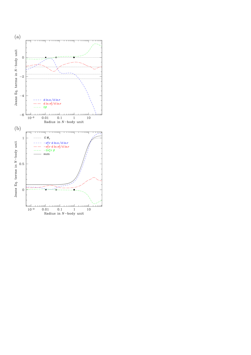
Figure 15: Check of stationary Jeans equation for our “standard” model ($10^{5}$ stars, case a) at $T=10\,Gyrs$ (same model and time as Fig. 7). Panel (a) depicts the logarithmic derivatives of the stellar density $n$ and radial component of the velocity dispersion well as the anisotropy parameter, $2\beta=2-\sigma_{t}^{2}/\sigma_{r}^{2}$. Horizontal lines corresponding to values of $0$, $-1$, $-1.75$ and $-2.23$ are present to guide the eye. In particular, the “Keplerian” velocity profile is ${\rm d}\ln\,\sigma_{r}^{2}/{\rm d}\ln\,r\equiv-1$. The round dot indicates the influence radius, the star the critical radius and the square the “1-star” radius. On panel (b), we plot the three terms of the right side of the stationary Jeans equation and check that their sum is (nearly) equal to the left side term, i.e. $GM_{\rm r}$.

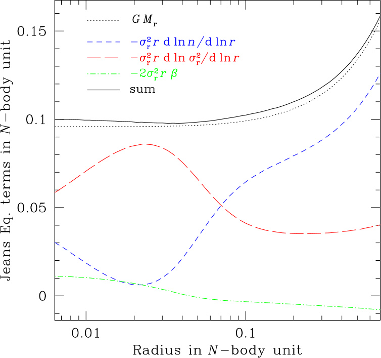
Figure 16: Blow-up of panel (b) of Fig. 15 for the region between the 1-star and the influence radius.

In the region dominated by the central BH, one may expect a “Keplerian” profile for the velocity dispersion, $\sigma\propto r^{-1/2}$. However, in Sec. 4, we have seen that in our standard model ($10^{5}$ stars, case a this relation does not really apply where expected, i.e. between the “1-star” and the influence radius. Here we show that the spherical Jeans equation for a system in dynamical equilibrium is nevertheless obeyed.

In spherical symmetry the assumption of dynamical equilibrium (or stationarity) amounts to $u=\left<v_{\rm r}\right>\equiv 0$. We note that the gaseous model can cope with $u\neq 0$. On the other hand, for a system whose evolution is driven by relaxation, one expects $\sigma_{\rm r,t}\gg u$. The Jeans equation then reads (Binney & Tremaine 1987, Eq. 4-55)

$$GM_{\rm r}=-r\sigma_{\rm r}^{2}\left(\frac{{\rm d}\ln n}{{\rm d}\ln r}+\frac{{\rm d}\ln\sigma_{\rm r}^{2}}{{\rm d}\ln r}+2\beta\right).$$ (71)

$M_{\rm r}$ is the mass enclosed by the radius $r$, $n$ the number density of stars and $2\beta=2-\sigma_{t}^{2}/\sigma_{r}^{2}$ is the anisotropy parameter; other quantities have been defined previously. One sees easily that if $M_{\rm r}\equiv{\cal M}_{\rm bh}$ and the first and third term in the brackets are both constant, $\sigma\propto r^{-1/2}$ at small $r$. But, as figures 15 and 16 demonstrate, none of these assumptions exactly applies in the range of radius under consideration. Consequently, we do not get a clean Keplerian velocity profile although (or because) Eq. 71 is satisfied. Finally, we mention that our models with $10^{6}$ and $10^{7}$ stars (and same initial size) exhibit a Keplerian velocity cusp outside the 1-star radius, during their post-collapse evolution. This is partly due to the relatively more massive black hole (larger influence radius) and partly to the much smaller 1-star radius.

Appendix C MBH wandering in a cuspy cluster.

Here we present a simple estimate of the wandering radius $R_{\rm wan}$ of a MBH embeded in a stellar cluster whose density posseses a power-law cusp in the inner regions. We assume that, were it not for the effect of the MBH itself, the stellar cluster would be described by an eta-model (Dehnen, 1993; Tremaine et al., 1994) with enclosed stellar mass

$${\cal M}_{\ast}(r)={\cal M}_{\rm cl}\left(\frac{r/a}{1+r/a}\right)^{\eta},$$ (72)

where ${\cal M}_{\rm cl}$ is the total mass in stars and $a$ the break radius. For $r\ll a$, the density is $\rho\propto r^{-\alpha}$ with $\alpha=3-\eta$. Inside $R_{\rm wan}$, the MBH strongly perturbates stellar orbits and we suppose the density is rendered more or less constant. Hence, the potential felt by the MBH is approximately harmonic,

$$\Phi(r)=\Phi_{0}+\frac{1}{2}\omega^{2}r^{2}\ \ \mbox{, with}\ \omega^{2}=\frac{G{\cal M}_{\ast}(R_{\rm wan})}{R_{\rm wan}^{3}}.$$ (73)

For a harmonic oscillator, the RMS amplitude of the oscillations in velocity and space are linked to each other,

$$V_{\rm RMS}^{2}=\omega^{2}R_{\rm RMS}^{2}\approx\omega R_{\rm wan}^{2}=\frac{G{\cal M}_{\ast}(R_{\rm wan})}{R_{\rm wan}}.$$ (74)

Dorband et al. (2003) have verified with $N$-body simulations that equipartition of kinetic energy between the MBH and the stars is established, at least in the case of $\eta=1.5$. Namely,

$${\cal M}_{\rm bh}V_{\rm RMS}^{2}\simeq m_{\ast}\sigma^{2},$$ (75)

where $\sigma$ is the stellar velocity dispersion at $r=a$. For $\eta=1.5$ (Tremaine et al., 1994),

$$\sigma^{2}\simeq 0.1\frac{G{\cal M}_{\rm cl}}{a}.$$ (76)

Finally, assuming $R_{\rm wan}\ll a$ and, hence, ${\cal M}_{\ast}(R_{\rm wan})\simeq{\cal M}_{\rm cl}\left(R_{\rm wan}/a\right)^{\eta}$ and combining equations 74, 75 and 76, we obtain

$$R_{\rm wan}\approx 0.01a\left(\frac{m_{\ast}}{{\cal M}_{\rm bh}}\right)^{2}\ \ \mbox{for}\ \eta=1.5$$ (77)

and

$$R_{\rm wan}\propto a\left(\frac{m_{\ast}}{{\cal M}_{\rm bh}}\right)^{1/(\eta-1)}$$ (78)

for general eta-models.

Appendix D Projected velocity dispersions

For the Figures 10 and 9 we have integrated the density along the z-axis for the projection,

$$\Sigma(r)=\int_{z=0}^{z=R_{\rm max}}\rho(\sqrt{r^{2}+z^{2}})\,dz={}$$ (79)

$${}2\int_{r}^{z={R_{\rm max}}}\rho(R)\frac{R}{\sqrt{R^{2}-r^{2}}}\,dR$$

If one observes the cluster along the z-axis, the contributions to the projected velocity dispersions are as indicated in Fig. 17. We have that $R=\sqrt{r^{2}+z^{2}}$ and $\sigma_{\theta}=\sigma_{\phi}=\sigma_{\rm t}$, where the subscript t stands for tangential. We can reckon that

$$\sigma^{2}_{\rm z}=\sigma^{2}_{\rm R}\,\cos^{2}\theta+\tilde{\sigma}^{2}_{\rm t}\sin^{2}\theta$$

$$\sigma^{2}_{\rm r}=\sigma^{2}_{\rm R}\,\sin^{2}\theta+\tilde{\sigma}^{2}_{\rm t}\cos^{2}\theta,$$ (80)

where we have defined $\tilde{\sigma}^{2}_{\rm t}\equiv\sigma^{2}_{\rm t}/2$, to be consistent with the notation used until now.

Figure 17: Different contributions to the projected velocity dispersions. The semi-major axis of the ellipsoid perpendicular to the page corresponds to $\sigma_{\rm t}=\sigma_{\phi}$.

In Fig. 17 we can see that $\sigma_{\rm z}$ contributes to $\sigma_{\rm LOS}$, $\sigma_{\rm r}$ to $\sigma_{\rm pm,r}$ and $\tilde{\sigma}_{\rm t}^{2}$ to $\sigma_{\rm pm,t}$.

Thus, we obtain the projected velocity dispersions,

$$\sigma^{2}_{\rm LOS}(r)=\frac{2}{\Sigma(R)}\int^{R_{\rm max}}_{z=0}(\sigma^{2}_{\rm R}(R)\cos^{2}\theta+\tilde{\sigma}^{2}_{\rm t}(R)\sin^{2}\theta)\rho(R)\,dz={}$$

$${}\frac{2}{\Sigma(R)}\int^{R_{\rm max}}_{z=0}(\frac{z^{2}}{R^{2}}(\sigma^{2}_{\rm R}(R)-\tilde{\sigma}^{2}_{\rm t}(R))+\tilde{\sigma}^{2}_{\rm t}(R))\rho(R)\,dz$$

$$\sigma^{2}_{\rm pm,r}(r)=\frac{2}{\Sigma(R)}\int^{R_{\rm max}}_{z=0}(\sigma^{2}_{\rm R}(R)\sin^{2}\theta+\tilde{\sigma}^{2}_{\rm t}(R)\cos^{2}\theta)\rho(R)\,dz={}$$

$${}\frac{2}{\Sigma(R)}\int^{R_{\rm max}}_{z=0}(\frac{z^{2}}{R^{2}}(\tilde{\sigma}^{2}_{\rm t}(R)-{\sigma}^{2}_{\rm R}(R))+{\sigma}^{2}_{\rm R}(R))\rho(R)\,dz$$

$$\sigma^{2}_{\rm pm,r}(r)=\frac{2}{\Sigma(R)}\int^{R_{\rm max}}_{z=0}\tilde{\sigma}^{2}_{\rm t}(R)\rho(R)\,dz,$$ (81)

since $\sin^{2}\theta=r^{2}/R^{2}=1-\cos^{2}\theta$ and $\cos^{2}\theta=z^{2}/R^{2}$.

References

- Aarseth (1999a) Aarseth S. J., 1999a, PASP, 111, 1333
- Aarseth (1999b) —, 1999b, Celestial Mechanics and Dynamical Astronomy, 73, 127
- Amaro-Seoane & Spurzem (2001) Amaro-Seoane P., Spurzem R., 2001, MNRAS, 327, 995
- Bahcall & Wolf (1976) Bahcall J. N., Wolf R. A., 1976, ApJ, 209, 214
- Baumgardt et al. (2003a) Baumgardt H., Hut P., Makino J., McMillan S., Portegies Zwart S., 2003a, ApJ Lett., 582, L21
- Baumgardt et al. (2003b) Baumgardt H., Makino J., Hut P., McMillan S., Portegies Zwart S., 2003b, ApJ Lett., 589, L25
- Bettwieser (1983) Bettwieser E., 1983, MNRAS, 203, 811
- Bettwieser & Spurzem (1986) Bettwieser E., Spurzem R., 1986, 161, 102
- Bettwieser & Sugimoto (1984) Bettwieser E., Sugimoto D., 1984, MNRAS, 208, 493
- Bettwieser & Sugimoto (1985) —, 1985, MNRAS, 212, 189
- Binney & Tremaine (1987) Binney J., Tremaine S., 1987, Galactic Dynamics. Princeton University Press
- Chatterjee et al. (2002) Chatterjee P., Hernquist L., Loeb A., 2002, ApJ, 572, 371
- Cohn & Kulsrud (1978) Cohn H., Kulsrud R. M., 1978, ApJ, 226, 1087
- da Costa (1981) da Costa L. N., 1981, 195, 869
- David et al. (1987a) David L. P., Durisen R. H., Cohn H. N., 1987a, ApJ, 313, 556
- David et al. (1987b) —, 1987b, ApJ, 316, 505
- Dehnen (1993) Dehnen W., 1993, MNRAS, 265, 250
- Deiters & Spurzem (2001) Deiters S., Spurzem R., 2001, in ASP Conf. Ser. 228: Dynamics of Star Clusters and the Milky Way, p. 416
- Dokuchaev & Ozernoi (1977) Dokuchaev V. I., Ozernoi L. M., 1977, Sov. Astron. Lett., 3, 112
- Dorband et al. (2003) Dorband E. N., Hemsendorf M., Merritt D., 2003, Journal of Computational Physics, 185, 484
- Duncan & Shapiro (1982) Duncan M. J., Shapiro S. L., 1982, ApJ, 253, 921
- Ebisuzaki et al. (2001) Ebisuzaki T., Makino J., Tsuru T. G., Funato Y., Portegies Zwart S., Hut P., McMillan S., Matsushita S., Matsumoto H., Kawabe R., 2001, ApJ Lett., 562, L19
- Ferrarese et al. (2001) Ferrarese L., Pogge R. W., Peterson B. M., Merritt D., Wandel A., Joseph C. L., 2001, ApJ Lett., 555, 79
- Frank & Rees (1976) Frank J., Rees M. J., 1976, MNRAS, 176, 633
- Fregeau et al. (2003) Fregeau J. M., Gürkan M. A., Joshi K. J., Rasio F. A., 2003, 593, 772
- Freitag (2003a) Freitag M., 2003a, Captures of stars by a massive black hole: Investigations in numerical stellar dynamics. to appear in the proceedings of “The Astrophysics of Gravitational Wave Sources”, astro-ph/0306064
- Freitag (2003b) —, 2003b, ApJ Lett., 583, 21
- Freitag & Benz (2001) Freitag M., Benz W., 2001, A&A, 375, 711
- Freitag & Benz (2002) —, 2002, A&A, 394, 345
- Freitag & Benz (2004) —, 2004, A comprehensive set of simulations of high-velocity collisions between main sequence stars. submitted to MNRAS, astro-ph/0403621
- Gürkan et al. (2004) Gürkan M. A., Freitag M., Rasio F. A., 2004, ApJ
- Gebhardt et al. (2001) Gebhardt K., Lauer T. R., Kormendy J., Pinkney J., Bower G., Green R., Gull T., Hutchings J. B., Kaiser M. E., Nelson C. H., Richstone D., Weistrop D., 2001, AJ, 122, 2469
- Gebhardt et al. (2002) Gebhardt K., Rich R. M., Ho L. C., 2002, ApJ Lett., 578, 41
- Gerssen et al. (2002) Gerssen J., van der Marel R. P., Gebhardt K., Guhathakurta P., Peterson R. C., Pryor C., 2002, AJ, 124, 3270
- Gerssen et al. (2003) —, 2003, AJ, 125, 376
- Ghez et al. (2003) Ghez A. M., Duchêne G., Matthews K., Hornstein S. D., Tanner A., Larkin J., Morris M., Becklin E. E., Salim S., Kremenek T., Thompson D., Soifer B. T., Neugebauer G., McLean I., 2003, ApJ Lett., 586, L127
- Giersz (1998) Giersz M., 1998, MNRAS, 298, 1239
- Giersz & Heggie (1994) Giersz M., Heggie D. C., 1994, 270, 298
- Giersz & Spurzem (1994) Giersz M., Spurzem R., 1994, MNRAS, 269, 241
- Giersz & Spurzem (2000) —, 2000, MNRAS, 317, 581
- Giersz & Spurzem (2003) —, 2003, MNRAS, 343, 781
- Goodman (1984) Goodman J., 1984, ApJ, 280, 298
- Gurevich (1964) Gurevich A., 1964, Geomag. Aeronom., 4, 247
- Hénon (1965) Hénon M., 1965, Annales d’Astrophysique, 28, 62
- Hachisu et al. (1978) Hachisu I., Nakada Y., Nomoto K., Sugimoto D., 1978, Prog. Theor. Phys. 60, 393
- Heggie (1984) Heggie D. C., 1984, MNRAS, 206, 179
- Heggie & Mathieu (1986) Heggie D. C., Mathieu R. D., 1986, in The Use of Supercomputers in Stellar Dynamics, Hut P., McMillan S. L. W., eds., Springer-Verlag, p. 233
- Heggie & Ramamani (1989) Heggie D. C., Ramamani N., 1989, 237, 757
- Hénon (1971) Hénon M., 1971, Ap&SS, 13, 284
- Henyey et al. (1959) Henyey L. G., Wilets L., Böhm K. H., Lelevier R., Levee R. D., 1959, ApJ, 129, 628
- Herrnstein et al. (1999) Herrnstein J. R., Moran J. M., Greenhill L. J., Diamond P. J., Inoue M., Nakai N., Miyoshi M., Henkel C., Riess A., 1999, Nat, 400, 539
- Hills (1975) Hills J. G., 1975, Nat, 254, 295
- Joshi et al. (2001) Joshi K. J., Nave C. P., Rasio F. A., 2001, ApJ, 550, 691
- Kippenhahn & Weigert (1994) Kippenhahn R., Weigert A., 1994, Stellar Structure and Evolution. Springer-Verlag Berlin Heidelberg
- Kormendy (2003) Kormendy J., 2003, in “Coevolution of Black Holes and Galaxies”, Carnegie Observatories, Pasadena, Ho L., ed., astro-ph/0306353
- Lightman & Shapiro (1977) Lightman A. P., Shapiro S. L., 1977, ApJ, 211, 244
- Lin & Tremaine (1980) Lin D. N. C., Tremaine S., 1980, ApJ, 242, 789
- Louis & Spurzem (1991) Louis P. D., Spurzem R., 1991, MNRAS, 251, 408
- Lynden-Bell (1967) Lynden-Bell D., 1967, MNRAS, 136, 101
- Lynden-Bell (1969) —, 1969, Nat, 223, 690
- Lynden-Bell & Eggleton (1980) Lynden-Bell D., Eggleton P. P., 1980, MNRAS, 191, 483
- Lynden-Bell & Rees (1971) Lynden-Bell D., Rees M. J., 1971, MNRAS, 152, 461
- Magorrian & Tremaine (1999) Magorrian J., Tremaine S., 1999, MNRAS, 309, 447
- Marchant & Shapiro (1979) Marchant A. B., Shapiro S. L., 1979, ApJ, 234, 317
- Marchant & Shapiro (1980) —, 1980, ApJ, 239, 685
- McMillan et al. (1981) McMillan S. L. W., Lightman A. P., Cohn H., 1981, ApJ, 251, 436
- Merritt et al. (2001) Merritt D., Ferrarese L., Joseph C. L., 2001, Science, 293, 1116
- Miller & Colbert (2003) Miller M. C., Colbert E. J. M., 2003, Intermediate-Mass Black Holes. preprint, astro-ph/0308402
- Milosavljević & Merritt (2003) Milosavljević M., Merritt D., 2003, ApJ, 596, 860
- Miralda-Escudé & Gould (2000) Miralda-Escudé J., Gould A., 2000, ApJ, 545, 847
- Miyoshi et al. (1995) Miyoshi M., Moran J., Herrnstein J., Greenhill L., Nakai N., Diamond P., Inoue M., 1995, Nat, 373, 127
- Moran et al. (1999) Moran J. M., Greenhill L. J., Herrnstein J. R., 1999, Journal of Astrophysics and Astronomy, 20, 165
- Morris (1993) Morris M., 1993, ApJ, 408, 496
- Murphy et al. (1991) Murphy B. W., Cohn H. N., Durisen R. H., 1991, ApJ, 370, 60
- Ozernoi & Reinhardt (1978) Ozernoi L. M., Reinhardt M., 1978, A&AS, 59, 171
- Peebles (1972) Peebles P. J. E., 1972, ApJ, 178, 371
- Pfahl & Loeb (2003) Pfahl E., Loeb A., 2003, ArXiv Astrophysics e-prints
- Pinkney et al. (2003) Pinkney J., Gebhardt K., Bender R., Bower G., Dressler A., Faber S. M., Filippenko A. V., Green R., Ho L. C., Kormendy J., Lauer T. R., Magorrian J., Richstone D., Tremaine S., 2003, ApJ, 596, 903
- Portegies Zwart & McMillan (2002) Portegies Zwart S. F., McMillan S. L. W., 2002, ApJ, 576, 899
- Rasio et al. (2003) Rasio F. A., Freitag M., Gürkan M. A., 2003, in “Coevolution of Black Holes and Galaxies”, Carnegie Observatories, Pasadena, Ho L., ed., astro-ph/0304038
- Rees (1984) Rees M. J., 1984, ARA&A, 22, 471
- Rees (1990) —, 1990, Science, 247, 817
- Schödel et al. (2003) Schödel R., Ott T., Genzel R., Eckart A., Mouawad N., Alexander T., 2003, ApJ, 596, 1015
- Shapiro (1977) Shapiro S. L., 1977, ApJ, 217, 281
- Shapiro & Lightman (1976) Shapiro S. L., Lightman A. P., 1976, Nat, 262, 743
- Sigurdsson (2003) Sigurdsson S., 2003, Classical and Quantum Gravity, 20, 45
- Sołtan (1982) Sołtan A., 1982, MNRAS, 200, 115
- Spitzer (1987) Spitzer L., 1987, Dynamical evolution of globular clusters. Princeton University Press
- Spurzem (1991) Spurzem R., 1991, MNRAS, 252, 177
- Spurzem (1992) —, 1992, in Reviews of Modern Astronomy, Vol. 5, pp. 161–173
- Spurzem (1999) —, 1999, Journal of Computational and Applied Mathematics, 109, 407
- Spurzem & Aarseth (1996) Spurzem R., Aarseth S. J., 1996, MNRAS, 282, 19
- Spurzem & Takahashi (1995) Spurzem R., Takahashi K., 1995, MNRAS, 272, 772
- Syer & Ulmer (1999) Syer D., Ulmer A., 1999, MNRAS, 306, 35
- Takahashi (1995) Takahashi K., 1995, PASJ, 47, 561
- Takahashi (1996) —, 1996, PASJ, 48, 691
- Takahashi (1997) —, 1997, PASJ, 49, 547
- Tremaine et al. (1994) Tremaine S., Richstone D. O., Byun Y., Dressler A., Faber S. M., Grillmair C., Kormendy J., Lauer T. R., 1994, AJ, 107, 634
- van der Marel et al. (2002) van der Marel R. P., Gerssen J., Guhathakurta P., Peterson R. C., Gebhardt K., 2002, AJ, 124, 3255
- Yu & Tremaine (2002) Yu Q., Tremaine S., 2002, MNRAS, 335, 965